Modeling Glacier Elevation Change from DEM Time Series

Abstract

In this study, a methodology for glacier elevation reconstruction from Digital Elevation Model (DEM) time series (tDEM) is described for modeling the evolution of glacier elevation and estimating related volume change, with focus on medium-resolution and noisy satellite DEMs. The method is robust with respect to outliers in individual DEM products. Fox Glacier and Franz Josef Glacier in New Zealand are used as test cases based on 31 Advanced Spaceborne Thermal Emission and Reflection Radiometer (ASTER) DEMs and the Shuttle Radar Topography Mission (SRTM) DEM. We obtained a mean surface elevation lowering rate of −0.51 ± 0.02 m·a⁻¹ and −0.09 ± 0.02 m·a⁻¹ between 2000 and 2014 for Fox and Franz Josef Glacier, respectively. The specific volume difference between 2000 and 2014 was estimated as −0.77 ± 0.13 m·a⁻¹ and −0.33 ± 0.06 m·a⁻¹ by our tDEM method. The comparably moderate thinning rates are mainly due to volume gains after 2013 that compensate larger thinning rates earlier in the series. Terminus thickening prevailed between 2002 and 2007.

1. Introduction

Differencing elevation data is a widely used method to document elevation and volume changes of glaciers (e.g., [1,2,3,4,5,6]). Precise estimation of the development of glacier elevation from space is still challenging due to a lack of sufficiently accurate data. Quantifying detailed glacier volume evolution over large areas worldwide, which is only feasible using spaceborne methods, would help to better understand glacier response to weather and climate, and how glacier change affects for instance sea level and river runoff.

Satellite altimetry data provide good accuracy and temporal resolution, which are highly valuable to quantify glacier changes, but are usually sparsely distributed on the ground. For example, the Ice Cloud and land Elevation Satellite (ICESat) acquired precise elevation data between 2003 and 2009 with a repeat cycle of nominally 91 days (in practice 2–3 times a year) [7], and the data have been widely exploited for deriving change in glacier elevation and volume (e.g., [1,2]). The ICESat mission was primarily dedicated for the measurement of polar ice sheets, and its data have very sparse ground coverage in particular in low-latitude regions [1,8], making it difficult to study individual mountain glaciers. Meanwhile, spaceborne radar and optical stereo DEM data provide almost full ground coverage, but suffer often from inferior quality and outliers, and from variable temporal resolutions, or, respectively, from insufficient acquisition frequencies in order to have enough data available under optimal conditions. However, given the fact that, if combined, a large amount of DEM data from various space sensors (e.g., ASTER, SPOT, Pleiades, WorldView, QuickBird and IKONOS satellite stereo; SRTM and TanDEM-X radar interferometry) are available, satellite-derived DEM time series have a high potential in assessing glacier elevation evolution, which is not yet fully exploited. In simple words, time series of a large number of DEMs could be used to overcome the deficiencies of individual DEMs by statistical means.

Previous DEM-differencing methods used mainly the difference of two DEMs (DEM subtraction) to derive elevation change and volume change (e.g., [4,9,10,11]). However, globally available DEM data are often insufficient for analysis of individual glaciers due to their acquisition principles. For example, DEMs from optical stereo suffer from cloud disturbance or lack of visual contrast on the ground and related problems for parallax matching, while radar data (e.g., the SRTM DEM) may contain voids over steep terrain due to the side-looking sensor principle, and radar waves may penetrate into the snow and ice. Recently, robust linear regression in time from multi-temporal DEMs has been explored (e.g., [3,12,13,14]) and gives more robust results when compared to the subtraction of just two DEMs.

However, both DEM subtraction and regression methods cannot cope with variations in glacier elevation change. Glaciers behave not necessarily linearly in elevation. Especially glaciers that have short reaction times (typically maritime glaciers) fluctuate rapidly to adjust to variations in accumulation and ablation [15]. Hence, linear regression may not be sufficient for a number of glaciers, and in general not for longer DEM time series. Methods that assess higher-order elevation variation are thus needed. [16] developed a Surface Elevation Reconstruction And Change Detection (SERAC) method to detect the surface elevation change of the Greenland Ice Sheet based on ICESat data. The method uses polynomial regressions instead of common linear regression, being able to reconstruct variations of elevation change. Recently, these authors have expanded their method to use analytical models by involving more elevation data sources such as DEMs and airborne laser data [17,18]. To our best knowledge, no such attempts have been applied to mountain glaciers and satellite DEM time series alone, likely due to the often poor quality of individual DEM data sets.

In this study, we present a methodology for glacier elevation reconstruction from DEM time series (tDEM), generating a 4-dimensional (4D) DEM which includes time as an additional dimension to the traditional 3-dimensional spatial coordinates. We describe in this paper the framework of our tDEM method, and application examples for two glaciers in New Zealand. We would like to stress that variations and adaptations of our methodology are possible at many stages, and perhaps even reasonable for specific applications. The purpose of this contribution is rather to discuss the general potential and limitations of DEM time-series analyses for estimation of glacier changes. We would also like to stress that the main focus of this contribution lies on the methodology, and not on glaciological aspects, which will only be discussed to the extent necessary in order to put our results into context.

2. Study Area and Data

2.1. Study Area

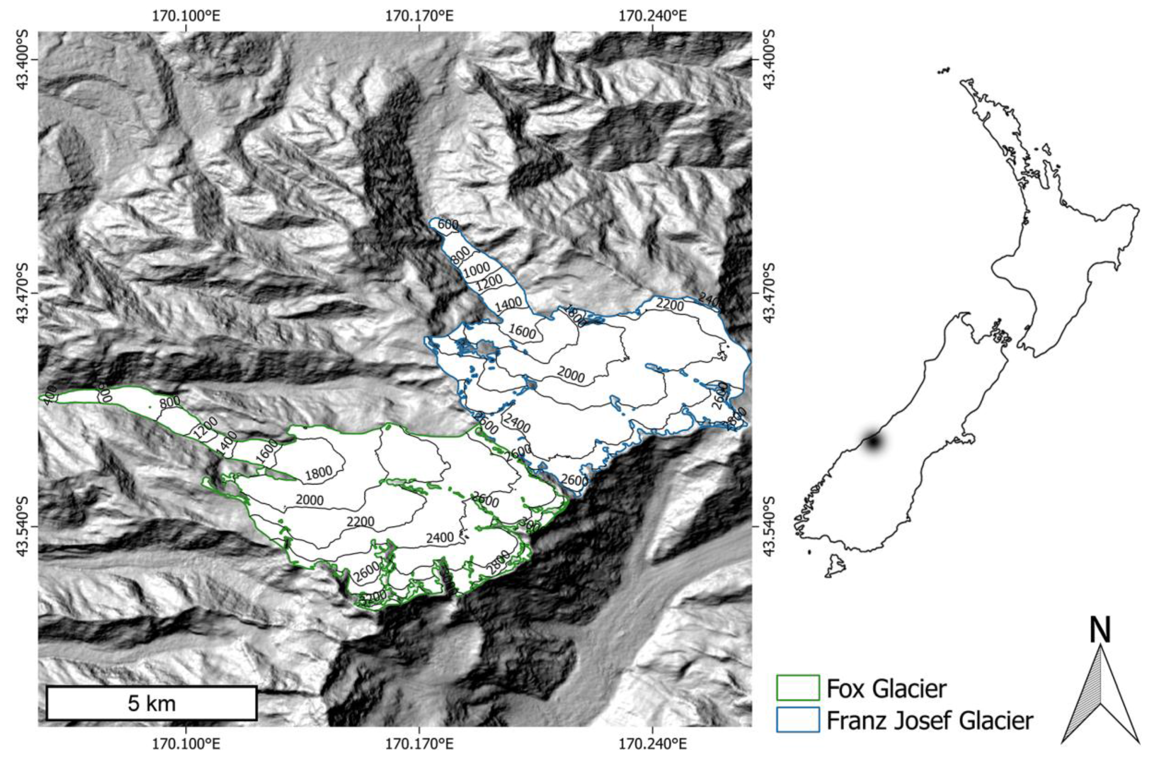
Fox Glacier and Franz Josef Glacier are located on the west side of Mt. Cook in the Southern Alps of New Zealand, with Franz Josef Glacier to the Northeast of Fox Glacier (Figure 1). Both glaciers are well known for their short reaction and response times to variations in accumulation and ablation [19]. Fox Glacier covers an area of ~ 35 km², presently (2014) with elevations ranging from ~ 260 m above sea level (a.s.l.) at terminus to ~ 3500 m a.s.l. at the highest peak. It has a large flat accumulation area, with a steep glacier tongue that feeds ice down into a narrow valley. The Franz Josef Glacier features similar characteristics as Fox Glacier, ranging from elevations of ~350 m a.s.l. to ~2940 m a.s.l. Both glaciers were here chosen as case studies due to their short reaction times and thus potentially non-linear elevation development, and due to the good availability of ASTER stereo data.

Franz Josef and Fox Glaciers are very maritime with assumed precipitation rates of up to 12 m·w.e.a⁻¹ [19,20,21,22]. Ablation at the tongues is substantial at all seasons with a mean summer ablation of ~130 mm·d⁻¹ and a mean winter ablation of ~20 mm·d⁻¹, i.e., several tens of meters as annual sum [23]. The two glaciers are believed to react especially sensitive to temperature variations, with reaction and response times of only around 3–4 and 10–20 years, respectively [22,23,24]. Glacier elevation close to the tongues is able to change by many tens of meters within just a few years, and lateral terminus position by several hundred meters [15,25]. Glacier speeds are up to several m·d⁻¹ and can also change substantially within few years [25]. A phase of pronounced glacier advance from the mid 1980s to around 2000 has been attributed to variations in atmospheric circulation patterns (ENSO) [19,26].

2.2. SRTM DEM

The Shuttle Radar Topography Mission (SRTM) was carried on Space Shuttle Endeavor, and acquired data from 11 to 22 February 2000 between latitudes 60°N and 57°S [27]. The C-band SRTM DEM is available via the U.S. Geological Survey (USGS) at a resolution of 1 arc second (~30 m grid) globally. We use this C-band SRTM DEM as the reference dataset to compare and co-register other DEMs, similar to many other studies (e.g., [14,28]). The vertical accuracy of the SRTM DEM over our study region is estimated as ±10 m at 90% confidence [29].

Here, we use the original SRTM DEM from USGS, rather than any void-filled version, as the filled data over voids tend to be implausible in rugged terrain such as high mountains. However, our tDEM method is by design also able to cope with potentially inconsistent SRTM void fills.

Figure 1. Study area. Shaded relief showing Fox Glacier and Franz Josef Glacier located in the Southern Alps, New Zealand. Glacier extents are from the Randolph Glacier Inventory [30].

Figure 1. Study area. Shaded relief showing Fox Glacier and Franz Josef Glacier located in the Southern Alps, New Zealand. Glacier extents are from the Randolph Glacier Inventory [30].

2.3. ASTER DEM

The Advanced Spaceborne Thermal Emission and Reflection Radiometer (ASTER) is an imaging instrument onboard the Terra satellite [31]. It consists of three separate subsystems, the visible and near infrared (VNIR, 15 m resolution), the shortwave infrared (SWIR, 60 m resolution), and the thermal infrared (TIR, 90 m resolution). The visible and near infrared (VNIR, 15 m resolution) subsystem contains two telescopes, a nadir and a back-looking one, for constructing stereo pairs. These stereo data are used to generate the ASTER standard product AST14DEM, a DEM that is computed by the Land Processes Distributed Active Archive Center (LPDAAC) using the SilcAst software. For good ground conditions the vertical accuracy of ASTER DEMs has been estimated to be on the order of 10 to 20 m, or better if biases are removed [28], with however potential outliers of tens to hundreds of meters, for instance over steep terrain or insufficient visual contrast (Figure 2).

We use the individual AST14DEM products because we are interested in reconstructing a time series of glacier elevation change. Hence, temporally merged DEMs such as the ASTER GDEM are not very suitable for our approach. We selected 31 ASTER DEMs (Table 1) with limited cloud cover and obtained them from LPDAAC.

In order to aid the assessment of effects from seasonal snow cover we also roughly evaluate the percentage snow cover on the two glaciers studied for each DEM date (Table 1; see also figure in Section 3.2.2). Based on visible, near-infrared and short-wave infrared bands of the ASTER images of the according DEM dates we visually estimate the mean snow line elevation and convert it to area percentage using the glaciers hypsometry.

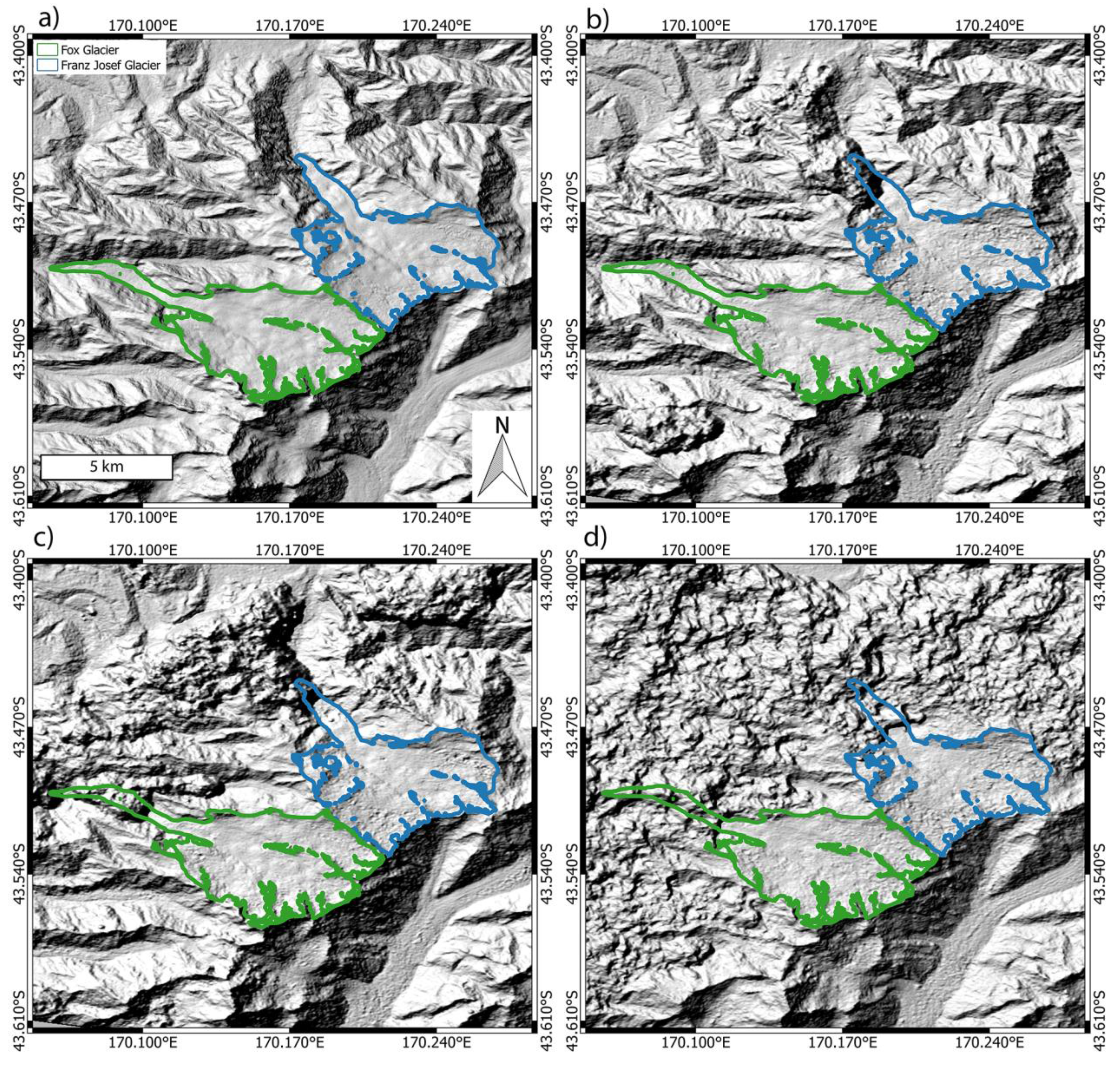
Figure 2. Different typical example ASTER DEMs over the study area. (a) ASTER GDEM2 features smooth terrain without outliers (b) ASTER DEM 2001/04/07 contains noticeable outliers over the glacier tongues, as do (c) ASTER DEM 2001/08/09 and (d) ASTER DEM 2014/02/24. The examples illustrate that any time series analysis has to be particularly robust against elevation outliers.

Figure 2. Different typical example ASTER DEMs over the study area. (a) ASTER GDEM2 features smooth terrain without outliers (b) ASTER DEM 2001/04/07 contains noticeable outliers over the glacier tongues, as do (c) ASTER DEM 2001/08/09 and (d) ASTER DEM 2014/02/24. The examples illustrate that any time series analysis has to be particularly robust against elevation outliers.

2.4. Topographic DEM and Glacier Outlines

A New Zealand national DEM generated based on topographic contours from 1986 aerial photos [32] is in parts incorporated into this study to extent the study time period. The topographic DEM has a ground resolution of 15 m. The vertical accuracy is estimated as ~ 11 m when compared to the SRTM DEM (Table 1). Glacier outlines used are provided by the Randolph Glacier Inventory (RGI 4.0) [30].

Table 1. Summary of Digital Elevation Model (DEM) data and co-registration. σ refers to the original standard deviation (std) of elevation difference (dh) for off-glacier terrain between each DEM and the Shuttle Radar Topography Mission (SRTM) DEM. σ¯ denotes the standard deviation after co-registration. Cloud cover refers to the entire scene, snow cover only to Fox and Franz Josef Glaciers.

Source	Date	Scene ID	Cloud (%)	Horizontal Shift (m)	σ	σ¯	Improvement in std (%)	Snow Cover (%)
Airphoto	1986	–	–	8.6	14.1	11.1	21	–
ASTER	2001/04/07	AST_L1A.003:2007486672	10	18.5	20.9	18.0	14	81
	2001/06/03	AST_L1A.003:2003230186	22	34.1	30.1	20.9	31	88
	2001/07/12	AST_L1A.003:2004198161	11	19.1	20.8	16.7	20	92
	2001/08/29	AST_L1A.003:2004062014	5	12.7	15.8	12.3	22	96
	2002/01/29	AST_L1A.003:2005925463	7	20.7	22.0	12.9	41	64
	2002/02/07	AST_L1A.003:2005981100	25	17.1	26.1	20.0	24	54
	2002/02/14	AST_L1A.003:2013763401	13	13.5	19.2	15.1	21	54
	2002/03/09	AST_L1A.003:2006258979	15	29.2	18.3	14.3	22	92
	2002/12/31	AST_L1A.003:2011854558	12	20.8	22.5	13.8	39	84
	2003/02/24	AST_L1A.003:2011883607	14	17	18.5	17.0	8	90
	2004/02/04	AST_L1A.003:2020707077	54	21.3	30.1	26.9	11	88
	2006/01/24	AST_L1A.003:2032779583	14	12.9	19.8	14.0	30	84
	2006/02/09	AST_L1A.003:2033045873	25	32.6	22.7	17.4	23	64
	2007/12/06	AST_L1A.003:2063467047	12	25.5	23.1	13.0	44	87
	2009/02/17	AST_L1A.003:2070928906	15	37.9	19.2	14.7	24	64
	2010/04/09	AST_L1A.003:2078960682	14	62.4	25.6	17.9	30	53
	2011/12/31	AST_L1A.003:2090572716	7	33.8	21.0	17.3	18	87
	2012/02/26	AST_L1A.003:2091434311	21	16.3	24.3	22.7	7	65
	2012/03/20	AST_L1A.003:2091819125	6	26.4	19.8	15.5	22	63
	2012/04/05	AST_L1A.003:2092063972	13	30.6	21.3	17.0	20	63
	2012/04/21	AST_L1A.003:2092286611	24	20.7	21.4	18.2	15	82
	2012/04/30	AST_L1A.003:2092444675	11	21.8	24.8	22.6	9	91
	2012/06/08	AST_L1A.003:2092964327	31	17.4	23.5	21.3	9	93
	2013/02/19	AST_L1A.003:2123041126	18	30.8	26.0	21.6	17	85
	2013/02/21	AST_L1A.003:2123072945	40	23.1	30.3	26.0	14	88
	2013/06/13	AST_L1A.003:2124729946	23	31	30.6	25.7	16	87
	2014/02/08	AST_L1A.003:2130620243	49	18.7	22.2	17.8	20	85
	2014/02/24	AST_L1A.003:2130823880	60	21.3	22.0	16.4	26	92
	2014/03/26	AST_L1A.003:2131494791	15	38.7	19.2	14.9	22	85
	2014/05/13	AST_L1A.003:2132173961	15	30.9	22.3	18.5	17	88
	2014/05/29	AST_L1A.003:2132389473	17	27.7	20.4	16.7	18	87

Table 1. Summary of Digital Elevation Model (DEM) data and co-registration. σ refers to the original standard deviation (std) of elevation difference (dh) for off-glacier terrain between each DEM and the Shuttle Radar Topography Mission (SRTM) DEM. σ¯ denotes the standard deviation after co-registration. Cloud cover refers to the entire scene, snow cover only to Fox and Franz Josef Glaciers.

Source	Date	Scene ID	Cloud (%)	Horizontal Shift (m)	σ	σ¯	Improvement in std (%)	Snow Cover (%)
Airphoto	1986	–	–	8.6	14.1	11.1	21	–
ASTER	2001/04/07	AST_L1A.003:2007486672	10	18.5	20.9	18.0	14	81
	2001/06/03	AST_L1A.003:2003230186	22	34.1	30.1	20.9	31	88
	2001/07/12	AST_L1A.003:2004198161	11	19.1	20.8	16.7	20	92
	2001/08/29	AST_L1A.003:2004062014	5	12.7	15.8	12.3	22	96
	2002/01/29	AST_L1A.003:2005925463	7	20.7	22.0	12.9	41	64
	2002/02/07	AST_L1A.003:2005981100	25	17.1	26.1	20.0	24	54
	2002/02/14	AST_L1A.003:2013763401	13	13.5	19.2	15.1	21	54
	2002/03/09	AST_L1A.003:2006258979	15	29.2	18.3	14.3	22	92
	2002/12/31	AST_L1A.003:2011854558	12	20.8	22.5	13.8	39	84
	2003/02/24	AST_L1A.003:2011883607	14	17	18.5	17.0	8	90
	2004/02/04	AST_L1A.003:2020707077	54	21.3	30.1	26.9	11	88
	2006/01/24	AST_L1A.003:2032779583	14	12.9	19.8	14.0	30	84
	2006/02/09	AST_L1A.003:2033045873	25	32.6	22.7	17.4	23	64
	2007/12/06	AST_L1A.003:2063467047	12	25.5	23.1	13.0	44	87
	2009/02/17	AST_L1A.003:2070928906	15	37.9	19.2	14.7	24	64
	2010/04/09	AST_L1A.003:2078960682	14	62.4	25.6	17.9	30	53
	2011/12/31	AST_L1A.003:2090572716	7	33.8	21.0	17.3	18	87
	2012/02/26	AST_L1A.003:2091434311	21	16.3	24.3	22.7	7	65
	2012/03/20	AST_L1A.003:2091819125	6	26.4	19.8	15.5	22	63
	2012/04/05	AST_L1A.003:2092063972	13	30.6	21.3	17.0	20	63
	2012/04/21	AST_L1A.003:2092286611	24	20.7	21.4	18.2	15	82
	2012/04/30	AST_L1A.003:2092444675	11	21.8	24.8	22.6	9	91
	2012/06/08	AST_L1A.003:2092964327	31	17.4	23.5	21.3	9	93
	2013/02/19	AST_L1A.003:2123041126	18	30.8	26.0	21.6	17	85
	2013/02/21	AST_L1A.003:2123072945	40	23.1	30.3	26.0	14	88
	2013/06/13	AST_L1A.003:2124729946	23	31	30.6	25.7	16	87
	2014/02/08	AST_L1A.003:2130620243	49	18.7	22.2	17.8	20	85
	2014/02/24	AST_L1A.003:2130823880	60	21.3	22.0	16.4	26	92
	2014/03/26	AST_L1A.003:2131494791	15	38.7	19.2	14.9	22	85
	2014/05/13	AST_L1A.003:2132173961	15	30.9	22.3	18.5	17	88
	2014/05/29	AST_L1A.003:2132389473	17	27.7	20.4	16.7	18	87

3. Method

3.1. DEM Co-Registration

First, we co-register all ASTER DEMs and the topographic DEM to the SRTM DEM by the method proposed by [28], leaving all the DEMs horizontally and vertically aligned properly in order to calculate glacier elevation without major first-order biases. This method corrects potential horizontal shifts and vertical biases based on their relationship with terrain slope and aspect over off-glacier terrain. Removal of vertical biases also reduces the effect of different snow depths during the ASTER DEM acquisition times to the extent to which off-glacier snow depths are representative for on-glacier ones. We found that the relative co-registration accuracies of the ASTER DEMs range from approximately ±13 m to ±27 m for off-glacier terrain and in comparison to the SRTM DEM (Table 1). The worst accuracy belongs to the product with date 2004/02/04, in which a high percentage of cloud coverage led to a poor DEM quality.

3.2. DEM Time Series (tDEM)

3.2.1. Outlier Filtering with Reference Elevations

DEMs from satellite optical stereo, in particular from medium spatial and radiometric resolution images such as ASTER (15 m spatial resolution, 8 bit radiometric resolution), typically contain outliers, for instance caused by clouds and low visual contrast in images, or by image distortions over steep terrain. Filtering such outliers becomes critical for studying glacier surface elevation. Unlike many other studies (e.g., [4,33]) which apply post-processing methods such as thresholds of elevation changes based on their standard deviation to optimize their results, we attempt to eliminate outliers before calculation of elevation changes. Typical statistical outlier detection algorithms take mean values or standard deviation into account. However, in such cases both mean value and standard deviation are already influenced by outliers. Thus, these methods work if the elevation differences are normally distributed [34], but are problematic if only a limited number of samples are available. Our tDEM method solves this problem by dividing DEM pixels into two categories; one where reference data are available, and the other where there are no or insufficient reference data such as pixels in the voids of the SRTM DEM. As the SRTM DEM is regarded as the reference DEM in our study, only pixels that fall over SRTM voids will have no reference data.

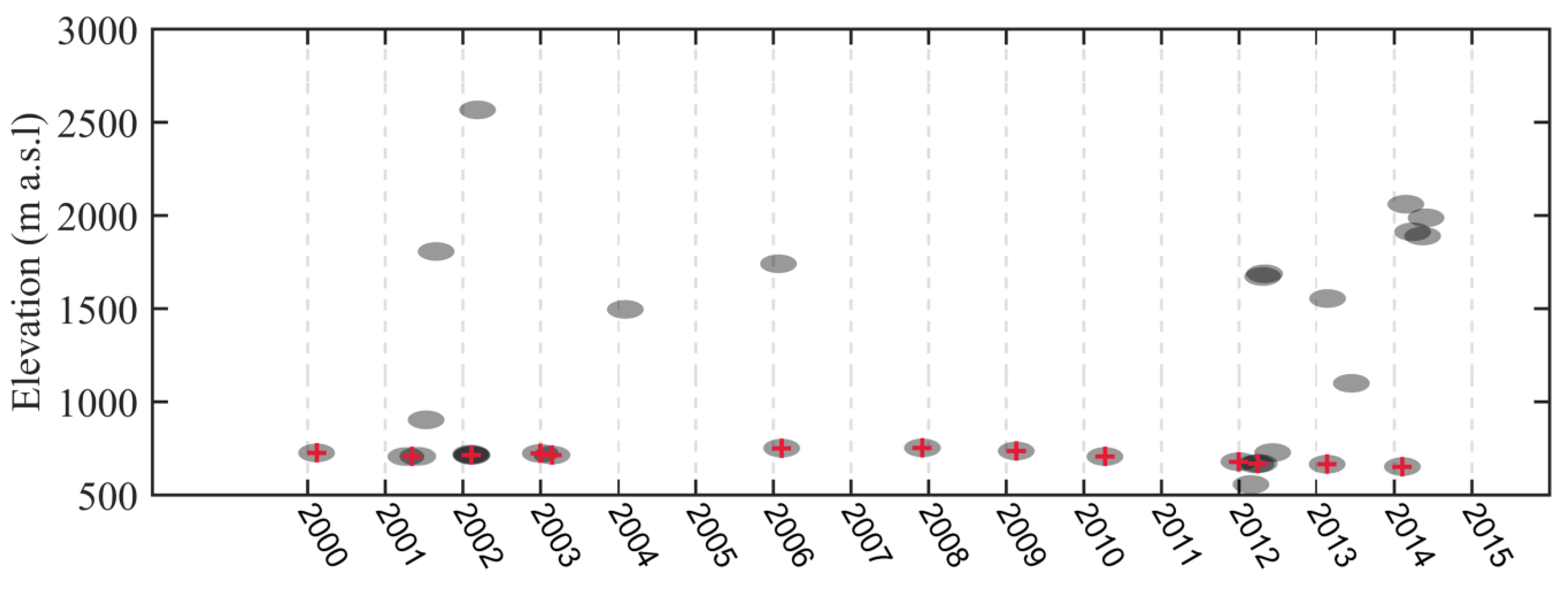
For pixels with sufficient reference data available, a method that involves upper and lower extreme elevation changes is applied. We assume that a maximum glacier elevation thickening rate of +10 m·a⁻¹ and a maximum thinning rate of −30 m·a⁻¹ from the reference data (the SRTM DEM in our study) can happen within the study time period. We set such non-symmetric limitations based on the reason that thickening should not exceed the maximum precipitation, unless glacier surging or other dynamic instabilities happen. Therefore, we believe that +10 m·a⁻¹ of thickening is reasonable for cutting off extreme high elevations. A value of −30 m·a⁻¹ is sufficient enough to capture rapid thinning, and is similar to the ablation at the glacier termini. In fact, changing the upper limit of +10 m·a⁻¹ to +30 m·a⁻¹ will slightly lower the estimated specific volume loss rate over 2000–2014 from −0.77 ± 0.13 m·a⁻¹ to −0.71 ± 0.12 m·a⁻¹ (Fox Glacier ) and −0.33 ± 0.06 m·a⁻¹ to −0.18 ± 0.04 m·a⁻¹ (Franz Josef Glacier). However, allowing +30 m·a⁻¹ thickening would total to 420 m thickening over the 14 years of study period, which is not plausible and would likely capture low clouds. It is, however, clear, that sensitivity tests with different cut-off ranges seem in general advisable to avoid related biases. In our case we chose to keep +10 m·a⁻¹ as upper bound. In addition, we would like to stress that such thresholds are applied to individual pixels for excluding outliers, and before calculating elevation and volume change, rather than to the results of calculated elevation change rate (dh/dt). The simple method works well, as illustrated in Figure 3.

Figure 3. An example of outlier filtering. Data corresponding to point 1 in figure in Section 3.2.3. Gray dots are original DEM elevations. Several extreme high values are likely due to clouds or parallax mismatches. Red crosses are filtered data and grouped by every half year. Years on the horizontal axis refer to 1 January of each year.

Figure 3. An example of outlier filtering. Data corresponding to point 1 in figure in Section 3.2.3. Gray dots are original DEM elevations. Several extreme high values are likely due to clouds or parallax mismatches. Red crosses are filtered data and grouped by every half year. Years on the horizontal axis refer to 1 January of each year.

3.2.2. Outlier Filtering without Reference Elevations

For pixels that have no reference data, the RANSAC (RANdom SAmple Consensus) algorithm is employed. RANSAC is an algorithm proposed originally by [35], for smoothing data that contain a certain percentage of outliers. RANSAC randomly selects a minimum amount of necessary data to define an initial model, incorporating as much valid data into the model as possible. This is the opposite approach to those algorithms that take as much as possible data into consideration to achieve an initial model, and then try to diminish the impact of outliers. The mechanism of RANSAC is summarized as follows:

• A pre-defined model is needed to smooth the data. This model can be any mathematical functions such as a line, or a plane.
• Randomly select the amount of data that is minimally required for determining the parameters for the model (e.g., two points for a line, three points for a plane).
• Give a criterion evaluating if a data point belongs to the defined model.
• Find all the data that belong to the model.
• Repeat steps i–iv, until a best model is found, which is defined as the one that has the maximum amount of data included (in step iv).

In this study, a linear model is configured to filter the elevation data pixel-wise:

$$h=a \cdot t+b$$

(1)

where t refers to time, h refers to elevation. The linear model needs two points to determine the coefficients a and b. An allowance criterion of ±100 m is defined, as it is appropriate to remove cloud effects in ASTER DEMs. At the same time, 100 m seems reasonable to include even large and non-linear glacier thickness changes. Once the model is determined, all data that have a vertical difference from the model value smaller than 100 m are considered as valid data. This is done iteratively to find the best model. The iteration time needed to achieve a good result is defined as

$$P=1-{(1-{(1-\epsilon )}^m)}^M$$

(2)

where P is the possibility to achieve a good model and the corresponding dataset; m is the minimum amount of data required for determining the model; ε is the estimated percentage of error in data; M is the minimum number of iterations in order to achieve a confident possibility P. For example, in our study, 31 ASTER DEMs are involved in the calculation for each pixel. The error percentage is set to 30%. For one pixel, ε = 0.3, m = 2, the minimum iteration time M is 18 in order to achieve a good dataset with a 99.999% confidence possibility, according to Equation 2. The 18 iterations will result in 18 dataset selections with corresponding models. The model that includes most points in time will be identified as the best model, and its corresponding dataset is the final filtered dataset for this pixel. All DEM pixels without reference data (here the original SRTM DEM) available are treated with the same procedure. Consequently, outliers are filtered out for each pixel.

We have employed the RANSAC outlier filtering method for pixels that have no reference data, along with the extreme elevation change threshold method for pixels that have reference data. Such strategy aims at excluding outliers before calculating the elevation change rate dh/dt and volume change. We chose to apply the threshold method preferentially wherever possible, because reference data are plausible and can be viewed as a good selection criterion. However, applying the RANSAC method over all pixels, including those with valid reference data, will only slightly change the results from −0.33 ± 0.06 m·a⁻¹ to −0.31 ± 0.06 m·a⁻¹ for Franz Josef Glacier, while no significant change is found for Fox Glacier. Our combined strategy tends to give optimal results because it takes advantage of the large proportion of available reference data, but our analyses suggest that our tDEM methods works equally fine with RANSAC only, i.e., without having to select one DEM as reference DEM for outlier detection.

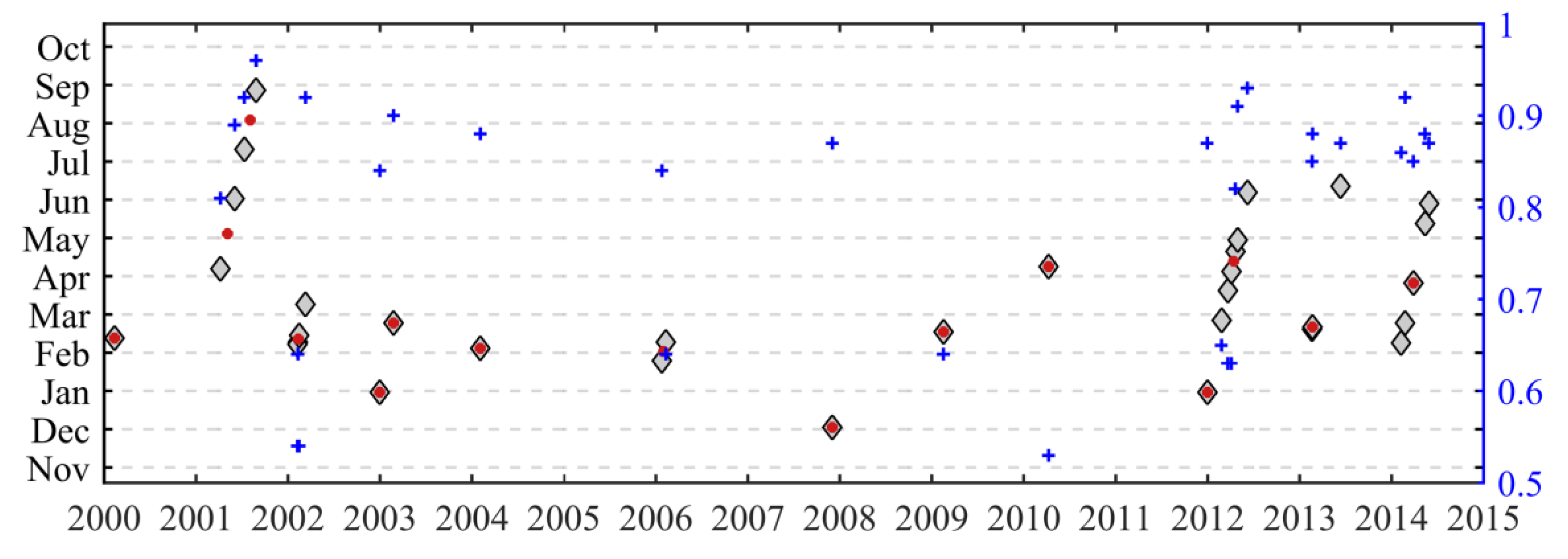
Finally, we evenly distribute the data over time by using the median elevation and acquisition time for each DEM pixel if multiple data are available between any two consecutive half calendar years. For example, six DEMs are available between January and June 2012 (Figure 4) in our study, whereas only one data set (the median) will be used further. This processing is to uniformly distribute data over the study period and to avoid the impacts of temporally clustered DEMs, such as from seasonal effects (e.g., [36]).

Figure 4. Fraction of year of the acquisition dates (displayed as month, left axis) for each DEM (gray diamonds), and grouped by every half calendar year using median values (red dots). Note that in our procedure this grouping is actually done pixel-wise and only average values are indicated as red dots. The right axis (blue) indicates the average fraction of snow cover (between 0.5, 50%, to 1, 100%) for the two glaciers and each acquisition date (blue crosses). Years on the horizontal axis refer to 1 January of each year.

Figure 4. Fraction of year of the acquisition dates (displayed as month, left axis) for each DEM (gray diamonds), and grouped by every half calendar year using median values (red dots). Note that in our procedure this grouping is actually done pixel-wise and only average values are indicated as red dots. The right axis (blue) indicates the average fraction of snow cover (between 0.5, 50%, to 1, 100%) for the two glaciers and each acquisition date (blue crosses). Years on the horizontal axis refer to 1 January of each year.

3.2.3. Modeling Scheme

We developed a “polynomial – spline” modeling scheme within our tDEM method for the elevation variation at each individual pixel. First, a simple weighted linear regression is performed pixel-wise to the filtered data to fit the trend of elevation change. Each elevation is weighted inversely by its accuracy. If the coefficient (slope) of the regression line passes the Student's t-test (95%), a corresponding linear model is assigned to the pixel. Otherwise, the pixel data will in a second step be fitted using a weighted quadratic regression. Similarly, if the coefficient of the highest order turns out to be significant, the pixel's elevation development is described by a weighted quadratic model. If not, the same procedure is repeated in a third step with a cubic model. If a pixel cannot be assigned a linear, quadratic or cubic model, the robust spline fit [37] is performed in a forth step. The spline fit is also known as Piecewise Linear Approximation [38], which in our method divides data equally into two groups, and employs a robust cubic regression to each group. In this way, two cubic curves connected together are sufficient enough to model a polytrophic elevation evolution. The process is done pixel-wise so that a 4-dimensional (4D) model can be finalized by integrating pixels over the whole glacier. The 4D model contains the 3D coordinates of the glacier and adds time as an additional dimension in the form of linear, quadratic, cubic or spline model parameters.

Another advantage of our tDEM method is that it is able to calculate dh/dt at any time by simply computing the first derivative of the modelled curves. We select the mean annual dh/dt over the study time period as the final dh/dt value for each DEM pixel. [16] used the same method when calculating dh/dt of the Greenland ice sheet from ICESat data, whereas other studies fit a linear trend to estimate the overall dh/dt.

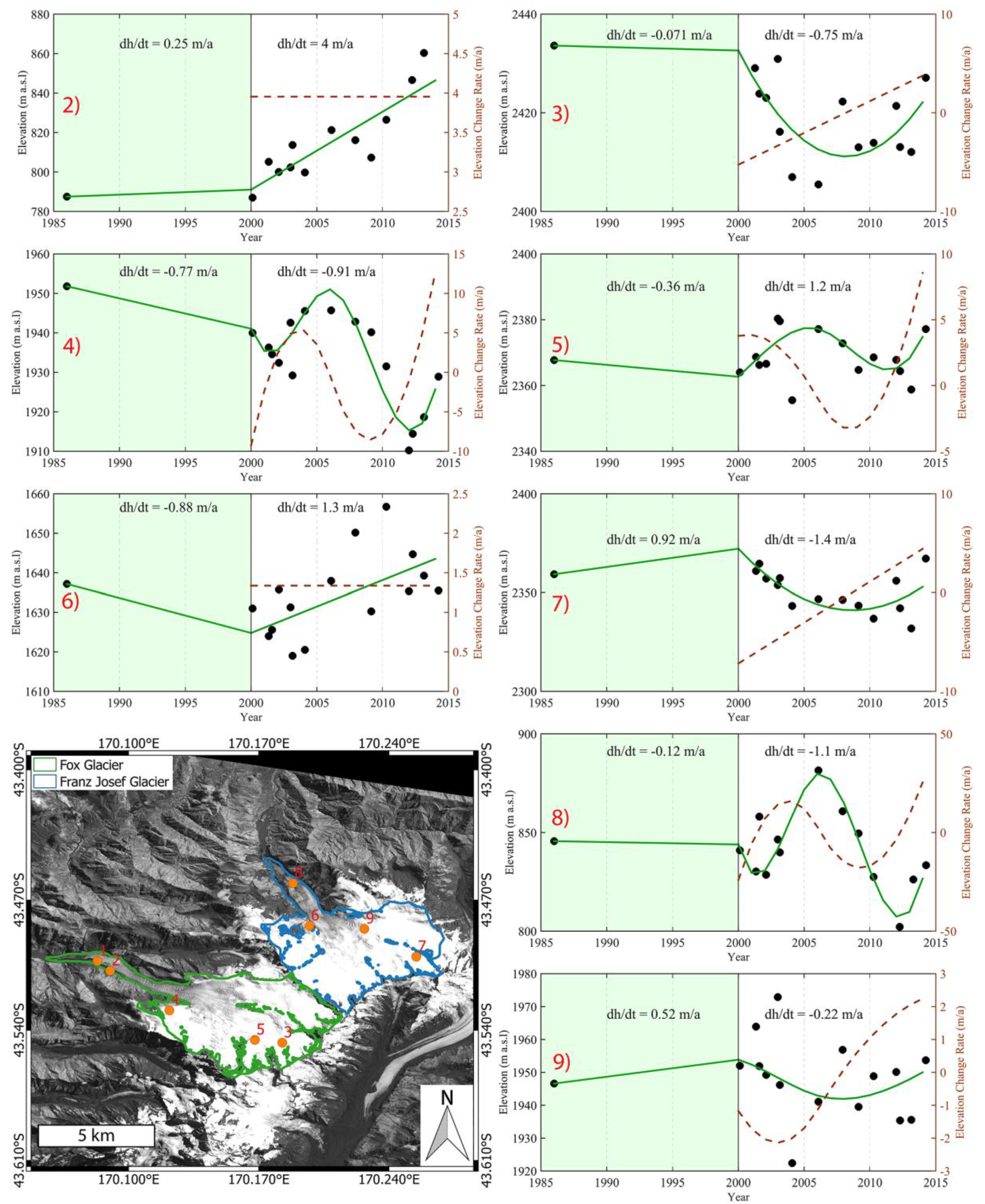
Figure 5 demonstrates some examples of this modeling scheme. Among the numbered pixels of elevation developments, pixel 2 and 6 are automatically assigned a linear model, pixel 3 and 7 are described by a quadratic model, and others are modelled by a spline. In fact, the majority of pixels (96%) are assigned spline models, and no pixel has been assigned a cubic model, indicating that the glaciers investigated are changing their elevation in a complex, and certainly not simply linear way. This is not unexpected for the maritime type of the coastal glaciers in the Southern Alps of New Zealand.

Figure 5. Elevation and elevation change (dh/dt) for selected pixels over the study region. The numbered circles indicate the location of corresponding panels. All datasets passed the outlier filtering method introduced in Section 3.2.1. The left most point of each graph represents the 1986 airphoto DEM, with the second one being the SRTM DEM. The remaining points are from ASTER DEMs. The left part with light green background in each graph represents elevation change between 1986 and 2000, modelled by a simple linear regression (dark green line). The right part is modelled using tDEM (dark green line). Dashed orange lines show the corresponding dh/dt. For point 1 see Figure 3. Years on the horizontal axis refer to 1 January of each year.

Figure 5. Elevation and elevation change (dh/dt) for selected pixels over the study region. The numbered circles indicate the location of corresponding panels. All datasets passed the outlier filtering method introduced in Section 3.2.1. The left most point of each graph represents the 1986 airphoto DEM, with the second one being the SRTM DEM. The remaining points are from ASTER DEMs. The left part with light green background in each graph represents elevation change between 1986 and 2000, modelled by a simple linear regression (dark green line). The right part is modelled using tDEM (dark green line). Dashed orange lines show the corresponding dh/dt. For point 1 see Figure 3. Years on the horizontal axis refer to 1 January of each year.

We want to stress that missing boundary data in regression could cause problems when fitting curves over data boundaries. In our study, SRTM voids caused a lack of data for the year 2000, the early boundary. We also notice that some areas have voids at the late boundary (around the year 2014) due to cloud coverage or pixel mismatches in DEMs after January 2014, so that affected elevation values have been removed through outlier filtering. Since we reconstruct DEMs annually between 2000 and 2014, such points need be treated specially. First, we exclude corresponding data for the year 2000, 2001 and 2014 for which data are implausible due to curve fitting across temporal data boundaries. We then apply the Delta Surface Fill Method (DSF), a technique pioneered by [39], which uses inverse distance weighted interpolation to fill these data.

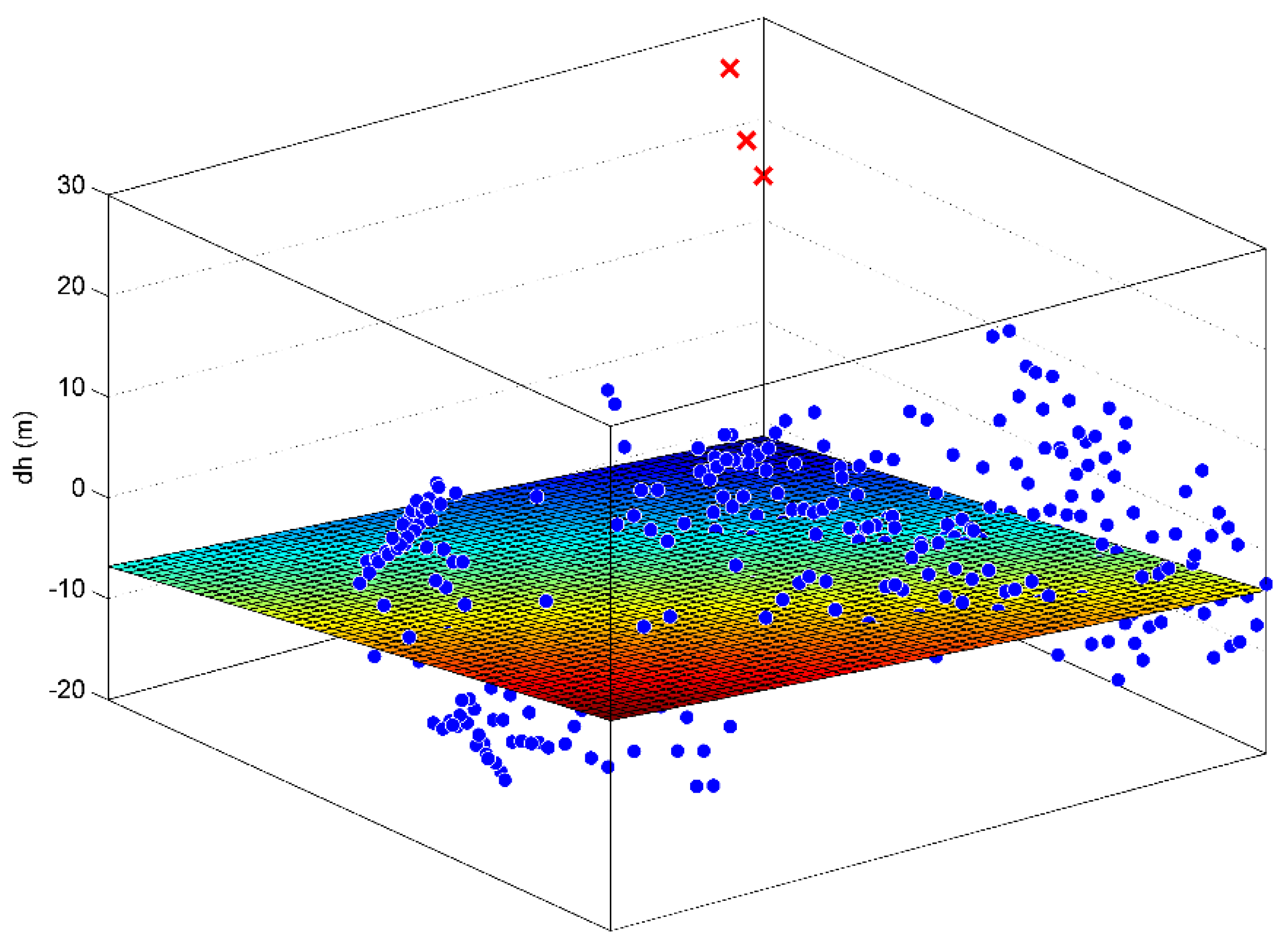
Afterwards, the tDEM method detects blunders that may be caused by wrong curve fitting in reconstructed DEMs. When calculating annual elevation changes, certain regions (e.g., 1 km × 1 km) on the glacier surface are expected to have similar changes. We approximate the local glacier region by a simple plane (Equation 3). The unknown parameters are solved by least squares. Then the residuals larger than three times the standard error are identified as blunders, and thus excluded from the next iteration (Figure 6). The detection stops when no blunders are identified. Finally, all identified blunders are substituted by values calculated from the fitted plane while the remaining accepted elevation changes are used as they are.

$$A \cdot x+B \cdot y+C \cdot dh+D=0$$

(3)

Unlike other studies, which convert elevation change to volume change rate (dv/dt) by multiplying dh/dt by the corresponding glacier area, our tDEM method reconstructs the time series of glacier elevations for each possible pixel. In this way, the volume change (dv) is simply calculated by subtracting the reconstructed DEMs between selected times.

Figure 6. Example of fitted plane through elevation changes over a region. Red crosses stand for the points that had been identified as blunders by previous iterations, and thus excluded from current fitting.

Figure 6. Example of fitted plane through elevation changes over a region. Red crosses stand for the points that had been identified as blunders by previous iterations, and thus excluded from current fitting.

3.3. Uncertainty Assessment

The sources of uncertainties in our method include uncertainty in individual pixel elevations in each DEM product, penetration of C-band radar and the glacier area change. We have used the SRTM DEM as the reference DEM and co-registered all other DEMs to it for off-glacier terrain. The vertical accuracy of the SRTM DEM over the New Zealand region (${\mathrm{\epsilon }}_{\mathrm{s}}$) is estimated as approximately ±10 m [30]. Table 1 summarizes the relative standard error of each DEM (${\mathrm{\sigma }}_{\mathrm{i}}$) compared to the SRTM DEM. That way we can estimate an absolute accuracy of each DEM (${\mathrm{\epsilon }}_{\mathrm{i}}$) following error propagation of Equation 4, where ${\mathrm{\epsilon }}_{\mathrm{s}}$ is the vertical accuracy of the SRTM DEM.

$${\mathrm{\epsilon }}_{\mathrm{i}}=\sqrt{{{\mathrm{\epsilon }}_{\mathrm{s}}}^2+{{\mathrm{\sigma }}_{\mathrm{i}}}^2}$$

(4)

Following, we consider the uncertainty associated with the estimated dh/dt (${\mathrm{\sigma }}_{\mathrm{t}}$). When performing a linear regression, the standard error of estimated parameters can be easily retrieved from the model covariance matrix [16], which takes the accuracy of elevations (ε) into account. In our tDEM method, various models are involved, making the uncertainty estimation complicated. We thus estimate the uncertainty of dh/dt by fitting a linear trend, even when a higher-order model is used to model dh/dt in our method for a specific pixel. In linear regression, the standard error of the estimated slope directly provides the uncertainty of our dh/dt. This simple and common approach is also convenient for comparing our results with other studies. Then the quadratic mean (reduced by effective number of observations; see below) of all the ${\mathrm{\sigma }}_{\mathrm{t}}$ is calculated as the uncertainty of the averaged dh/dt. We obtain a ${\mathrm{\sigma }}_{\mathrm{t}}$ of ±0.02 m·a⁻¹ both for Fox Glacier and Franz Josef Glacier.

Our tDEM approach models the elevation change of each pixel by fitting a curve. The modelled error is of interest, as it will affect the accuracy of the volume change estimate. We use the unbiased estimation of the standard deviation of the fitted model as the model error (${\mathrm{\sigma }}_{\mathrm{m}}$) of each pixel, which accounts for the fitting residuals. Then the quadratic mean of all ${\mathrm{\sigma }}_{\mathrm{m}}$ is calculated as the average model error. We obtain a ${\mathrm{\sigma }}_{\mathrm{m}}$ of ±13.8 m and ±13.6 m for Fox Glacier and Franz Josef Glacier, respectively, for individual pixels. These are in good agreement with the absolute accuracy of individual DEMs (Equation (4)).

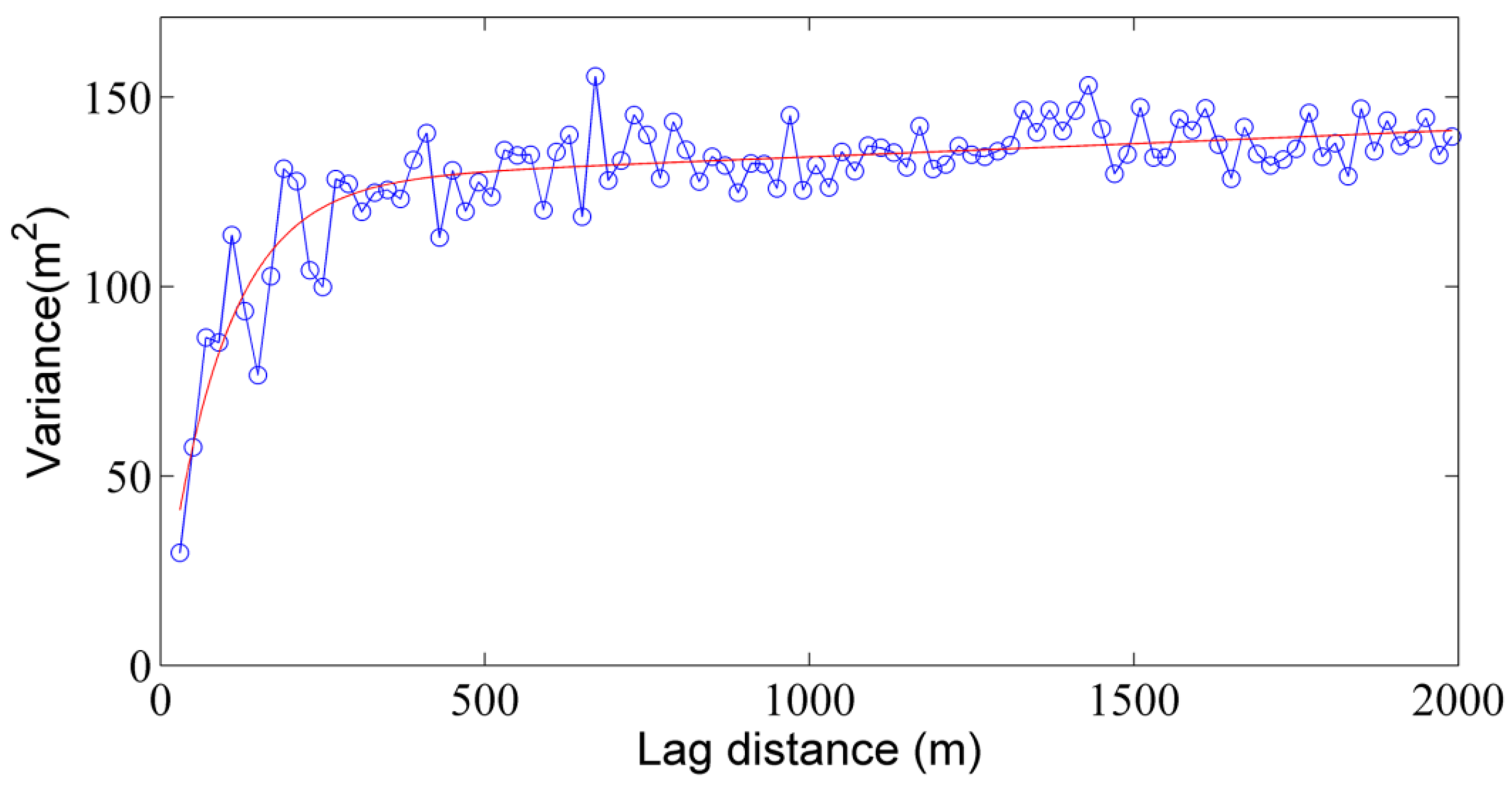
The uncertainty of volume change rate is calculated following [14] by Equation 5, where ${\mathrm{\sigma }}_{\mathrm{v}}’$ is the uncertainty of total volume change and N is the effective number of observations [40]. ${\mathrm{\sigma }}_{\mathrm{v}}’$ is obtained by multiplying the ${\mathrm{\sigma }}_{\mathrm{m}}$ by area. N is calculated using Equation 6 where ${\mathrm{N}}_{\text{tot}}$ is the total number of measurements. PS represents the pixel size and d is the distance of spatial correlation, which we have estimated as 400 m (Figure 7). The uncertainty of volume change rate estimation contributes a total uncertainty of approximately ±0.03 m·a⁻¹ to the final uncertainty of volume change for both glaciers.

$${\mathrm{\sigma }}_v=1.96\times \frac{{\mathrm{\sigma }}_v’}{\sqrt{N}}$$

(5)

$$N=\frac{N_{tot}\times PS}{2d}$$

(6)

Penetration of C-band radar waves can be a problem when using the SRTM DEM studying ice and snow. We are not able to perform the technique pioneered by [41], which compares the X-band SRTM elevations with C-band SRTM elevations, due to lack of X-band SRTM DEM coverage over our study areas. Instead, we generate a 4D DEM which has the same acquisition time (February 2000) as the SRTM DEM using tDEM, and subtract the actual SRTM DEM from our reconstructed DEM. We obtained an average −0.50 m and −0.26 m elevation difference for Fox Glacier and Franz Josef Glacier. We note that such differences could well originate from the penetration of C-band radar, expected to be small for southern hemisphere summer conditions, but also from fluctuation of glacier elevations. We do not have adequate data to conclude that such differences are solely due to C-band penetration, but rather incorporate them into the error budget. Thus, the penetration of the C-band SRTM DEM adds an additional uncertainty of approximately ±0.03 m·a⁻¹ and approximately ±0.02 m·a⁻¹ for Fox Glacier and Franz Josef Glacier, accordingly.

Finally, we account for a 10% error of area for the uncertainty budget [2]. All errors are summed quadratically on the condition that they are completely independent.

Figure 7. Semivariogram of elevation difference between ASTER DEM 2002/02/07 and the SRTM DEM, showing the decorrelation length (lag distance) from which the curve becomes “flattened”. An average decorrelation length of 400 m is estimated over all ASTER DEMs.

Figure 7. Semivariogram of elevation difference between ASTER DEM 2002/02/07 and the SRTM DEM, showing the decorrelation length (lag distance) from which the curve becomes “flattened”. An average decorrelation length of 400 m is estimated over all ASTER DEMs.

4. Results

4.1. Glacier Elevation Changes

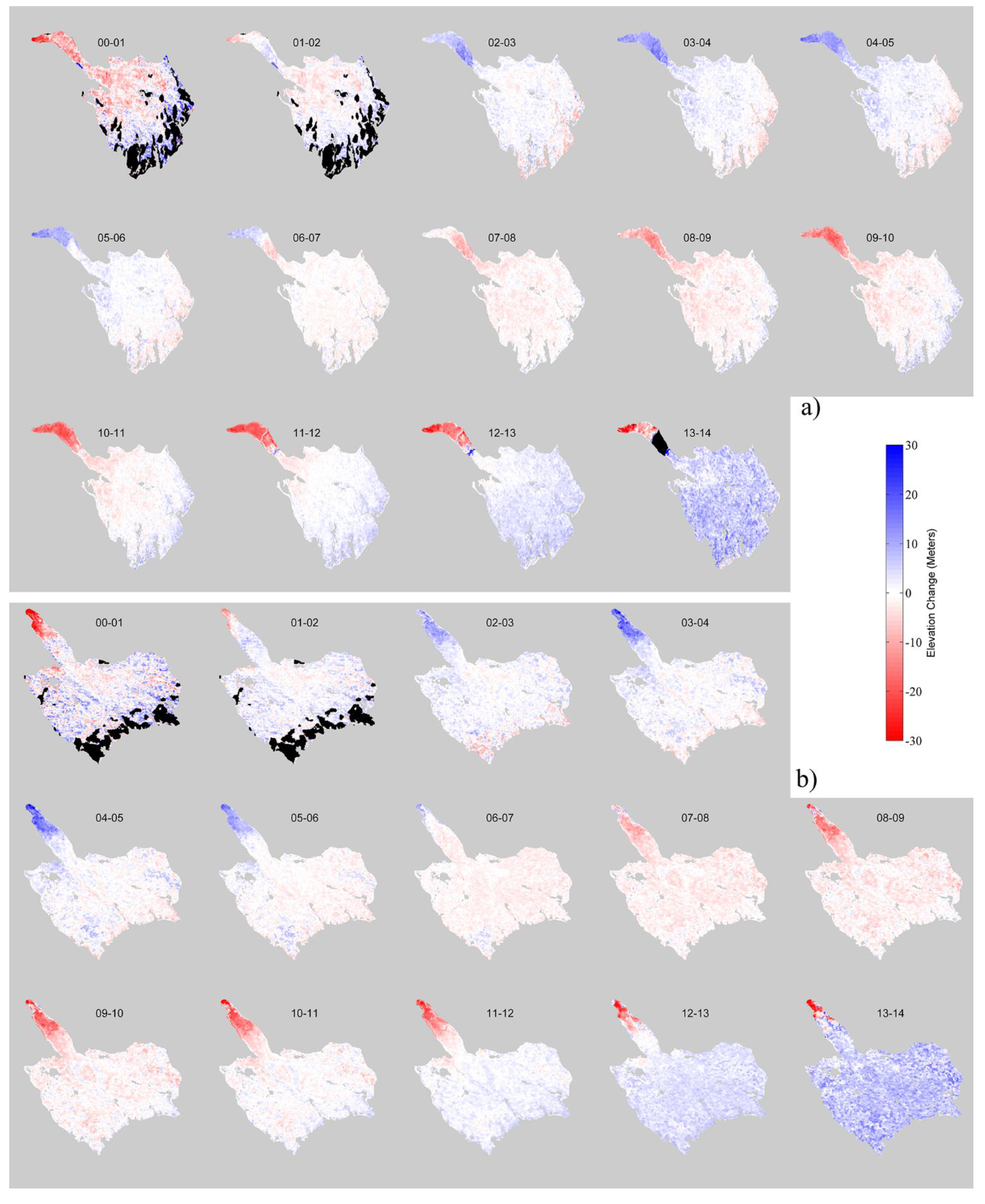
The map of annual elevation change of the two glaciers studied between 2000 and 2014 is given in Figure 8. We obtained an annual (calendar year) average dh/dt of −0.51 ± 0.02 m·a⁻¹ and −0.09 ± 0.02 m·a⁻¹ over the study period for Fox and Franz Josef Glacier, respectively. For reference, we extend our elevation change calculation back to 1986 by including the national DEM from 1986 air photos (Table 1). The elevation change rates between 1986 and 2000 are simply calculated by subtracting the national DEM from the SRTM DEM (Figure 5). We obtain an average surface lowering rate of −0.17 ± 0.01 m·a⁻¹ for Fox Glacier and a slightly positive surface elevation change of +0.04 ± 0.02 m·a⁻¹ for Franz Josef Glacier between 1986 and 2000. (Note that these estimates do not account for potential penetration of the SRTM C-band radar into the ice and snow).

Figure 8. Annual elevation change of (a) Fox Glacier (b) Franz Josef Glacier, modelled by the tDEM method from DEM time series data. Untrusted results due to missing data at the boundaries of the time series are marked with black. Time periods refer to calendar years, i.e., between 1 January of both years.

Figure 8. Annual elevation change of (a) Fox Glacier (b) Franz Josef Glacier, modelled by the tDEM method from DEM time series data. Untrusted results due to missing data at the boundaries of the time series are marked with black. Time periods refer to calendar years, i.e., between 1 January of both years.

4.2. Glacier Volume Changes

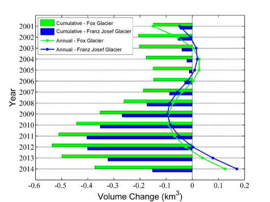
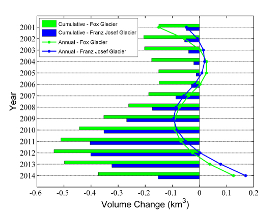
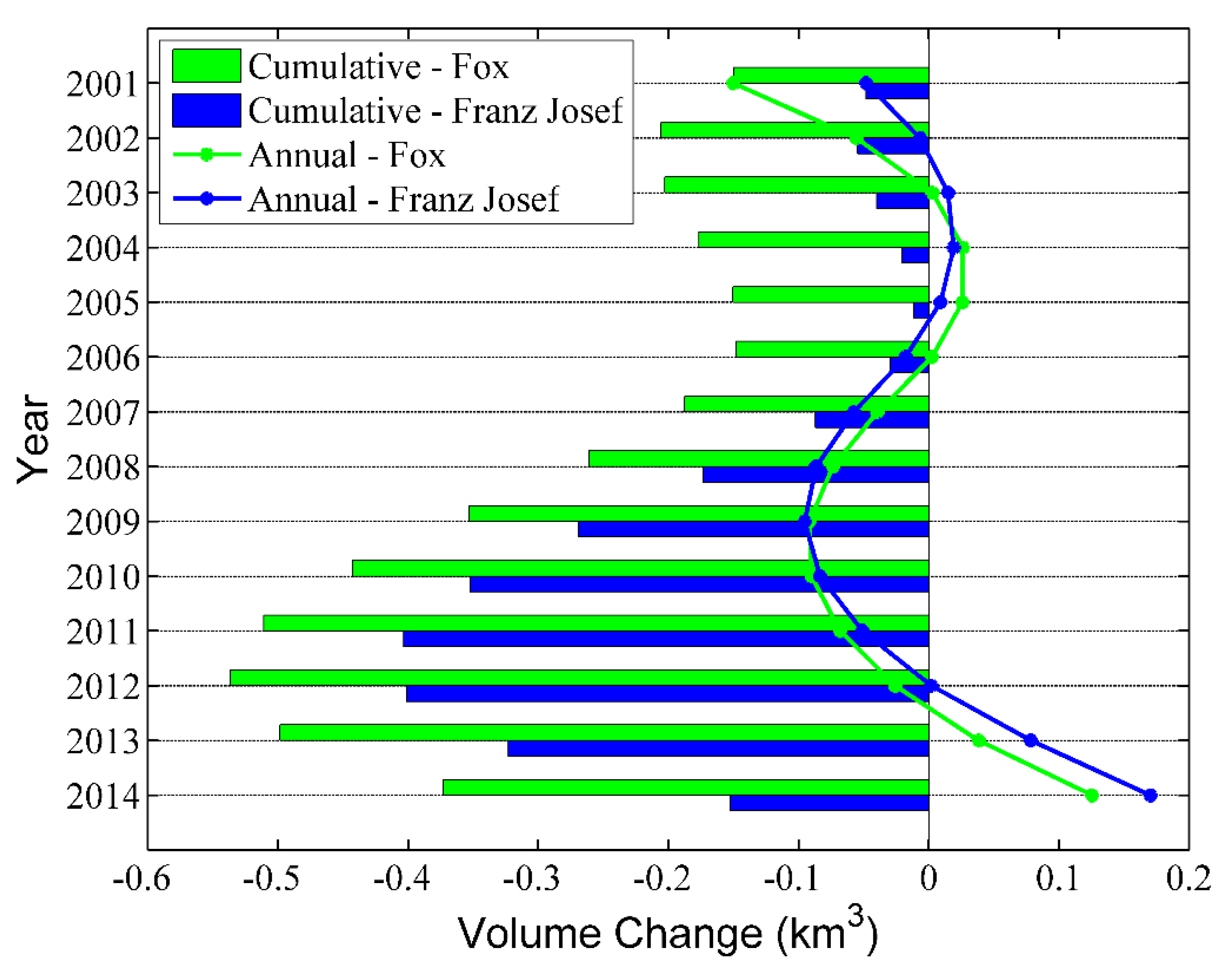
The volume changes were obtained from the reconstructed DEM time-series. We computed annual (calendar years) and cumulative volume change from 2000 to 2014 (Figure 9). The specific cumulative volume changes yield −0.77 ± 0.13 m·a⁻¹ and −0.33 ± 0.06 m·a⁻¹ for Fox and Franz Josef Glacier accordingly between 1 Jan 2000 and 1 Jan 2014. Note that these volume changes are calculated as the difference between two reconstructed DEMs divided by the number of years between the two DEMs, whereas the above average dh/dt (−0.51 ± 0.02 m·a⁻¹ and −0.09 ± 0.02 m·a⁻¹) are the average of all annual elevation changes over a period calculated from the derivatives of the fitted curves of elevation variation. As the differencing of two reconstructed (or real) DEMs disregards any elevation variation between the two dates, in contrast to the average dh/dt, the difference between the two sets of values reflects mainly different errors and error propagations (see also Section 5.1).

Figure 9. Annual (dot line) and total (bar) volume change of Fox Glacier (green) and Franz Josef Glacier (blue) between 2000 and 2014. The year in the Y-axis refers to 1 January of the ending year.

Figure 9. Annual (dot line) and total (bar) volume change of Fox Glacier (green) and Franz Josef Glacier (blue) between 2000 and 2014. The year in the Y-axis refers to 1 January of the ending year.

Fox Glacier gained volume between 2003 and 2006, and then again since 2013. Franz Josef Glacier showed a similar behavior, but tended to lead the change by approximately one year ahead of the Fox Glacier. Both glaciers lost most volume around the year 2009. The extended volume change between 1986 and 2000 is estimated as −0.17 ± 0.05 m·a⁻¹ and 0.0 ± 0.04 m·a⁻¹ for Fox Glacier and Franz Josef Glacier accordingly. Notably, Franz Josef Glacier has a similar volume in 1986 and 2000 (neglecting SRTM C-band penetration). Our results show that both glaciers are changing volume on average at a moderate rate, while other publications report that glaciers in the Southern hemisphere (South America) are losing mass more rapidly than the global average rate (e.g., [3,13,14]). The two glaciers studied seem to respond rapidly to changes in meteorological or glacier-internal conditions, presumably also in connection with their high rates of mass turn-over, steep mass-balance gradient, and hypsography with a large flat accumulation area and a steep narrow tongue, so that they are able to fluctuate significantly in elevation over just a few years. We have detected volume gain after 2012/2013, which in sum leads to a more moderate mass loss between 2000 and 2014, compared to, for instance, 2006–2010.

5. Discussion

5.1. tDEM Method

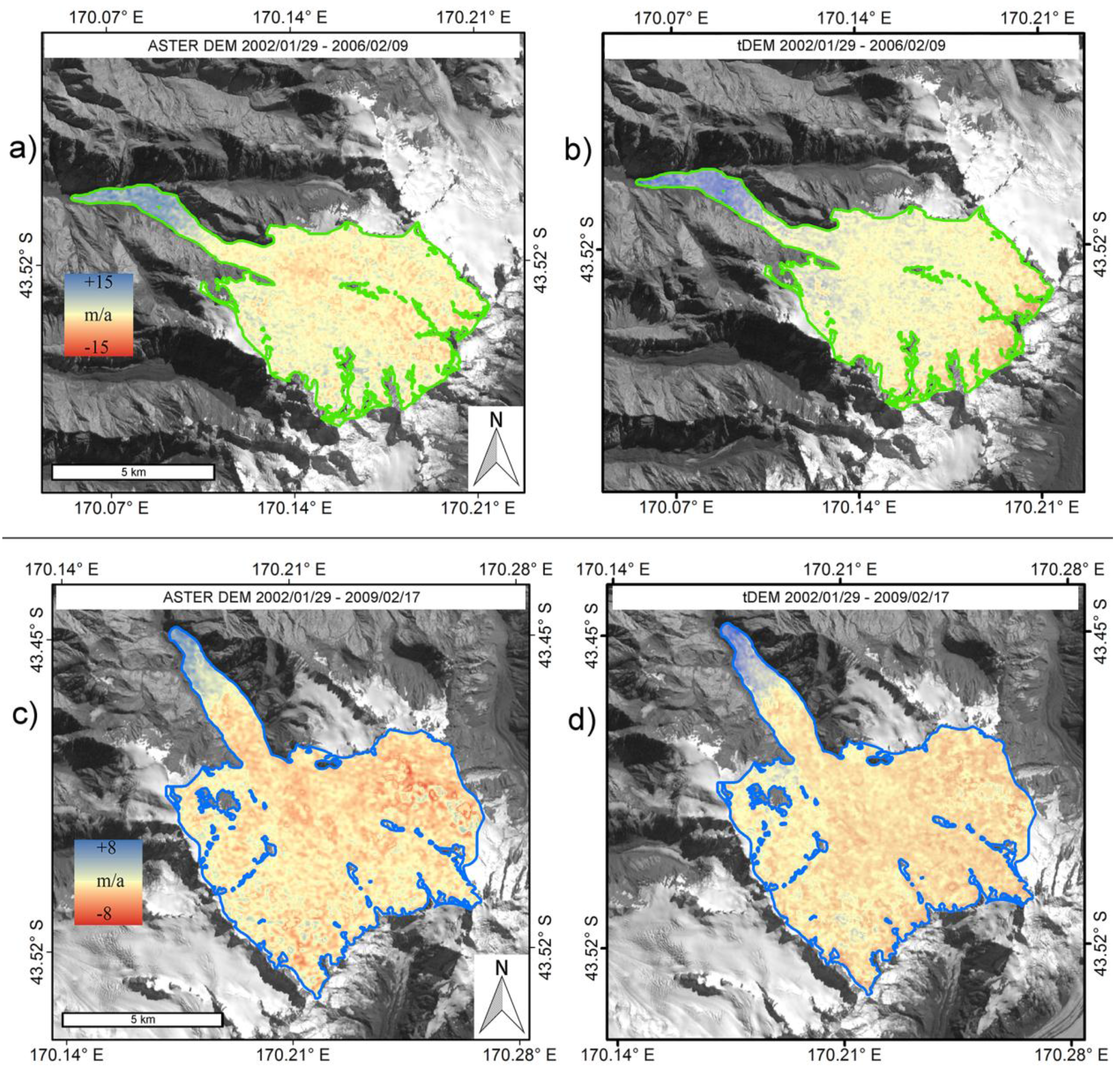
We have presented a method for DEM time series (tDEM), which calculates glacier elevation change rates by using the first derivative of modelled elevation change curves, and estimates volume change from the reconstructed 4D DEM. To date, available methods use approaches such as linear regression (e.g., [3,13,14]) and differencing between two DEMs (e.g., [4,11,28]) to quantify vertical glacier changes. Our method exploits time stacks of DEMs and is able to estimate non-linear developments of glacier elevation. As case studies, we calculated the volume change of two nearby glaciers by a simple linear regression method and DEM subtraction for comparison. The linear regression estimated 6% (Fox Glacier) and 93% (Franz Josef Glacier) more negative volume change than the tDEM method. The reason is that linear regression assumes the elevation is changing linearly, whereas we have shown that for the two glaciers a strong variation of elevation change rate existed (Figure 8 and Figure 9). Around 2002–2006 the glaciers studied showed a slight volume gain, and 2006–2012 a strong loss. Especially, a significant volume gain is identified after the year 2013, which gets a low weight in the linear regression due to its short time period in our DEM series. The subtraction between two ASTER DEMs of 2001 and 2014 did not reveal useful results due to a large proportion of cloud coverage existing in the DEMs around the year 2014. This underlines the limitations of DEM subtractions. However, we selected by visual inspection two DEMs that contain less outliers for both glaciers. DEMs 2002/01/29 and 2006/02/09 were selected for Fox Glacier, while DEMs 2002/01/29 and 2009/02/17 were chosen for Franz Josef Glacier. We then calculated elevation differences (Figure 10) and compared them with the results from our tDEM method, reconstructed for the exactly same dates. The mean elevation difference of Fox Glacier is estimated as +0.45 ± 0.07 m·a⁻¹ between 2002 and 2006 by traditional DEM subtraction of the two actual ASTER DEMs, while tDEM reveals +0.38 ± 0.02 m·a⁻¹ as mean difference between two DEMs reconstructed for the same dates as the two original ASTER DEMs. Similar compliance has also been found for Franz Josef Glacier, for which direct DEM subtraction results in −0.77 ± 0.03 m·a⁻¹ between 2002 and 2009, and tDEM estimates a lowering rate of −0.81 ± 0.02 m·a⁻¹ over the same time period from subtraction of reconstructed DEMs.

To further validate the reconstructed 4D DEM we have run the tDEM method to the same date as the acquisition of the SRTM DEM in February 2000, but without including the SRTM DEM in the curve fitting, and compared the reconstructed DEM with the original SRTM DEM. Mean elevation differences of −0.50 m and −0.26 m (with the original SRTM DEM being lower) are achieved for Fox Glacier and Franz Josef Glacier, respectively. The small deviation also suggests that our method is able to model the actual elevation evolution well.

The tDEM method detects and excludes outliers in elevation data by a two-category strategy; extreme elevation change limitations and the RANSAC filtering. That is, our method excludes outliers before the dh/dt is calculated, unlike studies that apply post-processing technique such as threshold filters based on standard deviations to optimize results. We consider our method is less influenced by spurious elevations than post-processing approaches. When reconstructing annual elevation changes, we iteratively approach a simple plane to the local surface for detecting outliers and replace them by local mean elevation change values. The simple approximation works well for detecting large blunders, potentially caused by incorrect curve fitting due to DEM errors.

Figure 10. (a) Elevation change on Fox Glacier from differencing of ASTER DEMs of 2002 and 2006. (b) Difference of two reconstructed DEMs of the same dates. (c) Elevation change on Franz Josef Glacier from ASTER DEMs of 2002 and 2009. (d) Difference of two reconstructed DEMs of the same dates. Underlying ASTER image of 2006/02/09. Both glaciers show slight thickening at the fronts.

Figure 10. (a) Elevation change on Fox Glacier from differencing of ASTER DEMs of 2002 and 2006. (b) Difference of two reconstructed DEMs of the same dates. (c) Elevation change on Franz Josef Glacier from ASTER DEMs of 2002 and 2009. (d) Difference of two reconstructed DEMs of the same dates. Underlying ASTER image of 2006/02/09. Both glaciers show slight thickening at the fronts.

The tDEM method controls the temporal data distribution by selecting one elevation per pixel (median) for each half year. In this way, the redundancy of temporal data makes the elevation data more robust. For example, six DEMs between 2012 and 2013 are incorporated in our study (Figure 4), making the final elevation of 2012–2013 more plausible even if some of the six DEMs contain a large amount of spurious elevations.

As for many curve fitting methods, our fitting of elevation evolution into elevation time series is somewhat sensitive to outliers at the beginning or end of the series (cf. Figure 5). The reconstructed tDEMs for 2000 and 2014 and thus the elevation changes including these years could thus be slightly offset. On the other hand, the above comparison of a reconstructed tDEM for 2000 with the SRTM DEM does not point to a big problem of this kind, at least towards the beginning of the series. An average dh/dt calculated as the mean of annual derivatives of the fitted curves over the entire period is only to a limited extent affected by such margin effects, and less than the differencing of two reconstructed 4D DEMs for dates at the margins of the time series.

5.2. Seasonal Variations and DEM Timing

As the focus of this contribution is mainly on discussing a method for assessing multi-annual time series of medium resolution satellite-derived DEMs, we did not pay close attention to seasonal variations of glacier elevation (See [42,43] for a discussion of the problem). The most important variation for the high-precipitation glaciers used here as example (precipitation up to 10 m·a⁻¹ water equivalent in the accumulation areas) is most likely snow. It could in theory well be that the volume variations found (Figure 8 and Figure 9) are to an unknown extent influenced by snow heights (or seasonal density changes) at the dates of data acquisition rather than changes in glacier mass. We tried to minimize this effect by three measures: first, all DEMs have been vertically co-registered so that the influence of varying snow thickness is removed to the extent to which average off-glacier snow thickness is representative for average on-glacier snow thickness. Second, using a median elevation for temporal groups with several DEMs available (see above) also reduces the effect of snow thickness to some extent. Third, our tDEM curve fit reduces through smoothing the influence of individual DEMs and thus of random component of variations of snow thickness, or acquisition timing.

To the best of our knowledge, no representative snow height measurements are available for the two glaciers, we cannot directly assess this influence strictly. While the ASTER DEMs used (or their mean date, respectively, for groups of DEMs) between 2002 and 2011 stem mostly from around January and February, the ones of 2001 and 2012–2014 from March or April. As the minimal snow cover (and the end of the balance year) for average conditions for the study region is around the latter time of the year [19,44], we should roughly expect decreasing snow (and glacier) surface heights from Jan/Feb to Mar/Apr. Based on this very rough overall estimate, the reduced glacier volume in 2001 could in fact be due to seasonal variations in snow thickness. The increasing glacier volume after ~2012, however, cannot be explained in a simple way by average seasonal variations in snow cover. Though, it is clear that singular snow events under the heavily maritime environment covered can have a big impact but are not covered sufficiently by the above general assumption of seasonal snow height variation.

In parts, the timing of DEMs and the snow cover percentages, if accepting the latter as indicator for snow thickness, show agreement (Figure 4) suggesting that there are partially systematic variations of snow cover with time contained in our DEM data set.

Besides the above general considerations and compensations, we prefer to not correct our DEMs for snow height (and other seasonal variations in height) in a more sophisticated way. The ground data necessary to establish a reliable seasonal variation of glacier height over the two glaciers investigated are not available to us. The heavy maritime character of the glaciers, the year-round high precipitation rates, and the weak annual variations of temperature may cause strong variability in snow heights, and thus make corrections based on average conditions questionable. Furthermore, we suggest that satellite-derived DEMs from medium resolution optical data (here: ASTER) are less sensitive to snow height variations than those from high-resolution data or even airborne laserscanning [42,43], as the reduced image resolution and the large windows needed for parallax matching (several 15 m × 15 m) is expected to capture mainly large-scale topographic features. Filling, or depletion, of small topographic depressions such as crevasses with snow should thus have little or at least reduced influence on elevation values obtained compared to high-resolution methods.

In further more glaciologically oriented applications of tDEM methods, seasonal height variations could be corrected for, provided sufficient data or models are available. In addition, our method can be optimized to reduce related effects, for instance by limiting the annual time frame of DEMs used to around maximal ablation conditions instead of using all suitable DEMs and calculating simple medians for seasonal groups of DEMs. It has to remain open and is not the focus of this multi-annual rather than seasonal study to what extent medium-resolution ASTER DEMs could even resolve seasonal variations in glacier height and volume.

Closely related to the above discussion about seasonal influences is the question which timing of the year our annual 4D DEM actually represents as it consists of DEMs from variable dates. The average acquisition date of the ASTER DEMs used is 21 March. This date overlaps well with the assumed date of maximal ablation over the study area and thus the start/end of the glacier mass balance year [19,44]. That means that our curves of elevation variation with time, and thus also our reconstructed 4D DEMs reflect on average maximum ablation conditions. Elevations given for the start of the calendar years, or elevation differences between calendar years, reflect thus for the most part mass balance years, with two limitations, though. First, as discussed in detail above, if the variations in acquisition days-of-the-year are systematically accompanied by variations in snow heights (Figure 4) and if these dates are not randomly distributed and thus eliminated by the fitting, a temporal bias in acquisition timing could lead to a temporal bias in reference date for the fitted elevation variations. Second, the elevations reconstructed are hypothetical as they do not contain seasonal variations. Even these ‘long-term’, non-seasonal elevation variations modelled here will to some extent depend on the exact interpolation date, though much less than seasonal elevation variations. As we give in most cases elevations for the calendar year, and not the actual mass balance year, the ‘long-term’, non-seasonal elevation change between 1 January and the average DEM timing (here 21 March) is neglected, but considered small for the about 2.5 months (see Figure 9).

5.3. Glacier Change

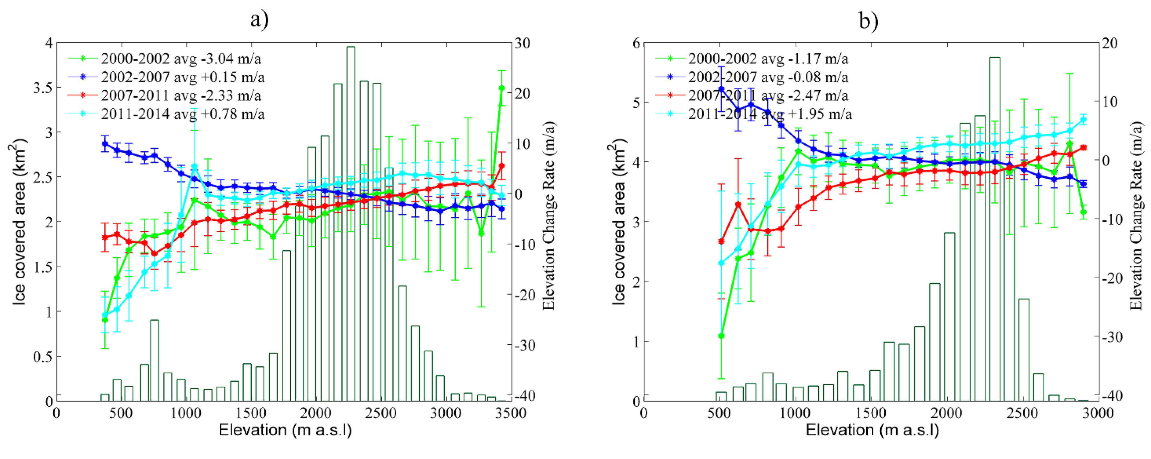
Under the neglect of seasonal variations as outlined above, we have shown that both Fox Glacier and Franz Josef Glacier experienced strong elevation fluctuations between 2000 and 2014. We divide the full observation period into four sub-periods, 2000–2002, 2002–2007, 2007–2011 and 2011–2014 based on the elevation change patterns found (Figure 8). Figure 11 shows the dh/dt versus glacier hypsometry in each of these sub-periods. Given that the two glaciers show similar elevation behavior, we take Fox Glacier as an example. Figure 8a indicates that the accumulation region was slightly thinning before 2002, followed by the thickening of the terminus between 2002 and 2008. At the same time, the accumulation zone lowered at high elevations. Our time series of 14 years is however too short to tell for sure if these seesaw-like thinnings and thickenings in the accumulation and ablation zones directly correspond to each other, or if the behavior of the tongue is actually in response to mass changes before 2000, or due to ice dynamical changes. Seasonal snow cover variations in the data would shift the curves mainly in the accumulation areas but leave the general pattern of contrasting elevation variation with elevation.

Authors in [15] report detailed length records for Fox Glacier and Franz Josef Glacier since the 1800s, which provides a reference for assessing our reconstructed elevations. Our elevation change results are in good agreement with their records of terminus positions. They point out that both glaciers were advancing between 2004 and 2008, while our results show that both glaciers were thickening at their termini within roughly the same time period. Our estimated moderate volume changes between 1986 and 2000 are also reasonable when compared with modelled time-series mass balance using a degree-day model [25].

Figure 11. Hypsometry and rate of glacier elevation change versus elevation on (a) Fox Glacier (b) Franz Josef Glacier. The colored lines represent the dh/dt estimated for each 100 m elevation bin, plotted with their corresponding standard deviations as error bars.

Figure 11. Hypsometry and rate of glacier elevation change versus elevation on (a) Fox Glacier (b) Franz Josef Glacier. The colored lines represent the dh/dt estimated for each 100 m elevation bin, plotted with their corresponding standard deviations as error bars.

For the New Zealand Southern Alps equilibrium line observations are used to estimate the mass balance of selected small and medium-size glaciers (Fox and Franz Josef Glaciers not included) [19,44]. These variations coincide reasonably well with our elevation changes, with some years of positive balances at and before 2005, and negative ones before and after until 2012 (time series available until 2013). Modelled mass balances for Franz Josef Glacier between 2000 and 2005 [20] give positive mass balances for all years except 2000/2001, which is also in line with our findings (Figure 9).

Authors in [25] measure glacier velocities on Fox and Franz Josef Glaciers based on correlation of seasonal ASTER image pairs in 2002 and 2006. They find velocity increases of roughly up to 150%–250% between 2002 and 2006, in particular on the termini, and compare these results to length and thickness changes at the glacier snouts. Our tDEM results agree also well with their study and further work cited in it; over 2001–2005 an increasingly positive mass balance was modelled for Franz Josef Glacier; between 2002 and 2006 Franz Josef Glacier thickened up to 70–80 m over the lowermost kilometer; both glaciers retreated from about 2000 to 2005 and advanced thereafter.

6. Conclusions

This paper described a methodology to reconstruct glacier elevation change from DEM time-series (tDEM). After initial removal of large outliers, either in relation to a reference DEM or using the RANSAC algorithm, the method generates a 4D DEM by fitting an elevation change development at each DEM pixel. The method tests progressively if linear, quadratic and cubic elevation developments are statistically significant and chooses a final robust spline fit if not. For the large majority of points on the particular study glaciers, linear to cubic fits did not produce significant curves, indicating a more complex pattern of elevation changes over the study region and time period. Glacier elevation change rates are then directly derived as the first derivatives of the fitted curves for each pixel. Glacier volume changes are obtained by subtracting the reconstructed time-dependent DEMs.

As a case study, we used 31 ASTER DEMs from 2001 to 2014 and the SRTM DEM over Fox Glacier and the Franz Josef Glacier in New Zealand. The quality of the generated 4D DEM was validated by comparing the SRTM DEM with a reconstructed tDEM at the SRTM acquisition time. Only small disparities were found (0.5 m and 0.26 m), indicating that our tDEM method is able to model and reconstruct the glacier elevation well. We also compared the tDEM with other, traditional approaches; DEM subtraction and linear regression. Linear regression gave a stronger glacier shrinking, likely because it could not sufficiently represent a recent volume gain at the end of our time series. DEM subtraction attempts did not give reasonable results over the same study timescale (2000–2014) due to the large fraction of cloud coverage and corresponding large DEM errors in individual ASTER DEMs. However, we calculated DEM subtraction between 2002 and 2006 (Fox Glacier), 2002 and 2009 (Franz Josef Glacier) from available good DEMs. For these optimal DEMs, the differencing results were in good agreement with tDEM over the same study periods. This suggests that our method of reconstructing the evolution of glacier elevation from DEM time series seems to work similarly well as the traditional method of DEM differencing where optimal DEM data are available, whereas our method is able to compensate for reduced DEM quality by statistical means incorporating a large number of DEMs.

We estimated an average annual glacier surface lowering rate of −0.51 ± 0.02 m·a⁻¹ and −0.09 ± 0.02 m·a⁻¹ between 2000 and 2014 for Fox Glacier and Franz Josef Glacier, respectively. The specific volume difference between two DEMs reconstructed for 2000 and 2014 by the tDEM method was calculated as −0.77 ± 0.13 m·a⁻¹ and −0.33 ± 0.06 m·a⁻¹. Our results agree reasonably well with published length change records and terminus thickness changes. Both glaciers show a rapidly changing spatio-temporal pattern of elevation changes.

Our tDEM method is able to cope with all kinds of elevation data, but particularly DEM data, because outlier removal and co-registration were so far optimized to handle gridded elevation data sets. The number and quality of worldwide available DEMs and other elevation data will continuously increase and so will the time periods covered. This calls for DEM time-series analysis approaches, and our study highlighted the potential and limitations of the methodology. The present work focused on multi-annual glacier volume changes from ASTER DEMs, i.e., medium resolution and medium quality data with, however, global availability. In the form demonstrated here, a limitation of our method is the handling of potential seasonal variations of glacier elevation. Related influences are reduced by several measures and circumstances but are not explicitly modelled. Another next development step of our tDEM approach should be the inclusion of data with different characteristics, such as optical stereo DEMs other than ASTER, or laser scanning and altimetry. It is clear that a number of variations and adaptations to our methodology are possible or even advisable when using different input data or applying it to different glaciological settings and tasks.

References

- Kääb, A.; Berthier, E.; Nuth, C.; Gardelle, J.; Arnaud, Y. Contrasting patterns of early twenty-first-century glacier mass change in the Himalayas. Nature 2012, 488, 495–498. [Google Scholar] [CrossRef] [PubMed]
- Kropáček, J.; Neckel, N.; Bauder, A. Estimation of mass balance of the Grosser Aletschgletscher, Swiss Alps, from ICESat laser altimetry data and digital elevation models. Remote Sens. 2014, 6, 5614–5632. [Google Scholar] [CrossRef]
- Willis, M.J.; Melkonian, A.K.; Pritchard, M.E.; Ramage, J.M. Ice loss rates at the Northern Patagonian Icefield derived using a decade of satellite remote sensing. Remote Sens. Environ. 2012, 117, 184–198. [Google Scholar] [CrossRef]
- Berthier, E.; Arnaud, Y.; Kumar, R.; Ahmad, S.; Wagnon, P.; Chevallier, P. Remote sensing estimates of glacier mass balances in the Himachal Pradesh (Western Himalaya, India). Remote Sens. Environ. 2007, 108, 327–338. [Google Scholar] [CrossRef] [Green Version]
- Kääb, A. Remote Sensing of Mountain Glaciers and Permafrost Creep; Geographisches Institut der Universität Zürich: Zürich, Switzerland, 2005; Volume 48. [Google Scholar]
- Nuth, C.; Moholdt, G.; Kohler, J.; Hagen, J.O.; Kääb, A. Svalbard glacier elevation changes and contribution to sea level rise. J. Geophys. Res. Earth Surface 2010, 115. [Google Scholar] [CrossRef]
- Zwally, H.; Schutz, B.; Abdalati, W.; Abshire, J.; Bentley, C.; Brenner, A.; Bufton, J.; Dezio, J.; Hancock, D.; Harding, D. ICESat's laser measurements of polar ice, atmosphere, ocean, and land. J. Geodyn. 2002, 34, 405–445. [Google Scholar] [CrossRef]
- Moholdt, G.; Nuth, C.; Hagen, J.O.; Kohler, J. Recent elevation changes of Svalbard glaciers derived from ICESat laser altimetry. Remote Sens. Environ. 2010, 114, 2756–2767. [Google Scholar] [CrossRef]
- Berthier, E.; Schiefer, E.; Clarke, G.K.; Menounos, B.; Rémy, F. Contribution of Alaskan glaciers to sea-level rise derived from satellite imagery. Nat. Geosci. 2010, 3, 92–95. [Google Scholar] [CrossRef] [Green Version]
- Pieczonka, T.; Bolch, T.; Junfeng, W.; Shiyin, L. Heterogeneous mass loss of glaciers in the Aksu-Tarim catchment (central Tien Shan) revealed by 1976 kh-9 hexagon and 2009 SPOT-5 stereo imagery. Remote Sens. Environ. 2013, 130, 233–244. [Google Scholar] [CrossRef] [Green Version]
- Gardelle, J.; Berthier, E.; Arnaud, Y.; Kääb, A. Region-wide glacier mass balances over the Pamir-Karakoram-Himalaya during 1999–2011. Cryosphere 2013, 7, 1263–1286. [Google Scholar] [CrossRef] [Green Version]
- Nuimura, T.; Fujita, K.; Yamaguchi, S.; Sharma, R.R. Elevation changes of glaciers revealed by multitemporal digital elevation models calibrated by GPS survey in the Khumbu region, Nepal Himalaya, 1992–2008. J. Glaciol. 2012, 58, 648–656. [Google Scholar] [CrossRef]
- Willis, M.J.; Melkonian, A.K.; Pritchard, M.E.; Rivera, A. Ice loss from the Southern Patagonian Ice Field, South America, between 2000 and 2012. Geophys. Res. Lett. 2012, 39. [Google Scholar] [CrossRef]
- Melkonian, A.; Willis, M.; Pritchard, M.; Rivera, A.; Bown, F.; Bernstein, S. Satellite-derived volume loss rates and glacier speeds for the Cordillera Darwin Icefield, Chile. Cryosphere 2013, 7, 823–839. [Google Scholar] [CrossRef]
- Purdie, H.; Anderson, B.; Chinn, T.; Owens, I.; Mackintosh, A.; Lawson, W. Franz Josef and Fox Glaciers, New Zealand: Historic length records. Glob. Planet. Chang. 2014, 121, 41–52. [Google Scholar] [CrossRef]
- Schenk, T.; Csatho, B. A new methodology for detecting ice sheet surface elevation changes from laser altimetry data. IEEE Trans. Geosci. Remote Sens. 2012, 50, 3302–3316. [Google Scholar] [CrossRef]
- Schenk, T.; Csatho, B.; van der Veen, C.; McCormick, D. Fusion of multi-sensor surface elevation data for improved characterization of rapidly changing outlet glaciers in Greenland. Remote Sens. Environ. 2014, 149, 239–251. [Google Scholar] [CrossRef]
- Csatho, B.M.; Schenk, A.F.; van der Veen, C.J.; Babonis, G.; Duncan, K.; Rezvanbehbahani, S.; van den Broeke, M.R.; Simonsen, S.B.; Nagarajan, S.; van Angelen, J.H. Laser altimetry reveals complex pattern of Greenland ice sheet dynamics. Proc. Natl. Acad. Sci. USA 2014, 111, 18478–18483. [Google Scholar] [CrossRef] [PubMed]
- Chinn, T.J.; Kargel, J.S.; Leonard, G.J.; Haritashya, U.K.; Pleasants, M. New Zealand’s glaciers. In Global Land Ice Measurements from Space; Kargel, J.S., Leonard, G.J., Bishop, M.P., Kääb, A., Raup, B.H., Eds.; Springer-Verlag: Berlin/Heidelberg, Germany, 2014; pp. 675–715. [Google Scholar]
- Anderson, B.; Lawson, W.; Owens, I.; Goodsell, B. Past and future mass balance of 'Ka Roimata o Hine Hukatere' Franz Josef Glacier, New Zealand. J. Glaciol. 2006, 52, 597–607. [Google Scholar] [CrossRef]
- Anderson, B.; Mackintosh, A. Temperature change is the major driver of late-glacial and holocene glacier fluctuations in New Zealand. Geology 2006, 34, 121–124. [Google Scholar] [CrossRef]
- Anderson, B.; Lawson, W.; Owens, I. Response of Franz Josef Glacier Ka Roimata o Hine Hukatere to climate change. Glob. Planet. Chang. 2008, 63, 23–30. [Google Scholar] [CrossRef]
- Purdie, H.L.; Brook, M.S.; Fuller, I.C. Seasonal variation in ablation and surface velocity on a temperate maritime Glacier: Fox Glacier, New Zealand. Arctic Antarct. Alp. Res. 2008, 40, 140–147. [Google Scholar] [CrossRef]
- Oerlemans, J. Climate sensitivity of Franz Josef Glacier, New Zealand, as revealed by numerical modeling. Arctic Alp. Res. 1997, 29, 233–239. [Google Scholar] [CrossRef]
- Herman, F.; Anderson, B.; Leprince, S. Mountain glacier velocity variation during a retreat/advance cycle quantified using sub-pixel analysis of ASTER images. J. Glaciol. 2011, 57, 197–207. [Google Scholar] [CrossRef]
- Chinn, T.; Winkler, S.; Salinger, M.J.; Haakensen, N.S. Recent glacier advances in Norway and New Zealand: A comparison of their glaciological and meteorological causes. Geogr. Ann. Ser. A-Phys. Geogr. 2005, 87, 141–157. [Google Scholar] [CrossRef]
- Rabus, B.; Eineder, M.; Roth, A.; Bamler, R. The shuttle radar topography mission—A new class of digital elevation models acquired by spaceborne radar. ISPRS J. Photogramm. Remote Sens. 2003, 57, 241–262. [Google Scholar] [CrossRef]
- Nuth, C.; Kääb, A. Co-registration and bias corrections of satellite elevation data sets for quantifying glacier thickness change. Cryosphere 2011, 5, 271–290. [Google Scholar] [CrossRef]
- Rodriguez, E.; Morris, C.S.; Belz, J.E. A global assessment of the SRTM performance. Photogramm. Eng. Remote Sens. 2006, 72, 249–260. [Google Scholar] [CrossRef]
- Pfeffer, W.; Arendt, A.A.; Bliss, A.; Bolch, T.; Cogley, J.G.; Gardner, A.S.; Hagen, J.O.; Hock, R.; Kaser, G.; Kienholz, C.; et al. The Randolph Glacier Inventory: A globally complete inventory of glaciers. J. Glaciol. 2014, 60, 537–552. [Google Scholar] [CrossRef] [Green Version]
- Abrams, M. The advanced spaceborne thermal emission and reflection radiometer (ASTER): Data products for the high spatial resolution imager on NASA's Terra platform. Int. J. Remote Sens. 2000, 21, 847–859. [Google Scholar] [CrossRef]
- Gjermundsen, E.; Mathieu, R.; Kääb, A.; Chinn, T.; Fitzharris, B.; Hagen, J. Assessment of multispectral glacier mapping methods and derivation of glacier area changes, 1978–2002, in the central Southern Alps, New Zealand, from ASTER satellite data, field survey and existing inventory data. J. Glaciol. 2011, 57, 667–683. [Google Scholar] [CrossRef]
- Gardner, A.; Moholdt, G.; Arendt, A.; Wouters, B. Accelerated contributions of Canada’s Baffin and Bylot Island glaciers to sea level rise over the past half century. Cryosphere 2012, 6, 1103–1125. [Google Scholar] [CrossRef]
- Höhle, J.; Höhle, M. Accuracy assessment of digital elevation models by means of robust statistical methods. ISPRS J. Photogramm. Remote Sens. 2009, 64, 398–406. [Google Scholar] [CrossRef]
- Fischler, M.A.; Bolles, R.C. Random sample consensus: A paradigm for model fitting with applications to image analysis and automated cartography. Commun. ACM 1981, 24, 381–395. [Google Scholar] [CrossRef]
- Berthier, E.; Vincent, C.; Magnússon, E.; Gunnlaugsson, Á.; Pitte, P.; le Meur, E.; Masiokas, M.; Ruiz, L.; Pálsson, F.; Belart, J. Glacier topography and elevation changes derived from Pléiades sub-meter stereo images. Cryosphere 2014, 8, 2275–2291. [Google Scholar] [CrossRef]
- Lundgren, J. Splinefit, MATLAB Central File Exchange. Available online: http://www.mathworks.com/matlabcentral/fileexchange/13812-splinefit (accessed on 4 August 2015).
- De Boor, C. A Practical Guide to Splines; Springer-Verlag: New York, NY, USA, 1978. [Google Scholar]
- Grohman, G.; Kroenung, G.; Strebeck, J. Filling SRTM voids: The delta surface fill method. Photogramm. Eng. Remote Sens. 2006, 72, 213–216. [Google Scholar]
- Rolstad, C.; Haug, T.; Denby, B. Spatially integrated geodetic glacier mass balance and its uncertainty based on geostatistical analysis: Application to the Western Svartisen ice cap, Norway. J. Glaciol. 2009, 55, 666–680. [Google Scholar] [CrossRef]
- Gardelle, J.; Berthier, E.; Arnaud, Y. Impact of resolution and radar penetration on glacier elevation changes computed from dem differencing. J. Glaciol. 2012, 58, 419–422. [Google Scholar] [CrossRef]
- Fischer, A. Comparison of direct and geodetic mass balances on a multiannual time scale. Cryosphere 2011, 5, 107–124. [Google Scholar] [CrossRef]
- Helfricht, K.; Kuhn, M.; Keuschnig, M.; Heilig, A. Lidar snow cover studies on glaciers in the Ötztal Alps (Austria): comparison with snow depths calculated from GPR measurements. Cryosphere 2014, 8, 41–57. [Google Scholar] [CrossRef]
- Willsman, A.P.; Chinn, T.; Lorrey, A. New Zealand Glacier Monitoring: End of Summer Snowline Survey 2013; NIWA Report; CHC2014–022; NIWA: Christchurch, New Zealand, 2014. [Google Scholar]
© 2015 by the authors; licensee MDPI, Basel, Switzerland. This article is an open access article distributed under the terms and conditions of the Creative Commons Attribution license (http://creativecommons.org/licenses/by/4.0/).
Share and Cite
MDPI and ACS Style
Wang, D.; Kääb, A. Modeling Glacier Elevation Change from DEM Time Series. Remote Sens. 2015, 7, 10117-10142. https://0-doi-org.brum.beds.ac.uk/10.3390/rs70810117
AMA Style
Wang D, Kääb A. Modeling Glacier Elevation Change from DEM Time Series. Remote Sensing. 2015; 7(8):10117-10142. https://0-doi-org.brum.beds.ac.uk/10.3390/rs70810117
Chicago/Turabian StyleWang, Di, and Andreas Kääb. 2015. "Modeling Glacier Elevation Change from DEM Time Series" Remote Sensing 7, no. 8: 10117-10142. https://0-doi-org.brum.beds.ac.uk/10.3390/rs70810117