Luminance-Corrected 3D Point Clouds for Road and Street Environments

Abstract

A novel approach to evaluating night-time road and street environment lighting conditions through 3D point clouds is presented. The combination of luminance imaging and 3D point cloud acquired with a terrestrial laser scanner was used for analyzing 3D luminance on the road surface. A calculation of the luminance (cd/m²) was based on the RGB output values of a Nikon D800E digital still camera. The camera was calibrated with a reference luminance source. The relative orientation between the luminance images and intensity image of the 3D point cloud was solved in order to integrate the data sets into the same coordinate system. As a result, the 3D model of road environment luminance is illustrated and the ability to exploit the method for evaluating the luminance distribution on the road surface is presented. Furthermore, the limitations and future prospects of the methodology are addressed. The method provides promising results for studying road lighting conditions in future lighting optimizations. The paper presents the methodology and its experimental application on a road section which consists of five luminaires installed on one side of a two-lane road in Otaniemi, Espoo, Finland.

1. Introduction

The function of road and street environment lighting is to maintain safety and comfort by providing acceptable visibility conditions during the night-time. Design of new road lighting setups, and retrofitting of old ones is affected by energy efficiency requirements [1] and by the ban of mercury lamps [2]. The increased awareness of mesopic vision may also affect the design of road lighting (e.g., [3,4]). The measurements of traffic lighting conditions are used to evaluate the performance of the lighting installation on road surfaces, road markings and furniture, or the glare from luminaires on surrounding areas can be investigated. Lighting measurements are also necessary for maintenance purposes. In the future, LED lights will be used more and more for illuminating road environments, because the luminous efficacies of the most recent LED luminaires are higher than the majority of the traditional light sources. Therefore, it is also important to evaluate the performance of LEDs for illuminating roadways.

With conventional gas discharge lamp luminaires, it is common to design outdoor lighting using a lumen maintenance factor of 80%. Lumen depreciation is due to lamp lumen depreciation but also due to luminaires getting dirty. A lumen maintenance factor of 80% is suitable if lamps are replaced with group replacement after three or four years, with burning hours thus being 12,000 to 16,000 hours. With LED luminaires the situation is different: their operating life time varies from 50,000 to 100,000 hours according to the manufacturer’s information. However, the luminous flux of the LED chips is reduced during burning hours and the rate of depreciation is affected by the ambient temperature, for instance. In addition, air pollution effects on the lenses of the LED package and also on the external optics, thus reducing the luminous flux on road surface. Therefore, LED luminaires will bring about a new requirement for lighting measurements during burning hours in order to confirm that the LED lighting installation is still meeting the lighting needs after several thousand burning hours.

Road environment lighting conditions are evaluated using different methods, depending on the type of road or street: illuminance and its uniformity, luminance and its uniformity, glare restriction, target visibility, or color of the light. In this work, the lighting conditions are assessed in terms of luminance. Luminance describes the luminous intensity emitted from a particular area in a given direction. The SI unit for luminance is candela per square metre (cd/m²). Luminance of the road is determined by the surface reflection properties and the light intensity based on the direction of light and the angle of reflection. Luminance measurements of road and street environments are needed to get data for analyzing the quality of road lighting and visibility conditions, for example.

Road lighting measurements can be carried out with spot luminance meters, which measure the luminance of a small (usually 1°) area at a time or by using an imaging luminance photometer (e.g., [5]). Zhou et al. [6] measured lighting illuminance levels for a moving vehicle and matched the measurements with the location data from a distance measurement instrument.

In recent years, laser scanning (LS) instruments have provided efficient and versatile applications for collecting 3D data for built and natural environments. Combined with positioning techniques LS produces the georeferenced point cloud, from which it is possible to calculate various surface, raster, and object models. In road and street environments,a mobile laser scanning (MLS) point cloud has been used for extracting different features, such as building façades, road surfaces, tunnels, railway tracks, poles, luminaires, and trees (e.g., [7,8,9,10,11,12,13,14,15]).

The fusion of 3D point cloud and image texture improves the interpretation and detection of features and objects. When considering data fusion, both 3D point clouds and 2D images must be registered in the common coordinate frame. The main approaches to registration include determining the sensor orientations separately using ground control features, solving the relative orientation between data sets, or making a system calibration of the integrated imaging system [16]. The combination of 3D point clouds with other sensor techniques can be found in a large number of published works. For example, point clouds have been integrated with data from a thermographic camera and ground-penetrating radar [17,18,19]. The result can also be a georeferenced panorama image, a textured surface, a building façade or a virtual environment [20,21,22,23]. In addition, point cloud rendering methods are used to improve the visualization (e.g., [24]).

The objective of this study is to demonstrate a novel approach to create luminance-corrected 3D point cloud data for evaluating night-time road lighting conditions and to address the limitations and future prospects.

2. Study Area and Data Acquisition

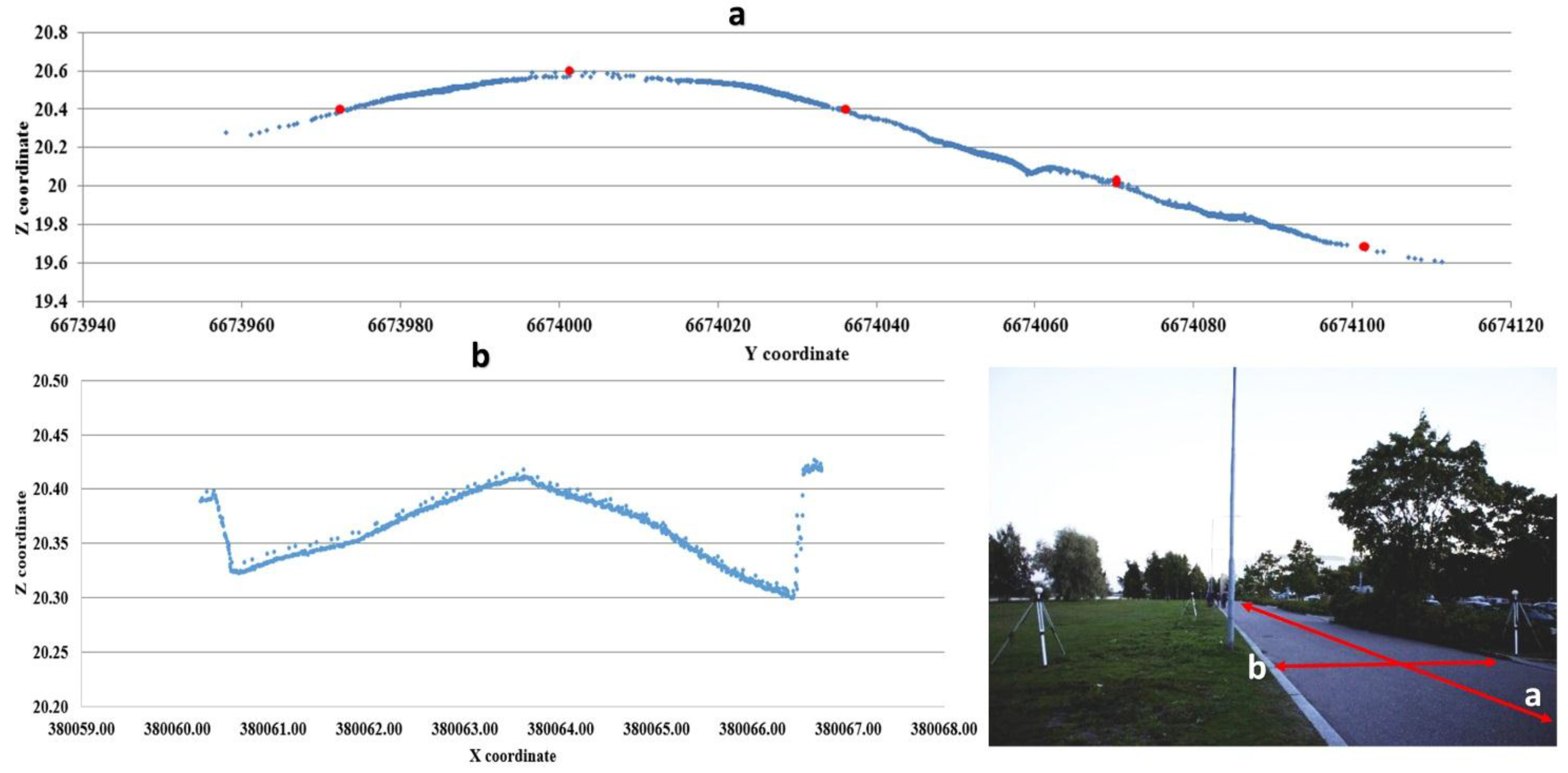
2.1. Test Site

The research was conducted on a straight street section in Otaranta, Espoo, Finland (Figure 1). The experimental road section was approximately 150 m long and 6 m wide. The road has 1% slope in the longitudinal direction and 3% cross-section slope in both lanes. The difference between the lowest and highest point of the road section was 1 m. The road is surrounded by lawns and parking areas. The road section consists of five luminaires installed on one side of a two-lane road. The spacing between the poles was 32 m, with the luminaire being mounted at height of 10 m. Each luminaire had one 100 W High Pressure Sodium (HPS) light source. The road surface is classified as R3 in the CIE road surface classification, with a lighting class of AL4b, which is similar to ME4b in European standards, except for the longitudinal uniformity.

2.2. 3D Point Cloud

We used a Faro Focus 3D terrestrial laser scanner to produce a 3D point cloud of the Otaranta road. The Faro Focus 3D is a 905 nm, phase-based, continuous-wave laser scanner with a 305° × 360° field of view. The distance measurement accuracy is ±2 mm at a distance of 25 m [25]. The circular beam diameter at the exit is 3 mm. In total, we measured the Otaranta road from four separate scanning positions which were located between the lamp posts. 3D data was acquired with a resolution setting, providing a point spacing of 6 mm on an orthogonal target located some 10 m from the scanner. The objective of the laser scanning measurements was to obtain the comprehensive point coverage for the road surface and its surroundings. The TLS point clouds were co-registered using at least three sphere reference targets between every scan pair. The distance between the sphere target and scanner remained reasonable relative to the scanning resolution used. In this study, the distances varied from 5 to 15 m. The spheres were positioned with VRS-GNSS measurements. The overall quality of the registration on reference targets showed 1.0 cm mean error. The output of the TLS measurements was then georeferenced using the Finnish ETRS-TM35 coordinate system. In total, 73 million points were measured from the area.

Figure 1. Profile view of the Otaranta road center line (a) and cross-section (b). Z coordinates are presented in GRS80 (Geodetic Reference System 1980), Y and X coordinates in ETRS-TM35FIN, units expressed in meters (positions of poles are marked with red dots in picture a).

Figure 1. Profile view of the Otaranta road center line (a) and cross-section (b). Z coordinates are presented in GRS80 (Geodetic Reference System 1980), Y and X coordinates in ETRS-TM35FIN, units expressed in meters (positions of poles are marked with red dots in picture a).

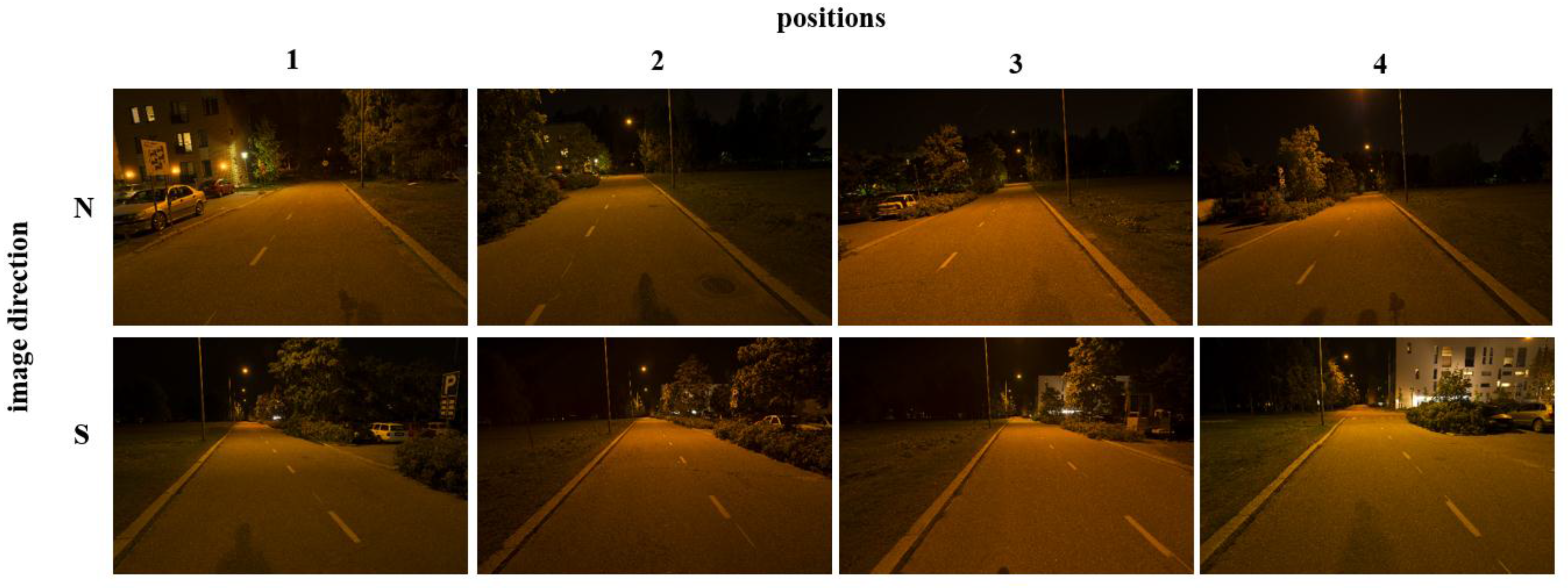
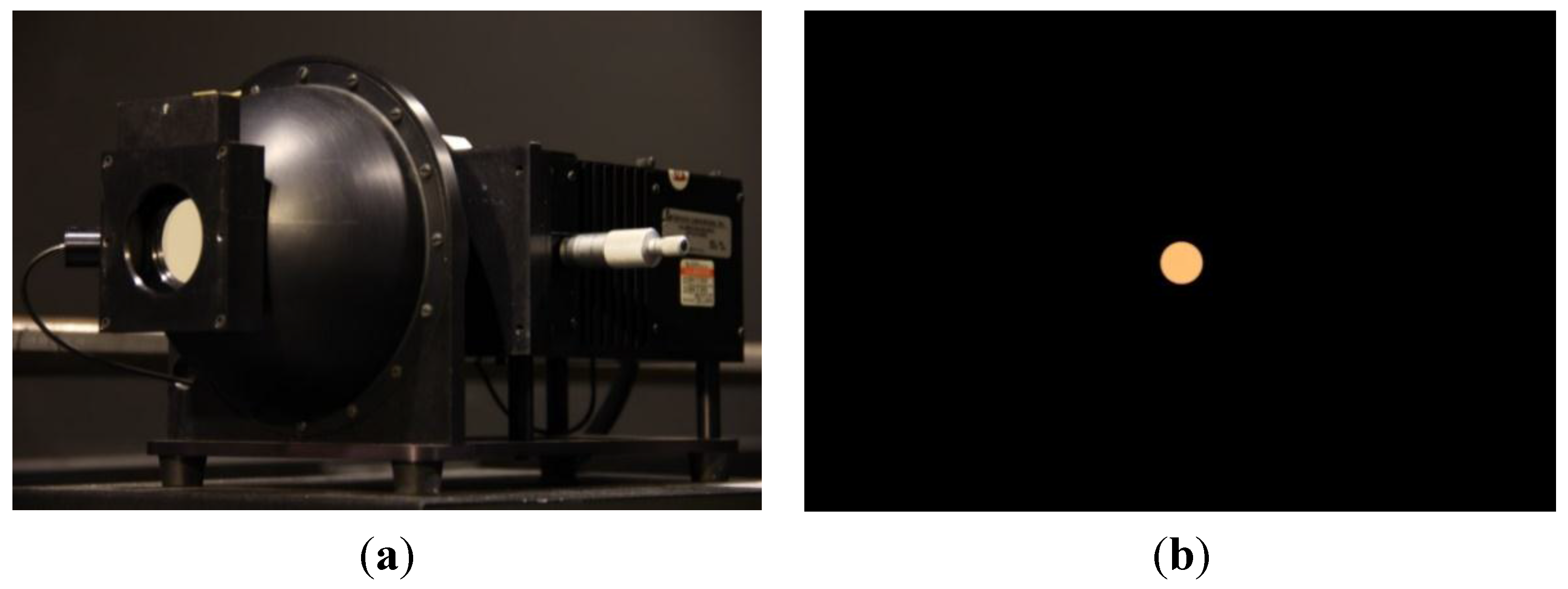
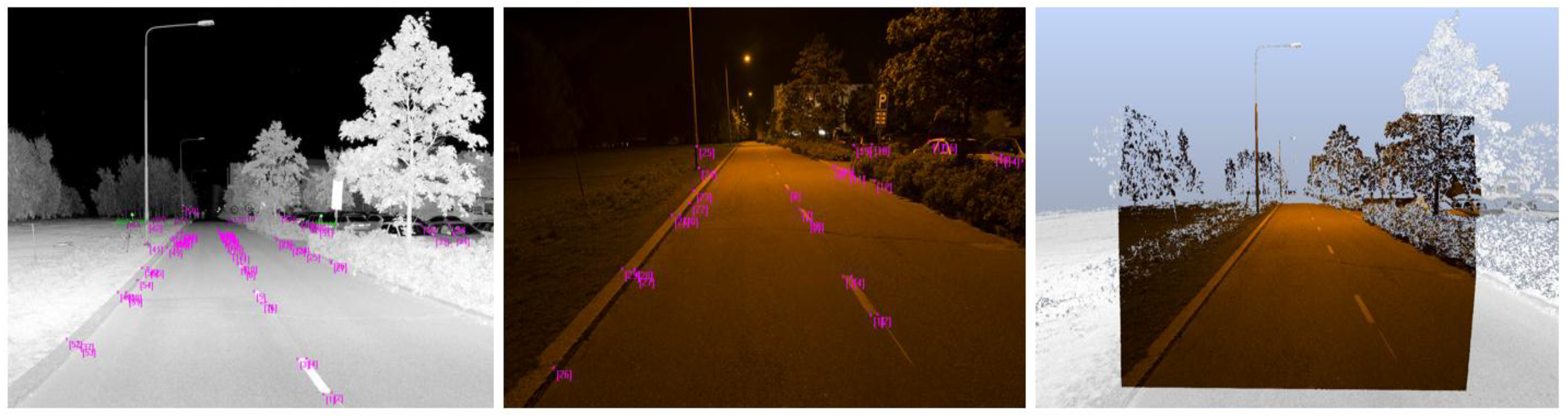
2.3. Image Acquisition

Image acquisition was performed from the same locations using the same tripod setup as with TLS scans and for both directions of the road with a Nikon D800E camera (Figure 2). For the camera, the field of view was similar to the driver’s point of view. The aperture of the camera was 5.6, exposure time 8 s and ISO value 100. These settings enabled luminance values of under 5 cd/m² with maximum dynamic range to be captured. All images were taken continuously under conditions where the existing luminance did not vary during the measurement. The photos were saved in NEF format (Nikon’s lossless RAW file format) to record light linearly and maximize image quality for post-processing.

To address a 3D point with an absolute luminance value, the absolute luminance value must first be clarified. A digital camera can be used as an imaging luminance photometer [26,27,28]. To interpret the images taken as matrices, the absolute luminance values of the pixel in the raw image of the camera used needed to be calibrated. In addition, the camera was geometrically calibrated and lens distortions were corrected by applying Brown’s model [29].

Figure 2. The image data included eight images covering a 150-metre long road section under night-time lighting conditions. The images were taken from four different positions and in both directions (north and south).

Figure 2. The image data included eight images covering a 150-metre long road section under night-time lighting conditions. The images were taken from four different positions and in both directions (north and south).

Luminance Calibration

For obtaining luminance values from digital images, Equations (1) and (2) are applied. The relation between aperture, exposure time, ISO, and luminance is explained in the following Equation [28]:

$$K=\frac{N_d{f}_s^2}{L_{s}t{S}_{ISO}}$$

(1)

where

• K is the calibration constants
• N_d is the digital value Y of the pixel in the raw image obtained with equation 2,
• f_s is the aperture,
• L_s is the luminance of the scene in cd/m²
• t is the exposure time in seconds and
• S_ISO is the ISO value.

The value of Y in the CIE XYZ color space [30] is equivalent to the photopic luminance value [31]. The correlation between the RGB color space used in the Nikon D800E camera and Y in CIE XYZ is defined by the IEC standard [32]:

$$Y=0.2162R+0.7152G+0.0722B$$

(2)

To determine the ratio of absolute and relative luminances with specific exposure settings, a set of images with known luminance were acquired. An Optronic Laboratories Inc. model 455-6-1 reference luminance source (Figure 3a) was used to create uniform circular luminance areas. To obtain low luminance values corresponding to night-time road conditions, a neutral density (ND) filter was used in front of the opening of the luminance source’s integrating sphere. The transfer ratio of the ND filter was measured using an LMK Mobile Advanced imaging luminance photometer, and found to be 1/41.8. After this, a series of 54 images of the ND-filtered luminance source were taken with the Nikon D800E. The calibration was performed with the same exposure settings as used in the field (aperture of the lens 5.6, exposure time of 8 s and the ISO value 100). The luminance source was adjusted to 54 different luminance ranging from 0.0031 to 23.95 cd/m². The median RGB channel values from an area of 100 × 100 pixels in the center of the image (Figure 3b) covering the opening of the luminance source were used in calibrating the camera.

Figure 3. (a) Optronic Laboratories Inc. model 455-6-1 reference luminance source used for calibration. (b) The image covering the opening of the luminance source.

Figure 3. (a) Optronic Laboratories Inc. model 455-6-1 reference luminance source used for calibration. (b) The image covering the opening of the luminance source.

Using the transformation function (Equation (2)) with an RGB image, a matrix of relative luminance values was obtained. With the absolute luminance value of the image being known, the linear ratio between relative and absolute luminance values was identified. It was found that with the exposure settings used, the maximum measurable luminance value was 2.9 cd/m² because, with greater values, one of the RGB channels reached its limits. The ratio and the RGB to Y function (Equation (2)) can now be used to interpret every image taken with the calibrated camera, using the same exposure settings, as a matrix of absolute luminance values.

3. Integration of Luminance Values and 3D Point Cloud

Our approach to derive a 3D luminance model for analyzing road environment lighting conditions is based on the fusion of TLS measurements and luminance values derived from digital images. The creation of luminance colored 3D point clouds requires that images and laser scanning data are in the same coordinate system. We integrated these terrestrial data sources by determining the orientation of undistorted RGB images relative to intensity images of individual terrestrial laser scans (Figure 4). We identified a set of corresponding points for every image pair by using recognizable road features such as paintings and kerbstones. The results of the registration showed that the mean distance between the 2D projection of the selected 3D points and the corresponding points that have been selected in the RGB pictures for all image pair was 4.7 pixels. The uncertainty was mainly caused by lower resolution on TLS intensity images. After determining the orientation, the images were replaced by calculated luminance images (see Section 2.3.1) in order to derive 3D luminance point clouds. The RGB images were used for orientation for the reason that they allowed us to observe the road features more clearly.

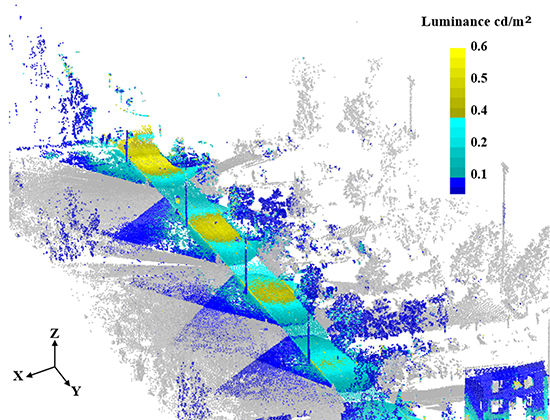
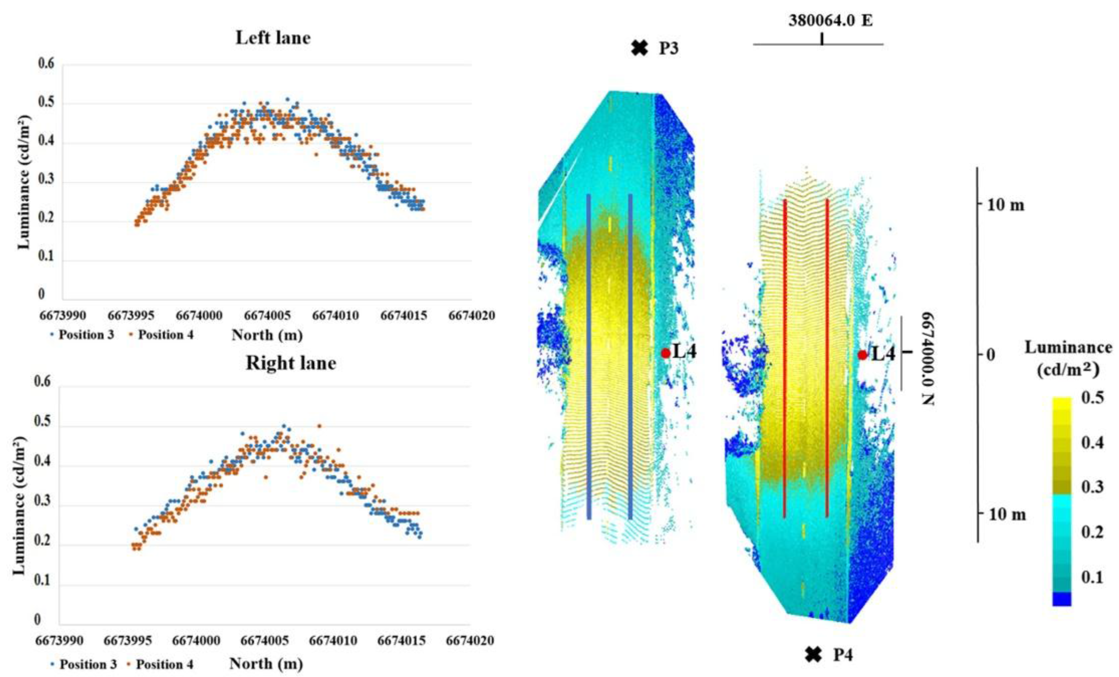
3.1. 3D Luminance Point Cloud

Once all images have been registered with the corresponding TLS intensity images, the 3D luminance data of the road can be generated. In other words, every measurement point contains x, y, and z coordinates and a calibrated luminance value. The output is that individual TLS scans are textured with two images covering both directions of the road. That enabled us to obtain comprehensive point coverage for the studied road surface. The perpendicular directions along the road were not evaluated in this study. The output is presented in Figure 5.

Figure 4. Road features such as paintings and kerbstones were used as corresponding points between a TLS-based intensity image and an RGB image for resolving the relative orientation.

Figure 4. Road features such as paintings and kerbstones were used as corresponding points between a TLS-based intensity image and an RGB image for resolving the relative orientation.

Figure 5. The derived 3D luminance data of the road section; (a) bird’s-eye view and (b) orthographic view, from above. The points which are not textured by images are shown in grey. The positions of the scan and image stations are marked with black crosses (P1–P4) and lamp posts are marked with red dots (L1–L5). Coordinates are presented in ETRS-TM35FIN.

Figure 5. The derived 3D luminance data of the road section; (a) bird’s-eye view and (b) orthographic view, from above. The points which are not textured by images are shown in grey. The positions of the scan and image stations are marked with black crosses (P1–P4) and lamp posts are marked with red dots (L1–L5). Coordinates are presented in ETRS-TM35FIN.

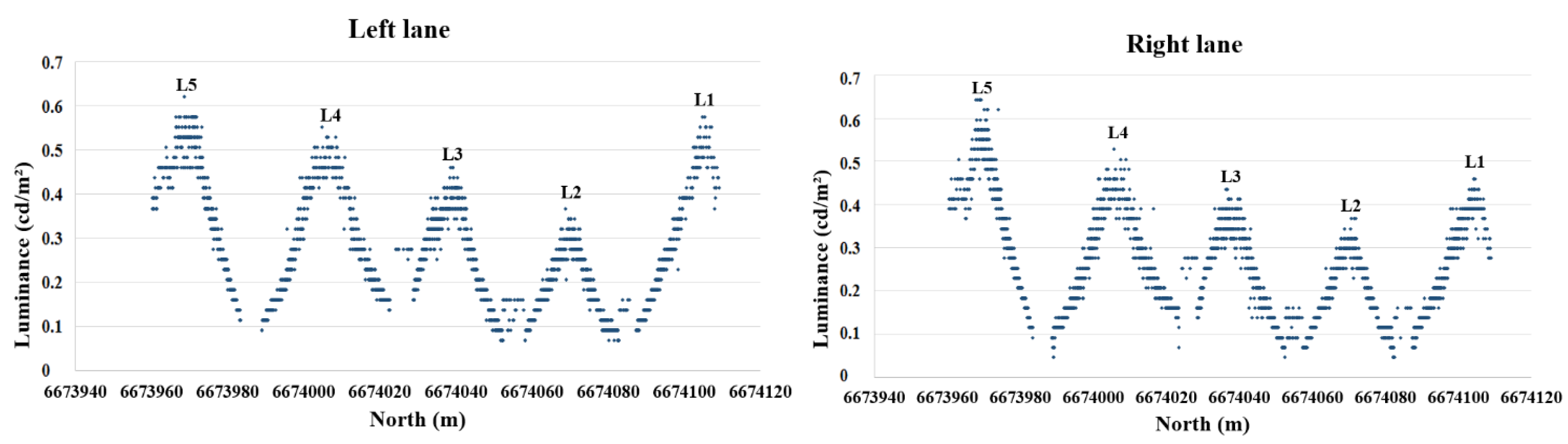
3.2. Statistical Analysis of Road Surface Luminance

The generated 3D luminance data enables us to evaluate the values according to their position or location on the road. Figure 6 shows the scatter plot of the right and left lane luminance values in the longitudinal direction along the centerline of each lane. The luminance values were sampled by calculating an average value for 10 × 10 cm areas for creating the scatter plots in Figure 6 and Figure 7.

Figure 7 shows the scatter plot for comparison between the right and left lane luminance values captured from different directions (positions 3 and 4). The right and left lane samples cover a 20 × 0.1 m area next to the lamp pole and in the middle of the lane. The results show equal luminance values for different capturing directions and they confirm the diffuse reflection behavior of the studied road. We found the standard deviation for the right lane observations to be 0.029 cd/m² and for the left lane 0.036 cd/m².

Figure 6. The (left) and (right) lane luminance values in the longitudinal direction along the centreline of each lane. The position of the lamps (L1–L5) are marked above the corresponding luminance peaks.

Figure 6. The (left) and (right) lane luminance values in the longitudinal direction along the centreline of each lane. The position of the lamps (L1–L5) are marked above the corresponding luminance peaks.

Figure 7. The (left) and (right) lane luminance values in the longitudinal direction along the centreline of each lane. The scatter plot shows the values captured from different directions (position 3, P3; and position 4, P4). The position of the lamp pole and samples are marked in red and blue. Coordinates are presented in ETRS-TM35FIN.

Figure 7. The (left) and (right) lane luminance values in the longitudinal direction along the centreline of each lane. The scatter plot shows the values captured from different directions (position 3, P3; and position 4, P4). The position of the lamp pole and samples are marked in red and blue. Coordinates are presented in ETRS-TM35FIN.

Further, the measured road surface luminances are presented in Table 1. The road surface next to lamp poles was measured with TLS and luminance imaging from both directions of the road as shown in Figure 7. Table 1 compares the results from northerly and southerly directions. Before comparison, the luminance values were sampled by calculating an average value for 10 × 10 cm areas. We derived Average luminance (L_m), Overall Uniformity of luminance (U_o), and Longitudinal Uniformity (U_l) values for three different sections of the road next to lamp poles 2, 3, and 4 [33]. L_m is the average luminance of the carriageway measured at the center of each lane; U_o is the ratio of minimum to average luminance in the defined road area, and U_l refers to the ratio of minimum to maximum luminance in the longitudinal direction along the centerline of each lane. In Table 1 L_m and U_l value is calculated from a 20 × 0.1 m area next to the lamp pole. U_o value is calculated from a 20 × 2.0 m area next to the lamp pole.

Table 1. The comparison of the road surface luminance measured from northerly and southerly directions (N and S). Average luminance (L_m), Overall Uniformity of luminance (U_o), and Longitudinal Uniformity (U_l) values were derived for three different sections of the road next to lamp poles 2, 3, and 4. L_m and U_l are calculated separately for the left and right lane.

Lamp	Direction (/Position)	Lm, Left Lane (cd/m2)	Lm, Right Lane (cd/m2)	Uo (%)	Ul, Left Lane (%)	Ul, Right Lane (%)
L2	N (P1)	0.211	0.221	0.425	0.286	0.267
	S (P2)	0.206	0.214	0.433	0.385	0.286
L3	N (P2)	0.316	0.307	0.446	0.368	0.389
	S (P3)	0.298	0.280	0.396	0.389	0.353
L4	N (P3)	0.383	0.369	0.495	0.478	0.500
	S (P4)	0.346	0.346	0.399	0.318	0.364

Table 1. The comparison of the road surface luminance measured from northerly and southerly directions (N and S). Average luminance (L_m), Overall Uniformity of luminance (U_o), and Longitudinal Uniformity (U_l) values were derived for three different sections of the road next to lamp poles 2, 3, and 4. L_m and U_l are calculated separately for the left and right lane.

Lamp	Direction (/Position)	Lm, Left Lane (cd/m2)	Lm, Right Lane (cd/m2)	Uo (%)	Ul, Left Lane (%)	Ul, Right Lane (%)
L2	N (P1)	0.211	0.221	0.425	0.286	0.267
	S (P2)	0.206	0.214	0.433	0.385	0.286
L3	N (P2)	0.316	0.307	0.446	0.368	0.389
	S (P3)	0.298	0.280	0.396	0.389	0.353
L4	N (P3)	0.383	0.369	0.495	0.478	0.500
	S (P4)	0.346	0.346	0.399	0.318	0.364

4. Discussion

The integration of TLS and luminance imaging in this study proved to be a useful method for creating luminance-corrected 3D point cloud data for evaluating night-time road lighting conditions. In other words, the presented method combines calibrated luminance values (cd/m²) with 3D points. In other studies, the term “luminance correction” has also been connected with a point cloud rendering approach which removes luminance inconsistencies caused by different lighting conditions when taking the various 3D scans with color information [34].

The presented method requires that the relative orientation between the luminance images and intensity images of the 3D point cloud is solved in order to integrate the data sets into the same coordinate system. The registration error for all image pairs was 4.7 pixels, which was mainly caused by lower resolution on TLS intensity images. The calculation of the luminance was based on the RGB output values of a Nikon D800E digital still camera. The camera was calibrated with a reference luminance source. In terms of luminance imaging, it should be noted that the intensity of the reflected light may vary according to the viewing direction, particularly if the road surface is wet. We confirmed the diffuse reflection of the studied road by comparing the luminance values captured from different directions, and we achieved relevant results when the imaging was performed from a driver’s point of view (Figure 7). The standard deviations of the comparison were 0.029 cd/m² and 0.036 cd/m². In this study, we focused on measuring the lighting conditions on the road surface. However, the method can also be used to evaluate the glare in the surrounding area. Luminance-corrected 3D point cloud could also be combined with eye-tracking data [4]. A detailed 3D point cloud produced by TLS also allows for the detection of the shadowing objects, poles, pole orientations, traffic signs, road markings, information boards, and other objects along the road. The results also confirmed that the method can be used to distinguish the variation in the lighting conditions on different sections of the road (Figure 6). Hence, the method is a new tool for monitoring lighting performance and variations of visibility level along the road (see e.g., [35]). In addition, road lighting standards set requirements for maintained average luminance and its uniformity [33]. These values have been calculated in Table 1.

The TLS method requires that the road is closed while the measurements are being taken. In this study, the TLS and image data acquisition from one measurement station took around 10 min; this limits the size of the study area to be examined. This constraint can be avoided by integrating luminance imaging with mobile laser scanning (MLS). This technology is a novel method for collecting street or road inventory data for design, maintenance, rehabilitation, and environment purposes. The MLS method has the ability to identify objects and areas that are difficult and time-consuming to identify via other mapping methods. The benefits of MLS are apparent in a measuring rate context, especially when compared to the TLS method. A good and recent comparison of performance of MLS systems on the market has been made by Kaartinen et al. [36]. In this study, the ROAMER system is compared with commercial systems from Riegl (Riegl VMX-250), Optech (Optech Lynx Mobile Mapper), and Streetmapper 360. In tests performed in a real life situation in the Espoonlahti area, the systems could reach an elevation accuracy of 35 mm from a range of 35 m, with the best system being capable of a planimetric accuracy of 25 mm from a range of 45 m [36]. When integrated to MLS system, the luminance mapping of roads could be performed parallel to MLS road inventories. The requirement for systems capable of measuring road lighting of long road segments, and producing georeferenced data has been brought up in research literature [6,37]. Integration of MLS and luminance measurement could also be applied for this purpose. In addition, other analyses concerning the road environment could be performed from the same data set, as mentioned above.

In this study, the photopic transformation function, presented in Equation (2), was used to calculate luminance values from an RGB image. Related to this, there are two main types of photoreceptor cell in the human eye: cone cells and rod cells. Cone cells are used when there is plenty of light. They are located in the fovea—the central area of the retina—and they make acute color vision possible. Rod cells are specialized in dark vision and are unable to distinguish between colors. Vision where only cone cells are used is called photopic vision, whereas in scotopic vision, only rod cells are used. In mesopic vision, both cone and rod cells are used simultaneously. It is debatable how well the photopic transformation function presented in Equation (2) actually performs. The actual transformation function is different in each digital camera and may differ more or less from the IEC standard [32]. For low scotopic luminance values (<0.005 cd/m²), the transformation function is also different and individual for each digital camera. In addition, if both photopic and scotopic transfer functions are known, it is possible to obtain the mesopic luminance value using the iterative formula presented in CIE 191 [38]. This complex extension was beyond the scope of this study but it could be considered in the future.

5. Conclusions

A promising and novel 3D luminance evaluation approach of night-time road lighting conditions based on luminance-corrected 3D point clouds is demonstrated in this paper. Despite developments in laser scanning technology and applications, we have not found any other studies that have implemented the fusion of laser scanning and luminance imaging data and created luminance-corrected 3D point cloud data. A detailed road environment model with luminance values is obtained using terrestrial laser scanning and luminance imaging with a Nikon D800E camera. The luminance values of the RGB images were calibrated with a reference luminance source, and the calibration showed a linear ratio between the digital values of the Nikon D800E camera and the reference luminance. We integrated these terrestrial data sources in the same coordinate system by determining the orientation of undistorted RGB images relative to the intensity images of individual terrestrial laser scans. In the achieved 3D point cloud every measurement point had also its own calibrated luminance value in addition to coordinates. We assume that in the future, road lighting conditions can also be evaluated by integrating luminance imaging with mobile laser scanning, which improves the measurement rates and increases cost effectiveness.

References

1. Kostic, M.; Djokic, L. Recommendations for energy efficient and visually acceptable street lighting. Energy 2009, 34, 1565–1572. [Google Scholar] [CrossRef]
2. EC 245/2009. COMMISSION REGULATION (EC) No 245/2009 of 18 March 2009 implementing Directive 2005/32/EC of the European Parliament and of the Council with regard to ecodesign requirements for fluorescent lamps without integrated ballast, for high intensity discharge lamps, and for ballasts and luminaires able to operate such lamps, and repealing Directive 2000/55/EC of the European Parliament and of the Council. Available online: http://eur-lex.europa.eu/LexUriServ/LexUriServ.do?uri=OJ:L:2009:076:0017:0044:en:PDF (accessed on 2 September 2015).
3. Kostic, M.; Djokic, L.; Pojatar, D.; Strbac-Hadzibegovic, N. Technical and economic analysis of road lighting solutions based on mesopic vision. Build. Environ. 2009, 44, 66–75. [Google Scholar] [CrossRef]
4. Cengiz, C.; Kotkanen, H.; Puolakka, M.; Lappi, O.; Lehtonen, E.; Halonen, L.; Summala, H. Combined eye-tracking and luminance measurements while driving on a rural road: Towards determining mesopic adaptation luminance. Light. Res. Technol. 2013. [Google Scholar] [CrossRef]
5. Ekrias, A.; Eloholma, M.; Halonen, L.; Song, X.J.; Zhang, X.; Wen, Y. Road lighting and headlights: Luminance measurements and automobile lighting simulations. Build. Environ. 2008, 43, 530–536. [Google Scholar] [CrossRef]
6. Zhou, H.; Pirinccioglu, F.; Hsu, P. A new roadway lighting measurement system. Transp. Res. Part C Emerg. Technol. 2009, 17, 274–284. [Google Scholar] [CrossRef]
7. Manandhar, D.; Shibasaki, R. Auto-extraction of urban features from vehicle-borne laser data. Int. Arch. Photogramm. Remote Sens. Spat. Inf. Sci. 2012, 34, 650–655. [Google Scholar]
8. Jochem, A.; Höfle, B.; Rutzinger, M. Extraction of vertical walls from mobile laser scanning data for solar potential assessment. Remote Sens. 2011, 3, 650–667. [Google Scholar] [CrossRef]
9. Jaakkola, A.; Hyyppä, J.; Hyyppä, H.; Kukko, A. Retrieval algorithms for road surface modelling using Laser-based mobile mapping. Sensors 2008, 8, 5238–5249. [Google Scholar] [CrossRef]
10. Puente, I.; González-Jorge, H.; Martínez-Sánchez, J.; Arias, P. Automatic detection of road tunnel luminaires using a mobile LiDAR system. Measurement 2014, 47, 569–575. [Google Scholar] [CrossRef]
11. Lehtomäki, M.; Jaakkola, A.; Hyyppä, J.; Kukko, A.; Kaartinen, H. Detection of vertical pole-like objects in a road environment using vehicle-based laser scanning data. Remote Sens. 2010, 2, 641–664. [Google Scholar] [CrossRef]
12. Rutzinger, M.; Pratihast, A.K.; Elberink, S.O.; Vosselman, G. Detection and modeling of 3D trees from mobile laser scanning data. Int. Arch. Photogramm. Remote Sens. Spat. Inf. Sci. 2010, 38, 520–525. [Google Scholar]
13. Yang, B.; Wei, Z.; Li, Q.; Li, J. Automated extraction of street-scene objects from mobile Lidar point clouds. Int. J. Remote Sens. 2012, 33, 5839–5861. [Google Scholar] [CrossRef]
14. Arastounia, M.; Elberink, S.O.; Khoshelham, K.; Diaz Benito, D. Rail track detection and modeling in mobile laser scanner data. ISPRS Ann. Photogram. Remote Sens. Spat. Inform. Sci. 2013, 5, 223–228. [Google Scholar]
15. Wu, B.; Yu, B.; Yue, W.; Shu, S.; Tan, W.; Hu, C.; Huang, Y.; Wu, J.; Liu, H. A voxel-based method for automated identification and morphological parameters estimation of individual street trees from mobile laser scanning data. Remote Sens. 2013, 5, 584–611. [Google Scholar] [CrossRef]
16. Rönnholm, P.; Honkavaara, E.; Litkey, P.; Hyyppä, H.; Hyyppä, J. Integration of laser scanning and photogrammetry (Key-note). Int. Arch. Photogramm. Remote Sens. Spat. Inf. Sci. 2007, 36, 355–362. [Google Scholar]
17. Alba, M.I.; Barazzetti, L.; Scaioni, M.; Rosina, E.; Previtali, M. Mapping infrared data on terrestrial laser scanning 3D models of buildings. Remote Sens. 2011, 3, 1847–1870. [Google Scholar] [CrossRef]
18. González-Aguilera, D.; Rodriguez-Gonzalvez, P.; Armesto, J.; Lagüela, S. Novel approach to 3D thermography and energy efficiency evaluation. Energy Build. 2012, 54, 436–443. [Google Scholar] [CrossRef]
19. Lubowiecka, I.; Arias, P.; Riveiro, B.; Solla, M. Multidisciplinary approach to the assessment of historic structures based on the case of a masonry bridge in Galicia (Spain). Comput. Struct. 2011, 89, 1615–1627. [Google Scholar] [CrossRef]
20. Zhu, L.; Hyyppä, J.; Kukko, A.; Jaakkola, A.; Lehtomäki, M.; Kaartinen, H.; Chen, R.; Pei, L.; Chen, Y.; Hyyppä, H.; Rönnholm, P.; Haggren, H. 3D city model for mobile phone using MMS data. In Proceedings of the Urban Remote Sensing Joint Event, Shanghai, China, 20–22 May 2009.
21. Alamús, R.; Kornus, W. DMC geometry analysis and virtual image characterisation. Photogramm. Record 2008, 23, 353–371. [Google Scholar] [CrossRef]
22. Brenner, C.; Haala, N. Rapid acquisition of virtual reality city models from multiple data sources. Int. Arch. Photogramm. Remot. Sens. 1998, 32, 323–330. [Google Scholar]
23. Virtanen, J.-P.; Puustinen, T.; Pennanen, K.; Vaaja, M.T.; Kurkela, M.; Viitanen, K.; Rönnholm, P. Customized visualizations of urban infill development scenarios for local stakeholders. J. Build. Constr. Plan. Res. 2015, 3, 68–81. [Google Scholar] [CrossRef]
24. Kanzok, T.; Linsen, L.; Rosenthal, P. An interactive visualization system for huge architectural Laser Scans. In Proceedings of the 10th International Conference on Computer Graphics Theory and Applications, Berlin, Germany, 11–14 March 2015; pp. 265–273.
25. Chow, J.; Lichti, D.; Teskey, W. Accuracy assessment of the Faro Focus3D and Leica HDS6100 panoramic type terrestrial laser scanner through point-based and plane-based user self-calibration. In Proceedings of the FIG Working Week: Knowing to Manage the Territory, Protect the Environment, Evaluate the Cultural Heritage, Rome, Italy, 6–10 May 2012.
26. Meyer, J.E.; Gibbons, R.B.; Edvards, C.J. Development and Validation of a Luminance Camera, Final Report; Virginia Tech Transportation Institute: Blacksburg, VA, USA, 2009. [Google Scholar]
27. Wüller, D.; Gabele, H. The usage of digital cameras as luminance meters. Proc. SPIE 2007. [Google Scholar] [CrossRef]
28. Hiscocks, P.D.; Eng, P. Measuring Luminance with a Digital Camera: Case History. Available online: http://www.ee.ryerson.ca:8080/~phiscock/astronomy/light-pollution/luminance-case-history.pdf (accessed on 2 September 2015).
29. Fryer, J.G.; Brown, D.C. Lens distortion for close-range photogrammetry. Photogramm. Eng. Remote Sens. 1986, 52, 51–58. [Google Scholar]
30. CIE 1932. In Commission Internationale de l'Eclairage Proceedings; Cambridge University Press: Cambridge, UK, 1931.
31. CIE 1926. In Commission Internationale de l'Eclairage Proceedings; Cambridge University Press: Cambridge, UK, 1924.
32. IEC 61966-2-1. In Multimedia Systems and Equipment—Colour Measurements and Management—Part 2-1: Colour Management—Default RGB Color Space—sRGB; International Electrotechnical Commission: Geneva, Switzerland, 1999.
33. EN 13201. European Standard EN 13201-2. Road lighting. Part 2: Performance Requirements. Available online: https://www.fer.unizg.hr/_download/repository/en_13201-2_.pdf (accessed on 2 September 2015).
34. Kanzok, T.; Linsen, L.; Rosenthal, P. On-the-fly luminance correction for rendering of inconsistently lit point clouds. J. WSCG 2012, 20, 161–169. [Google Scholar]
35. Güler, Ö.; Onaygil, S. The effect of luminance uniformity on visibility level in road lighting. Light. Res. Technol. 2003, 35, 199–213. [Google Scholar] [CrossRef]
36. Kaartinen, H.; Hyyppä, J.; Kukko, A.; Jaakkola, A.; Hyyppä, H. Benchmarking the performance of mobile laser scanning systems using a permanent test field. Sensors 2012, 12, 12814–12835. [Google Scholar] [CrossRef]
37. Cai, H.; Li, L. Measuring light and geometry data of roadway environments with a camera. J. Transp. Technol. 2014, 4, 44–62. [Google Scholar] [CrossRef]
38. Commission Internationale de l’Eclairage. Recommended System for Mesopic Photometry Based on Visual Performance; CIE Publication 191: Vienna, Austria, 2010; p. 79. [Google Scholar]