1. Introduction
Agriculture monitoring systems are valuable decision making tools for forecasting production [
1] and assessing the impacts on food production of threats like droughts [
2], floods [
3], diseases [
4] or civilian conflicts [
5]. In this regard, satellite remote sensing is a critical source of data for these systems, as it offers timeliness, global coverage and objective observation [
6,
7,
8].
At least two types of information are crucial in the delivery of crop production information for any given year: cropland areas and yield estimation or the yield indicator [
9]. The latter can be derived from crop growth condition or status (plant stress, crop damage or vegetation condition, using, for example, NDVI or fAPAR). Moreover, the timeliness of information delivery is key. The earlier the estimation (ideally before the harvest), the more efficient the management and political responses [
10]. To meet these agriculture monitoring requirements, remote sensing research has focused on yield estimation [
11,
12], soil moisture estimation [
13], biophysical variable retrieval [
14] and cropland, or crop type, classification [
15,
16,
17].
A large range of cropland mapping strategies, operating on different scales and associated with varying levels of accuracy, can be found in the literature. On the one hand, annual cropland mapping in the USA [
18] or in Canada [
19] is operational through the use of early
in situ information that mainly comes from field campaigns or from farmers’ declarations. On the other, most studies tackle cropland mapping at a local level, with one or several methodologies often relying on a single sensor. This leads to a large number of local or regional monitoring capabilities, but very few global agricultural mapping experiences [
20,
21]. Moreover, examples of multi-site assessments, which compare the performances of the same classification method in different agrosystems are very scarce. The launch of Sentinel-2, with its swath of 290 km, calls for the development of methods capable of covering large areas and of being transferable from one agricultural region to another. From this perspective, the SPOT 4 Take 5 experiment provides a unique time-series of spatial and temporal resolution similar to that produced by Sentinel-2. This enables us to face the challenges raised by the multi-sites approach, such as
in situ data dependence, common standard definition and methodological improvements.
The term “cropland” has not as yet been clearly defined in the literature. For instance, the U.S. Department of Agriculture (USDA) includes in its cropland definition “all areas used for the production of adapted crops for harvest”, which covers both cultivated and non-cultivated areas [
22]. In most global land cover products, such as GLC2000 [
23], GlobCover 2005/2009 [
24,
25], GLCShare [
26], MODIS Land Cover [
27] and as recently documented in [
28], croplands are partly combined in mosaic or mixed classes (variously including meadows and pastures), making them difficult to use in agricultural applications, either as agricultural masks or as a source for area estimates. Even the most recent and more precise ESA Climate Change Initiative (CCI) Land Cover products, obtained from a multi-year multi-sensor approach, still consider croplands as any other land cover class [
25]. Within the framework of GEO Global Agricultural Monitoring (GEOGLAM) [
29,
30], the Joint Experiment of Crop Assessment and Monitoring (JECAM) [
31] initiative develops a convergence of standards for monitoring and reporting protocols, as well as best practice documents for a variety of remote sensing activities. Based on the FAO study’s uses of the Land Cover Meta Language [
32], the cropland class, defined by JECAM and adopted for this study, consists of “
a piece of land of minimum 0.25 ha (min. width 30 m) that is sowed/planted and harvestable at least once within the 12 months after the sowing/planting date. The annual cropland produces an herbaceous cover and is sometimes combined with some tree or woody vegetation”. There are however three known exceptions to this definition. The first concerns the sugarcane plantation and cassava crop, which are included in the cropland class, although they have a longer vegetation cycle and are not planted yearly. Second, taken individually, small plots, such as legumes, do not meet the minimum size criteria of the cropland definition. However, when considered as a continuous heterogeneous field, they should be included in the cropland. The third case is the greenhouse crops that cannot be monitored by remote sensing and are thus excluded from the definition [
33].
Classification methods for generating cropland maps deal with
in situ or prior knowledge availability. This prior knowledge is required for labeling clusters in unsupervised approaches, as well as for information used to derive inferred function for classifying new data. Managing this site-specific information is key to allowing spatial extension to a multi-site or even a global approach [
34,
35].
Another aspect of the cropland mapping, independent of the classification algorithm, is related to the spatial unit, whether this is the pixel or the object. Pixel-based classifications methods often fail to determine the actual limits of agriculture parcels [
36]. Spatial filters improve the accuracy by removing the small inclusions of other classes within the dominant class [
37]. Parcel-based approaches were found to be more accurate than pixel-based approaches [
15]. Field limits can be derived either from a digital vector database [
38] or by segmentation [
39]. The accuracy of the results is also influenced by the image processing unit (
i.e., the pixel or field). For instance, in landscapes with mixed agriculture and pastoral land cover classes (e.g., Sahelian countries), image segmentation methods seem to provide a considerable advantage, since these land cover types are structurally fairly dissimilar while also being spectrally similar [
40].
The aim of this paper is to propose and demonstrate an automated methodology for annual cropland mapping performing along the season in various agricultural systems using high spatial and temporal resolution remote sensing time series. This research attempts to tackle some of the operational challenges by alleviating the annual
in situ data dependency and by proposing a generic methodology directly applicable in various environments. The methodology includes: (1) an approach leveraging existing high resolution baseline land cover information, if available, or a globally available baseline, if not; (2) an extraction of crop-specific spectral-temporal features targeting the most relevant reflectances to differentiate the cropland; and (3) a flexible and robust classification algorithm. This study corresponds to the development phase of the European Space Agency (ESA) Sentinel-2 for Agriculture (Sen2Agri) project [
41].
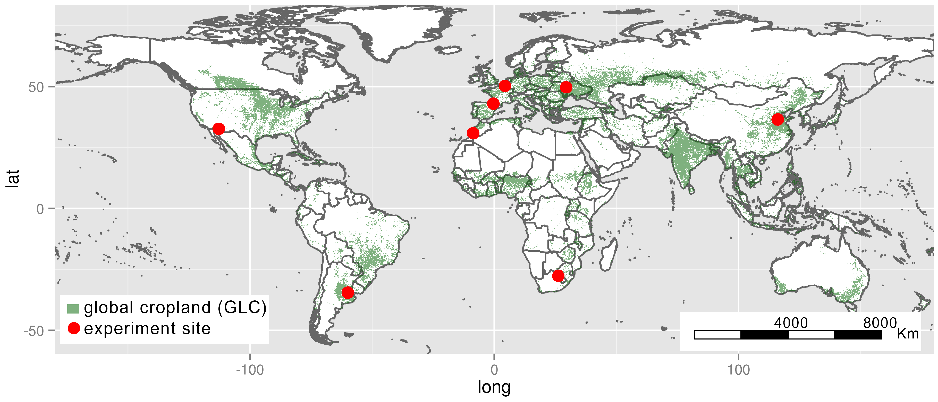
The method is assessed on eight sites with very different agrosystems, which are described below. The core of the paper focuses on the accuracy and performance assessment of the methodology. The impact on the accuracy of the baseline resolution and the spatial unit are also assessed. Finally, the feasibility of implementing the method in a crop monitoring program is discussed, and the paper concludes with an evaluation of its prospects as a generic cropland mapping approach.
3. Methodology
The methodology was designed to exploit time series covering large areas with very different agricultural landscapes and without in situ observations. This cropland mapping approach was tested on the eight sites combining two different classification algorithms and two types of spatial unit, i.e., the pixel versus the object-based approach.
3.1. Building Baseline Land Cover Information
Already existing land cover information was used to build the baseline, required as prior classification knowledge. This land cover information consisted of existing (and some possibly out-dated) land cover maps, which were at high spatial resolution (20 m). Where no high resolution land cover map was available, medium resolution (300 m) global land cover information served as the baseline. For instance, in France and Belgium, the data extracted from the LPIS were merged with the global ESA CCI Land Cover with priority given to the LPIS on overlapping areas (
Table 4 [
25,
43,
44,
45,
46,
47]). Since existing maps were potentially outdated because of changes that may have occurred since the map was produced, it was necessary to include a cleaning process in our methodology to remove this misleading information. This cleaning process also reduced possible mapping error in the pre-existing maps.
3.2. Crop-Specific Temporal Features
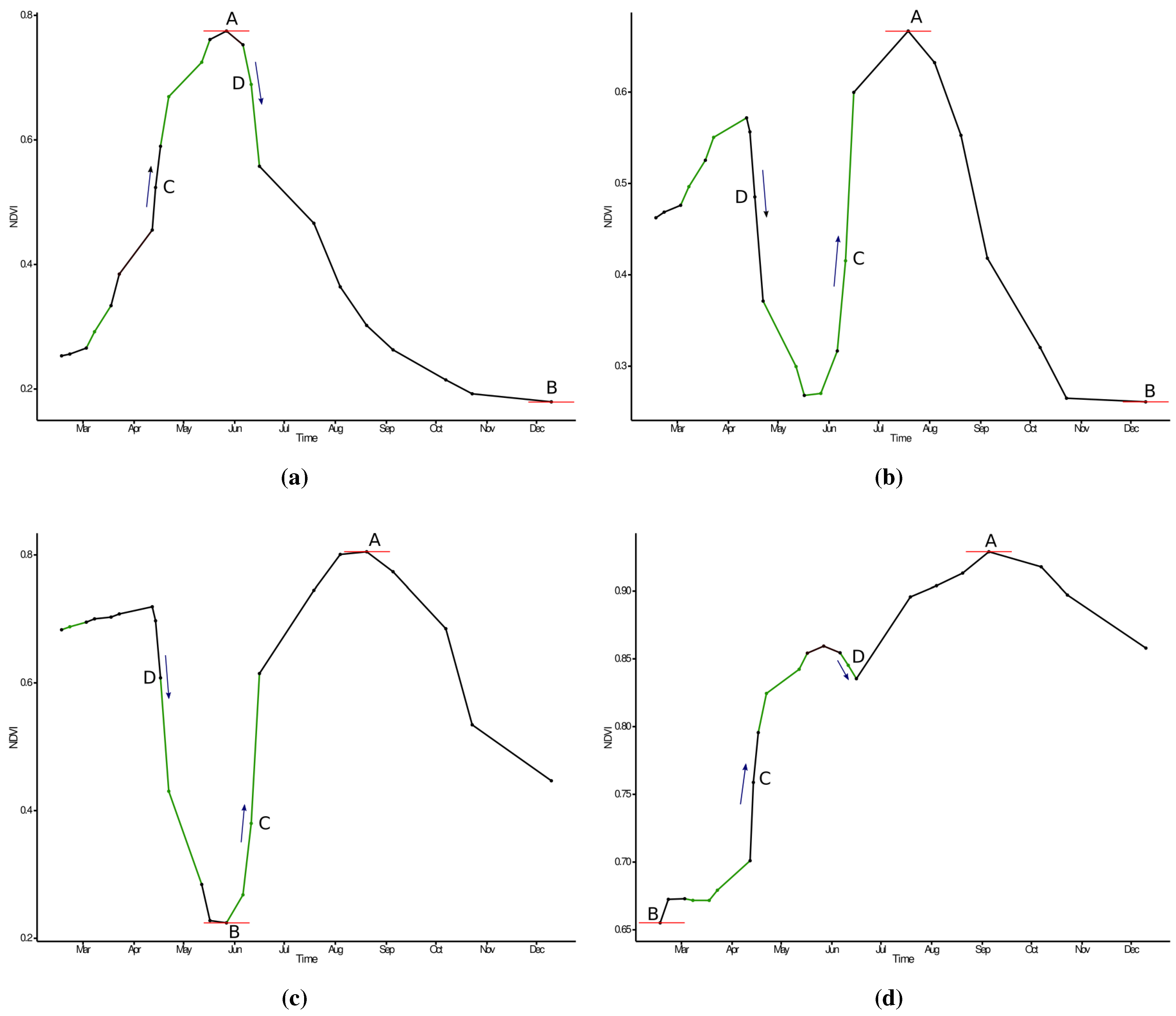
The second step in the methodology was to identify and extract relevant spectral and temporal features to differentiate the cropland from the other land cover types. These features were defined according to generic characteristics of crop growth. Typically, the crop development cycle [
48] can be characterized by four key elements: (1) the growing of crops on bare soil after tillage and sowing; (2) a higher growing rate than natural vegetation types; (3) a well-marked peak of green vegetation; and (4) a fast reduction of green vegetation due to harvest and/or senescence (
Figure 3).
Table 4.
Respective mapping source to build the baseline land cover information. This baseline serves as input for the classification. LPIS, Land Parcel Identification System; CCI, Climate Change Initiative.
Table 4.
Respective mapping source to build the baseline land cover information. This baseline serves as input for the classification. LPIS, Land Parcel Identification System; CCI, Climate Change Initiative.
| Site | Information Used in the Baseline |
|---|
| Belgium | Belgian LPIS (20 m) (2012) [43], CCI Land Cover (300 m) [25] |
| Argentina | Global land cover GLC30 (30 m) [44] |
| China | Global land cover GLC30 (30 m) [44] |
| France | French LPIS (2012) (20 m) [43], CCI Land Cover (30 m) [25] |
| Morocco | CCI Land Cover (300 m) [25] |
| South Africa | Water bodies SRTM-SWBD(30 m) [45], SADCLand Cover Dataset (30 m) (2000) [46], CCI Land Cover (300 m) [25] |
| Ukraine | Classification map (30 m) provided by JECAM site manager (2010) |
| USA | USDA data layer 2012 (20 m) [47] |
Based on this conceptual framework, five distinct remote sensing stages in the crop cycle could be defined at the pixel scale: (1) the maximum value of red; (2) the maximum positive slope of the NDVI time series; (3) the maximum value of NDVI; (4) the maximum negative slope of the NDVI time series; and (5) the minimum value of NDVI. The final spectral-temporal features corresponded to the reflectance values observed at these stages. These features were time independent, which allowed us to deal with the cropland diversity and the agro-climatic gradient across the landscape.
Twenty features (four spectral bands of the five crop growth characteristics) are too numerous as input for most of the classifiers, as this can lead to a performance deterioration due to Hughes’ phenomenon [
49]. Specific feature combinations were selected in order to create a relevant set of features for differentiating croplands from non-cropland. Following a preselection step, it was found that the SWIR band did not provide valuable enough information, and it was discarded. The final features were selected as the set of five features providing the best mean overall accuracy (OA) on all of the test sites. This included the red and NIR reflectances from the minimum NDVI stage and the green, red and NIR from the maximum NDVI stage.
3.3. Classification Algorithms
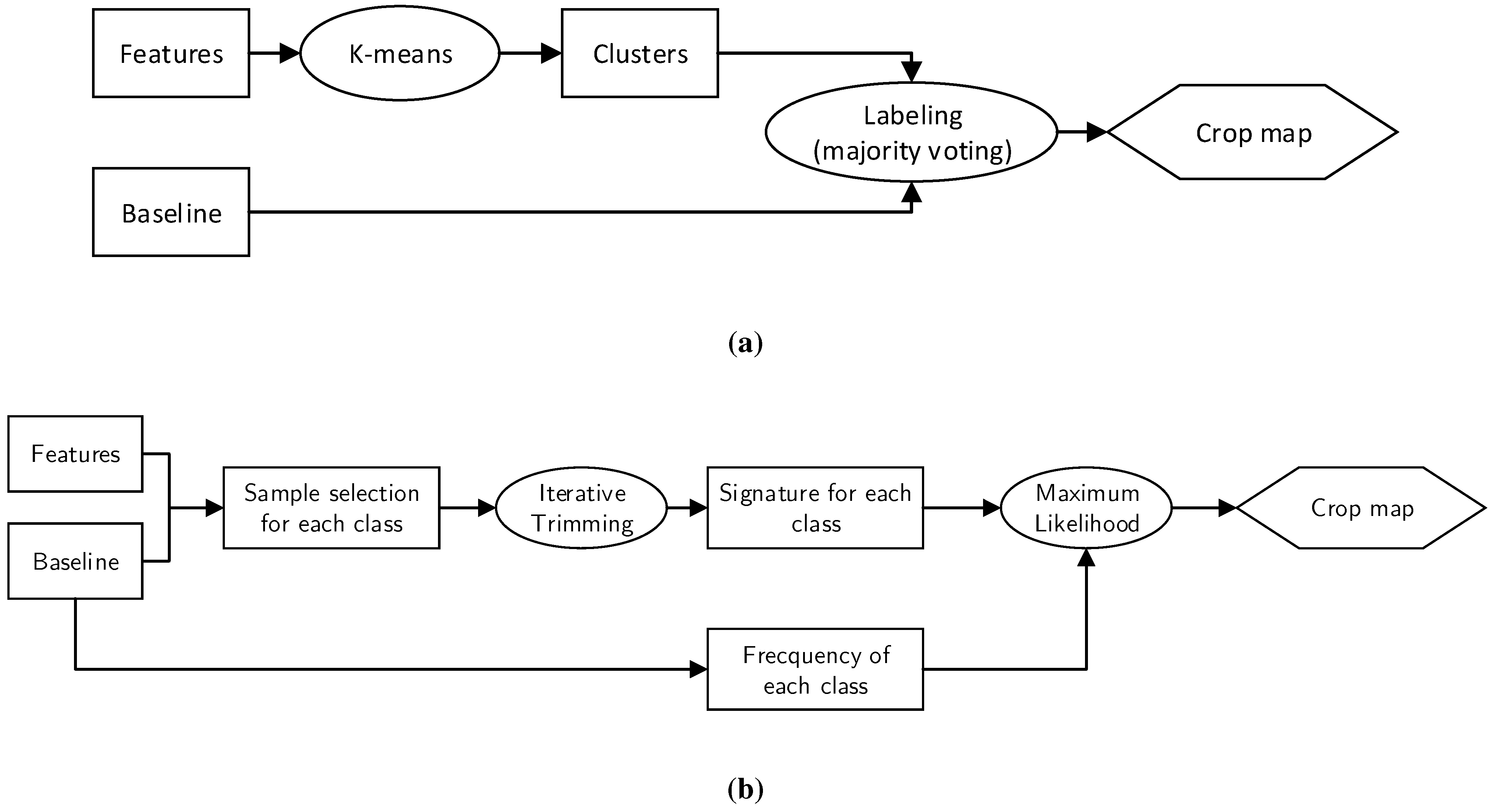
To classify the remote sensing features, two different algorithms were compared (
Figure 4). The first was the K-means, an unsupervised classifier commonly found in the literature [
50], followed by an automated labeling of the clusters (
Figure 4). K-means clustering consisted of minimizing the mean square
d-dimensional distance between each pixel to its closest cluster center [
51]. One hundred clusters were created, aggregating spectrally-close pixels. The baseline was used for labeling the clusters, based on a simple majority-voting rule, which consisted of labeling clusters as cropland if more than half of the cluster pixels corresponded to the cropland class of the baseline. If not, the cluster is labeled as non-cropland.
Figure 3.
Temporal NDVI profile for crop surfaces (a,b), grassland surface (c) and forest (d), all located in France with dates where interpolated reflectances were used to compute the NDVI (green dots and lines) and temporal features (A: maximum value of NDVI; B: minimum value of NDVI; C: maximum slope; D: minimum slope).
The second algorithm, the trimming method, was a two-step, supervised classification. First, a cleaning process removed any pixels likely to have been mislabeled from the baseline by iterative trimming, and second, a maximum likelihood classifier was applied.
The iterative trimming step consisted of removing from a given frequency distribution the least probable values that behave like outliers [
52,
53]. The purpose of this procedure was to reduce the sensitivity to outliers of parameter estimates, such as the sample mean and variance. For each class, the selection of outliers relied on a probability threshold
α, which specified the limit at which an observation was considered to be an outlier. As the estimates of the distribution parameters were influenced by the outliers, the trimming was iteratively performed until no more outliers were identified.
As we assumed a Gaussian distribution of reflectances for any given class, outliers were defined as values that were outside the commonly-agreed interval, described by the distribution variance:
where
was the upper (100
α)-th percentile of a
distribution with
p degrees of freedom. Outliers were mainly due to recent land cover changes and the discrepancy between the existing land cover information and the EO dataset, often due to spatial resolution mismatches (20 m
versus up to 300 m for the land cover maps). A sample of 1000 pixels, randomly selected for each class of the baseline, provided the distribution of the spectral signature of this class, which was then cleaned by iterative trimming with a threshold
α of 0.01. This resulted in a more robust spectral signature for each class, defined by the legend of the baseline. These different spectral signatures were then used in a conventional maximum likelihood classifier [
54,
55]. Finally, a translation of the cropland and non-cropland classes as defined by the baseline legend yielded the final cropland map.
Figure 4.
Flow charts for both algorithms describing the main classification steps. Boxes correspond to data (input/output); ellipses correspond to processing steps; and diamonds correspond to final results.(a) The K-means-based approach is made up of a first step of clustering followed by majority-voting cluster labeling. (b) The trimming-based approach is made up of a first step of baseline cleaning (iterative trimming) followed by a maximum likelihood classifying process to produce the final result.)
3.4. Baseline Resolution Impact Assessment
The spatial resolution of the land cover baseline that was used as input ranged from 20 m in Belgium to 300 m in Morocco. The impact of this resolution difference was assessed by comparing the results obtained from a global baseline instead of the more precise local one. This assessment allowed us to test the methodology’s robustness when a global land cover was the only source available and, thus, the possibility of applying the methodology on a larger scale. Moreover, the influence of the baseline accuracy was also assessed by systematically adding noise to the baseline and observing the impact on classification results. The noise consisted of a random class permutation of a given percentage of the total pixels, which ranged from 0%–70%. Obviously, only sites where a local high resolution baseline was available were tested (i.e., Belgium, France, South Africa, Ukraine and the USA).
3.5. Spatial Unit Assessment
Two different spatial units were considered,
i.e., the pixel and the object. The objects resulted from a segmentation step based on the mean-shift segmentation algorithm. This algorithm was applied to the set of the six first principal components obtained by a principal component analysis (PCA) transformation on the full NDVI times series [
56].
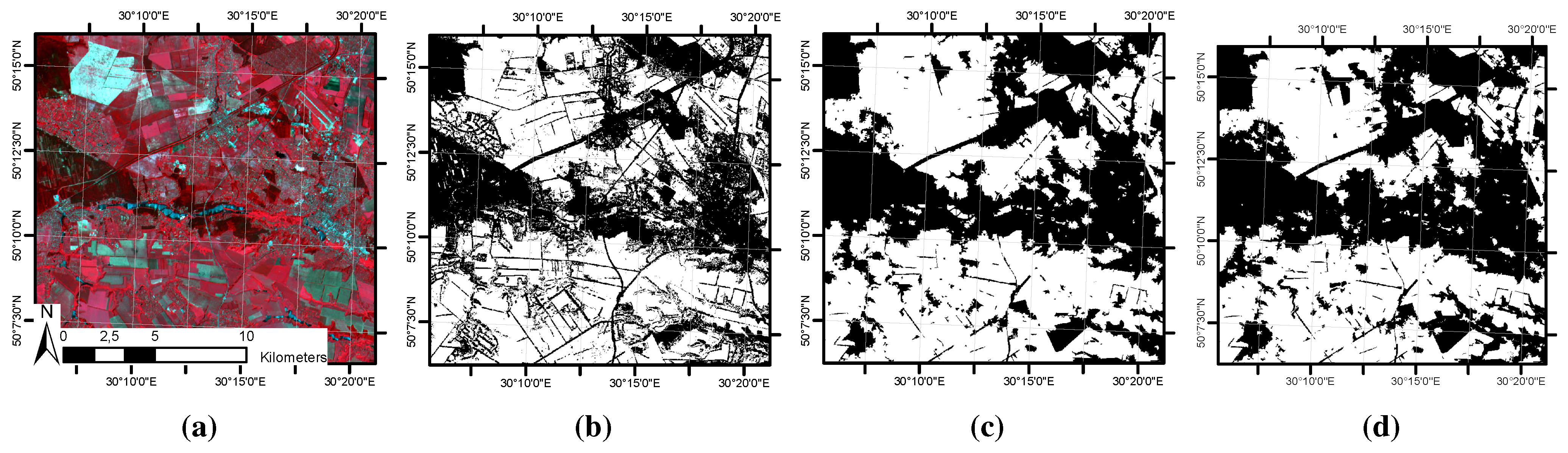
This segmentation reduced the salt and pepper effect that was visible in most of the per pixel classification maps and increased the spatial consistency (
Figure 5). The objects were used in two different ways: first, as a standard object-based classification, applied to a spectral signature averaged at the object level, and, second, as a post-processing step to filter the pixel-based classification result, using a majority-voting rule. The impact of the spatial unit was assessed by comparing the corresponding accuracies using the best performing classification algorithm.
Figure 5.
Spatial unit impact on cropland (in white) mapping. (a) The SPOT 4 image acquired on 11 June 2013. (b) The pixel-based result presents the salt and pepper effect, preventing a sharp field delineation. (c) The object post-filtering approach is a dual approach combining both aspects. (d) The object-based classification result is spatially more consistent.
3.6. Crop Mapping along the Season
It was predicted that the proposed algorithm could be applied in a dynamic system that would produce cropland masks along the season with increased accuracy. The methodology was run repeatedly using the available time series from Month 1 to Month 12 in order to assess its performance along the season.
Four delivery periods were considered for producing maps along the season at three-month intervals. Both the OA and F-scores for each map were assessed using the same validation dataset. The start of the EO time series coincided with the beginning of the growing season for most of the Northern Hemisphere’s sites, although this was not the case for the Southern Hemisphere. The growing cycle ended after three months of the time series, and then, a new growing season was initiated. It was possible that the new information acquired was in some cases different, and consequently, this added noise to the cropland class during the trimming step and some temporal disagreement.
3.7. Performance Assessment
The performance of the different approaches was assessed for timeliness by two complementary criteria, namely the accuracy assessment and across-site robustness. Two different metrics, derived from the confusion matrix, were selected for the OA assessment. The OA evaluated the overall effectiveness of the algorithm, while the F-score measured the accuracy of a class using the precision and recall measures.
The OA was calculated as the total number of correctly-classified pixels divided by the total number of validation pixels:
The precision or user’s accuracy for class
i was the fraction of correctly-categorized pixels with regard to all pixels classified as this class
i in the classification results:
The recall or producer’s accuracy for class
i was the fraction of correctly-classified pixels with regard to all pixels of that ground truth class
i:
The F-score (also known as the F-1 score or F-measure) for class
i was the harmonic mean of the precision and recall and reached its maximum value at 1 and minimum score at 0:
4. Results
The different combinations of classification algorithms (i.e., K-means or a maximum likelihood classifier including a trimming) and spatial units (i.e., either the pixel, the object-based classification or the object-based filtering) were applied on the eight test sites. In addition to the systematic accuracy assessment, the robustness of the input dataset was analyzed with regard to information timeliness and the baseline resolution.
4.1. Crop Mapping Methodologies Assessment
The accuracy of the cropland maps provided by the different methodologies was assessed using independent validation datasets. In general, the approach combining the trimming and the maximum likelihood classifier provided better OA than the K-means approach (
Table 5). This difference ranged from less than 1% (USA) to 12% (Argentina), depending on site characteristics. The K-means approach tended to overestimate the cropland area (
Figure 6). While Ukraine, France and the USA sites showed rather constant results, some of the other results are worth discussing.
The poor quality of the baseline and the limited presence of the non-crop class in Argentina meant that the K-means algorithm was unable to distinguish non-cropland, because all pixels were labeled as cropland. Using the same baseline, the trimming-based method succeeded in distinguishing both classes, thereby increasing the OA by 20%, albeit still with only 30% of recall for non-cropland.
Despite the short duration of the EO time series for Belgium, the accuracy level reached 89% even for the K-means algorithm. This underlines the importance of an appropriate temporal distribution of observation, which can compensate for the low frequency of cloud-free observation for cropland mapping.
In the case of the Chinese site, the OA reached 68% for K-means, while the trimming method yielded an accuracy of 82%, corresponding to an increase of 14%. The main improvement was found in the cropland precision and non-cropland recall pair, showing an overestimation of the cropland area by the K-means (represented by the blue patches in
Figure 6f).
In South Africa, the OA was only slightly improved by using the trimming method as compared to the K-means. It is worth highlighting the non-cropland recall and precision. While the K-means underestimated non-cropland by 78%, it showed good non-cropland precision. Thanks to the cleaning process achieved by the trimming, the omission error was reduced from 78% down to 49% with quite low commission errors. This is illustrated by the blue patterns in
Figure 6b, which correspond to the cropland mapped by the K-means algorithm.
The Moroccan site presented the poorest cropland precision results for both the trimming and the K-means approaches, mainly due to an overestimation of cropland extent. Unlike the other sites, these performances were related to a landscape that was not dominated by cropland. Indeed, non-cropland pixels were 40-times more abundant than cropland pixels. Misclassified cropland pixels, therefore, have no effect on the non-cropland precision results (i.e., false negatives are not able to compensate for the huge amount of true negatives). Finally, cropland precision was also particularly low because the error of cropland overestimation could not really be compensated for by a good cropland classification due to their unbalanced proportions. As such, the recall remained the only reliable indicator for an accuracy assessment for Morocco, and the trimming method performed best for both cropland and non-cropland recalls.
It is also worth mentioning that the three sites with the highest accuracy differences between the two algorithms, i.e., Argentina, China and Morocco, were the sites for which a high resolution baseline was not available. This demonstrates a better ability to deal with coarse land cover baseline when using the trimming approach, yielding generic performances. Because these results demonstrated that trimming outperformed the K-means approach for every site, only the results from the trimming approach will be used in the assessments below.
Table 5.
Accuracy results for the eight sites obtained by the K-means algorithm at the pixel scale (pxl) and the maximum likelihood classifier with the trimming method at the pixel scale (pxl), at the object-level (OB) or filtered by objects (filter).
Table 5.
Accuracy results for the eight sites obtained by the K-means algorithm at the pixel scale (pxl) and the maximum likelihood classifier with the trimming method at the pixel scale (pxl), at the object-level (OB) or filtered by objects (filter).
| | | | Cropland | Non-Cropland |
|---|
| Site | Method | Overall Accuracy | Precision | Recall | Precision | Recall |
|---|
| Argentina | K-means pxl | 59.2 | 59.2 | 100.0 | 0.0 | 0.0 |
| trimming pxl | 71.4 | 67.6 | 99.2 | 96.5 | 30.9 |
| trimming OB | 87.0 | 82.6 | 99.0 | 98.0 | 69.6 |
| trimming filter | 59.1 | 59.2 | 99.8 | 1.9 | 0.0 |
| Belgium | K-means pxl | 88.6 | 87.3 | 96.0 | 91.5 | 75.7 |
| trimming pxl | 89.8 | 89.9 | 94.5 | 89.4 | 81.5 |
| trimming OB | 89.4 | 89.3 | 94.7 | 89.7 | 80.2 |
| trimming filter | 91.5 | 87.4 | 89.4 | 93.9 | 92.6 |
| China | K-means pxl | 68.4 | 46.6 | 96.9 | 98.0 | 57.5 |
| trimming pxl | 82.2 | 61.8 | 93.6 | 96.9 | 77.9 |
| trimming OB | 85.9 | 67.3 | 95.2 | 97.8 | 82.3 |
| trimming filter | 86.1 | 67.7 | 95.3 | 97.9 | 82.6 |
| Ukraine | K-means pxl | 89.4 | 94.3 | 93.7 | 50.9 | 53.6 |
| trimming pxl | 90.5 | 93.1 | 96.6 | 58.9 | 40.7 |
| trimming OB | 91.5 | 93.7 | 97.0 | 65.3 | 46.4 |
| trimming filter | 91.7 | 69.4 | 41.5 | 93.2 | 97.8 |
| South Africa | K-means pxl | 85.6 | 85.4 | 99.5 | 90.1 | 21.8 |
| trimming pxl | 88.8 | 90.1 | 97.0 | 78.4 | 51.0 |
| trimming OB | 90.0 | 93.1 | 94.8 | 74.0 | 67.4 |
| trimming filter | 91.3 | 76.5 | 74.0 | 94.4 | 95.1 |
| France | K-means pxl | 86.3 | 83.4 | 76.7 | 87.7 | 91.6 |
| trimming pxl | 81.5 | 69.2 | 86.2 | 91.2 | 78.9 |
| trimming OB | 72.0 | 56.6 | 90.6 | 92.3 | 61.8 |
| trimming filter | 87.6 | 79.6 | 87.5 | 92.7 | 87.7 |
| Morocco | K-means pxl | 73.3 | 5.4 | 84.8 | 99.6 | 73.1 |
| trimming pxl | 76.4 | 6.8 | 96.0 | 99.9 | 76.1 |
| trimming OB | 81.4 | 8.5 | 95.4 | 99.9 | 81.2 |
| trimming filter | 76.5 | 99.9 | 76.1 | 6.9 | 96.8 |
| USA | K-means pxl | 99.0 | 95.7 | 92.4 | 99.3 | 99.6 |
| trimming pxl | 98.6 | 91.3 | 93.1 | 99.3 | 99.2 |
| trimming OB | 98.6 | 90.1 | 93.9 | 99.4 | 99.0 |
| trimming filter | 99.0 | 99.2 | 99.7 | 96.2 | 91.8 |
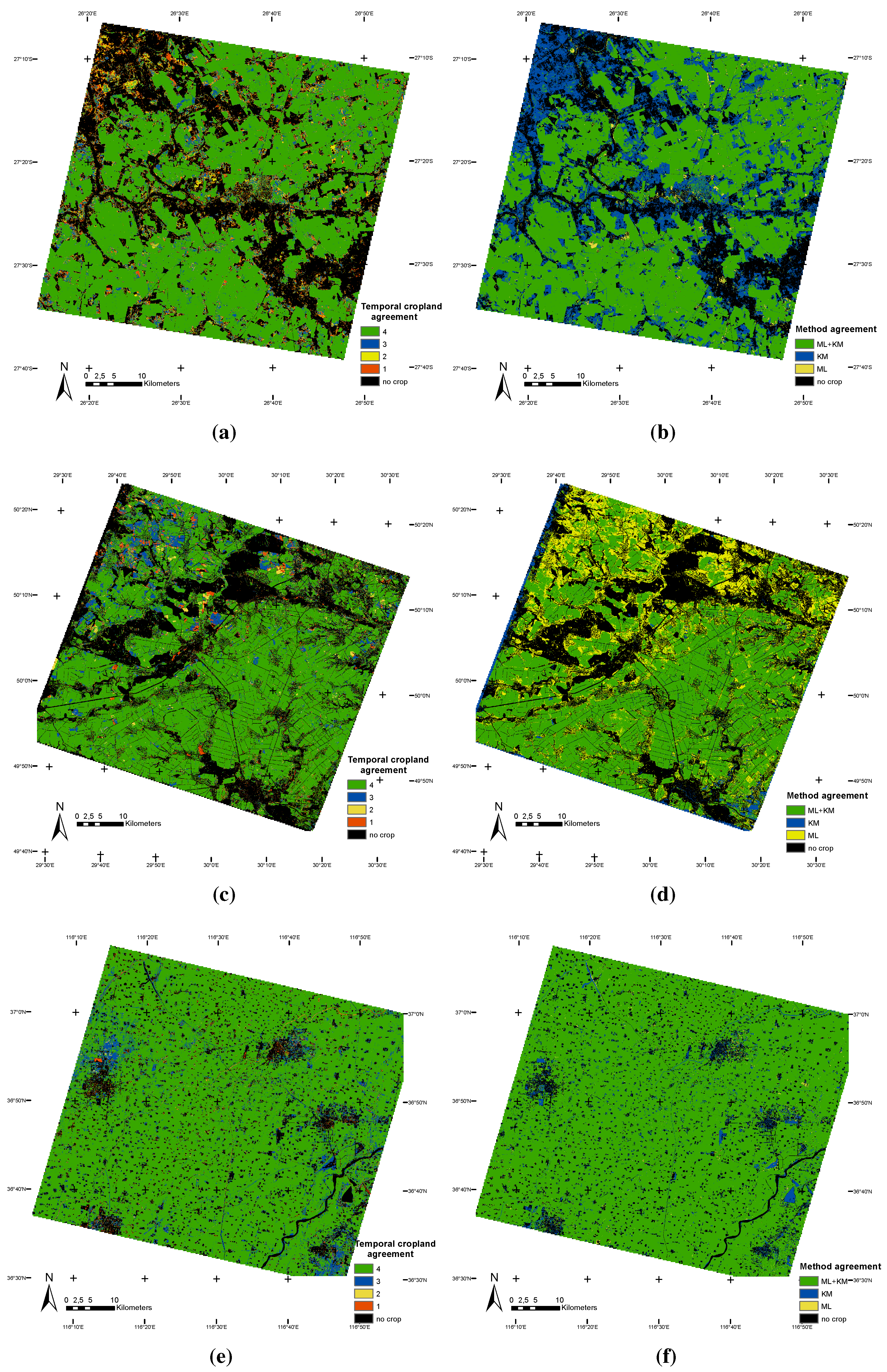
Figure 6.
Temporal comparison (left-hand column), displaying the number of cropland detections along the season respectively after three, six, nine and twelve months. Method comparison (right-hand column) in South Africa (a,b), Ukraine (c,d) and China (e,f) between trimming and K-means (0: non-cropland for both classifications; ML: cropland detected only by the maximum likelihood, preceded by the iterative trimming; KM: cropland only detected by the K-means method; ML + KM: cropland identified by both methods).
4.2. Spatial Unit Assessment
First, the effect of the sites’ characteristics prevailed over the spatial unit effect in most cases, since the OA difference between sites was greater than the OA difference between spatial units for any given site (
Table 5). The exceptions to this were Argentina, France and Morocco, which are discussed further below. Second, the object-based approaches provided rather similar or slightly better performances than the pixel-based approach. However, this slight difference does not really balance out the additional computing cost of the segmentation step.
Only the French site presented a significant decrease in OA (−11%) for the object-based classification and only a slight increase when using objects for post-processing. This difference was mainly due to the specific spatial structure of vineyards, accurately classified at the pixel level but providing a misleading spectral signature once averaged at the object level.
In Argentina, the converse was observed, with an increase in OA (+15%) for the object-based classification and a decrease of 11% for the object filtering applied as post-processing. In this case, the low quality of the baseline impacted negatively on the training process over the small number of non-cropland areas, while the object-based classification seemed to compensate for this negative impact. Similarly, the Moroccan site also showed an OA increase of 5% when using objects in a standard approach, but it showed no effect for the object-based post-processing, although the explanation for this slight increase may be different.
It is important to mention that the OA results cannot be linked to field size, which means that the expected large border effects in the small fields agricultural landscapes seem negligible because cropland is mapped as a spatially continuous class throughout the landscape regardless of the parcel fragmentation.
4.3. Cropland Mapping along the Season
The accuracy of the cropland maps delivered along the season was assessed with the same independent validation datasets.
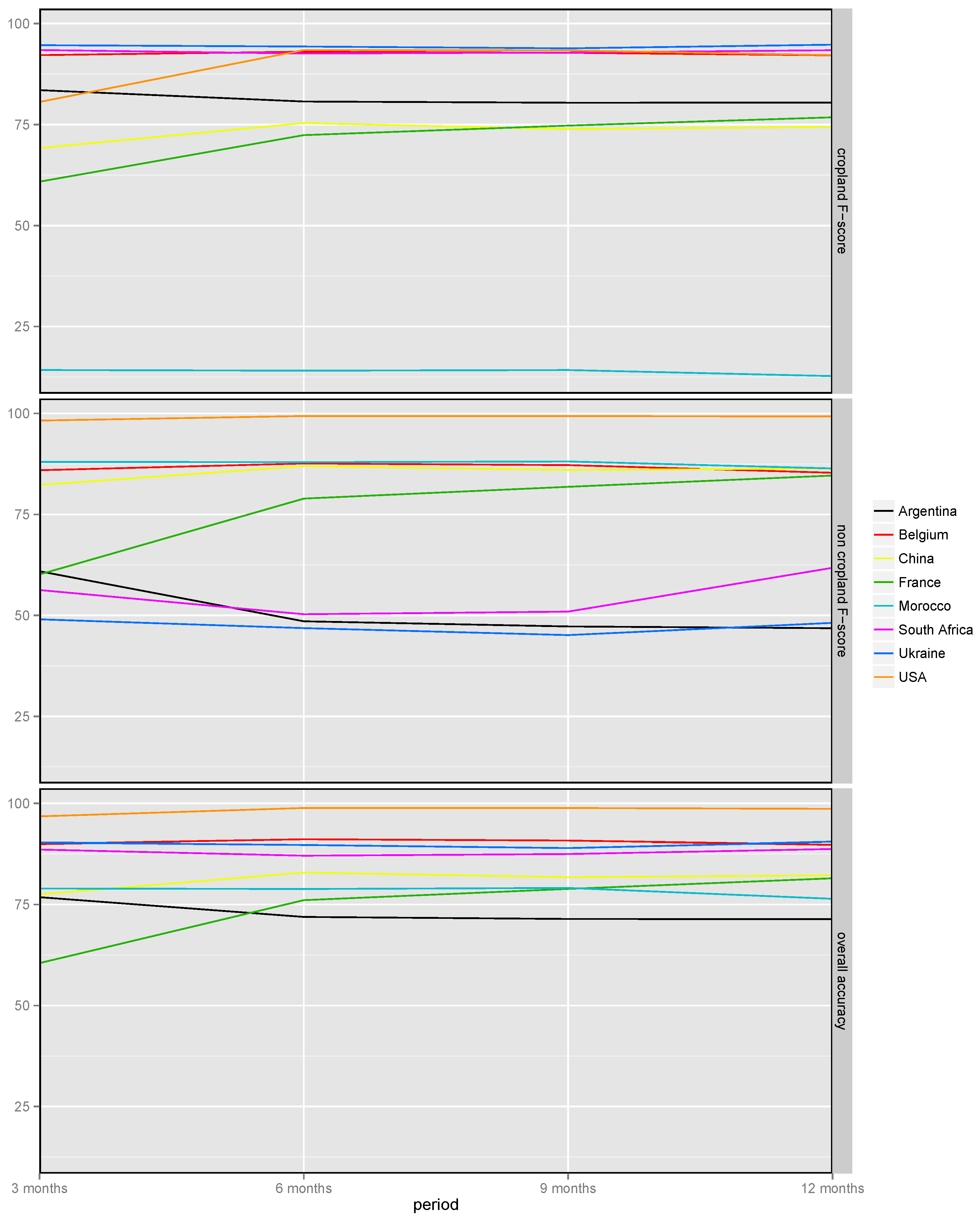
Figure 7 illustrates the saturation of the OAs six months after the start of the time series, when stable OA values were observed, and it was noted that additional EO data did not improve the results. This was quite meaningful for the Northern Hemisphere sites, as this period corresponded to August, when most of the crop cycles were being completed. This period also corresponded to the end of the Spot 4 Take 5 experiment, so only the Landsat-8 data were used for the rest of the season, providing less dense time series.
After the three-month period, the methodology produced cropland maps with accuracies that were higher than 75% for all sites, except France (OA of 65%). Such results are promising for analyzing shortened or fragmented time series, as is often the case in cloudy regions. The main proportion of the area detected as cropland by three out of the four cropland maps (blue areas in
Figure 6a,c,e) was linked to cropland not identified as such at the beginning of the time series (after three months). The sites located in the Southern Hemisphere provided the highest accuracies at the beginning of the time series and then tended to decrease slightly due to the mismatch between the growing season and the EO time series (
Figure 6a).
Figure 7.
Overall accuracy (OA), F-score for cropland and non-cropland classes as mapped by the maximum likelihood classifier, combined with trimming three, six, nine and twelve months after the beginning of the time series.
Figure 7.
Overall accuracy (OA), F-score for cropland and non-cropland classes as mapped by the maximum likelihood classifier, combined with trimming three, six, nine and twelve months after the beginning of the time series.
4.4. The Effect of Baseline Resolution
Previous results showed an impact on accuracy for sites for which a local high resolution baseline was available when using the K-means method (see
Section 4.1,
Table 5). With the exception of France, the test sites showed that OAs resulting from the use of a local high resolution baseline were very close to those obtained when using a global 300-m baseline (
Table 6), with a difference in accuracy of below 2%. The cropland and non-cropland precisions were both balanced. Nevertheless, the French site showed a loss of about 30% OA when using a global baseline, mainly because of a low precision for non-cropland. This discrepancy with the validation dataset was mainly present in the northeast of the site, where vineyards dominated the landscape.
Hence, using a global coarse baseline dataset does not significantly affect cropland mapping in comparison with the use of high resolution baseline datasets. Coarse resolution land cover maps are thus a viable source of prior land cover information available globally. This allows the methodology to be applied to any site and even over large areas that are not locally mapped.
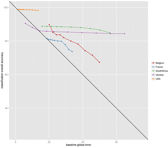
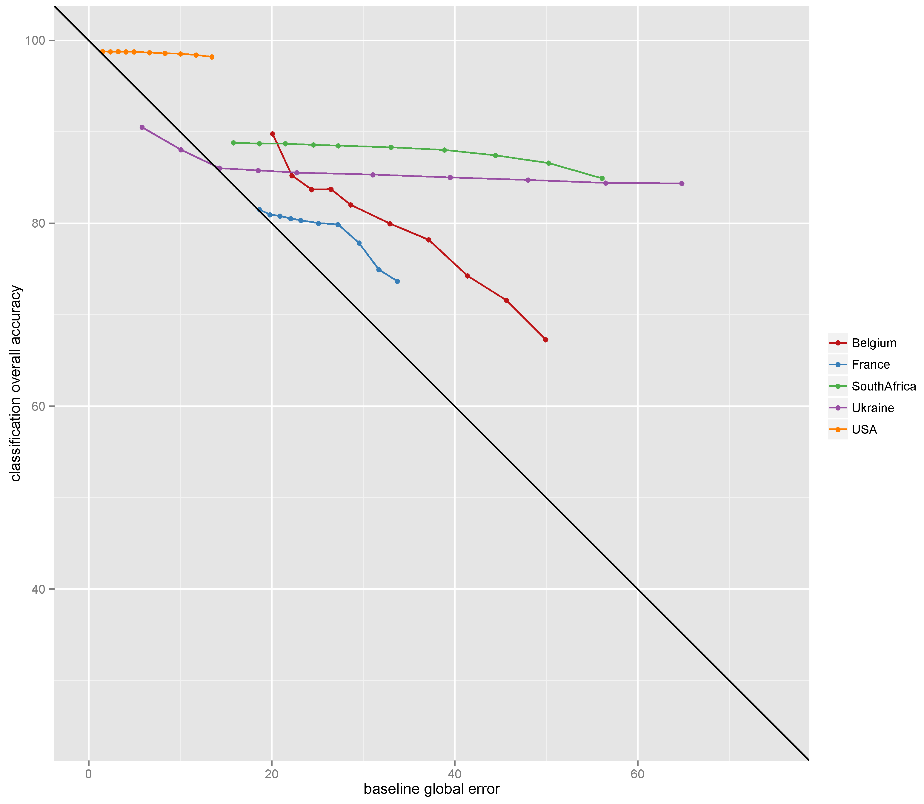
The noise added artificially to baselines affects the classification OA to a limited extent (
Figure 8). The noise is expressed in terms of global error (GE), defined as
. The lower impact is clearly visible in the USA, South Africa and Ukraine, where an increase of 60% of the baseline GE impacted the classification OA by only 5%. In Belgium and France, as the baseline GE increased, the classification OA decreased more than over the other sites. However, the classification OA reduction rate decreases as the baseline GE increases, demonstrating that the baseline GE’s impact progressively diminishes (
Figure 8). This shows some robustness of the method in terms of mislabeled pixels in the baseline. It is worth mentioning that two distinct classes of the baseline (
i.e., rainfed cropland and irrigated cropland) were used separately in Belgium and France to train the cropland classification output, thus making them more sensitive to noise because the initial number of pixels of the individual cropland class was heavily reduced.
Figure 8.
Effect of baseline global error (GE) () on classification overall accuracy (OA). Increasing baseline GE was linked to the artificially-added noise (the lower the noise, the lower the GE) and induced a classification OA decrease. The 1:1 line represents the same accuracy for both the baseline and the classification.
Table 6.
Impact of baseline resolution on accuracy. The“local” land cover information refers to locally available high resolution maps, while “global” refers to the 300-m CCI Land Cover dataset.
Table 6.
Impact of baseline resolution on accuracy. The“local” land cover information refers to locally available high resolution maps, while “global” refers to the 300-m CCI Land Cover dataset.
| Site | Overall Accuracy | Cropland Precision | Non-Cropland Precision |
|---|
| | Local | Global | Local | Global | Local | Global |
|---|
| Belgium | 89.8 | 90.9 | 90.1 | 93.2 | 98.2 | 87.1 |
| France | 81.5 | 56.2 | 92.7 | 90.6 | 92.3 | 44.4 |
| South Africa | 88.8 | 89.0 | 90.1 | 90.6 | 78.4 | 77.7 |
| Ukraine | 90.5 | 91.1 | 93.1 | 92.4 | 58.9 | 67.7 |
| USA | 98.6 | 98.2 | 91.3 | 86.0 | 99.3 | 99.5 |
5. Discussion
The automated methodology proposed for annual cropland mapping was independent of in situ data and proved to effectively differentiate the cropland (OA > 85%). The results showed that the most accurate approach included an iterative trimming of the baseline to extract training data, necessary for the calibration of a maximum likelihood classifier. The OA obtained for the eight sites distributed throughout the world ranged from 71%–99%, depending on the site, its agricultural landscape and the EO time series (six out of eight sites had an OA higher than 80%). These performances seem compatible with the expected use of a cropland mask in an operational agricultural monitoring system, i.e., masking out the non-cropland area to specifically monitor the crop growing condition along the season or to provide an early outlook on the cultivated area in a given region. For the latter application, an accuracy level of higher than 90% is most suitable and seems attainable for half of the sites.
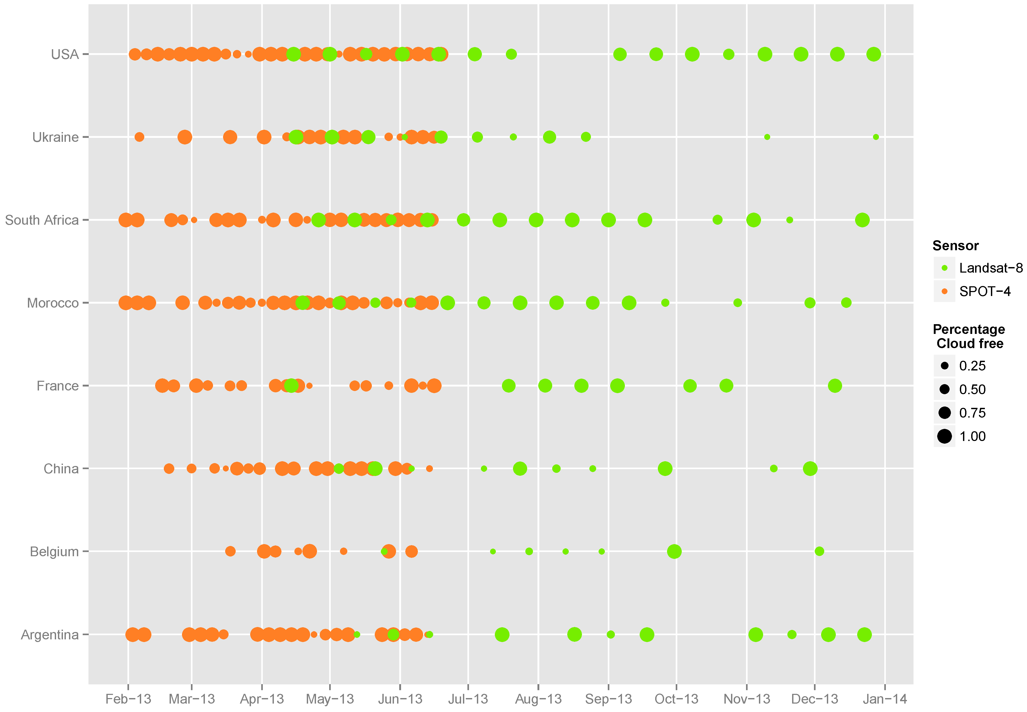
The large diversity of landscapes structures and the contrasted densities of EO time series (11 images in Belgium, 69 in the USA) did not prevent the methodology from delivering relevant results. Among the major agrosystems, rice was the only commodity not considered in this study. All major factors impacting cropland mapping were included in the dataset (i.e., cloudiness, unsynchronized crop cycles, crop diversity, parcel size, climate conditions and landscape homogeneity), making the demonstration of robustness quite convincing.
In most cases, the object-based versions of the methodology yielded similar or slightly better results than the pixel approach. As the segmentation is a computationally-intensive process, its added value ought to be balanced out carefully, and it represents a potential issue when considering large areas. Only two sites presented significant improvement when using objects instead of pixels as the spatial processing unit. The segmentation used was derived from the complete NDVI time series, which hampered information delivery along the season. An alternative would be to use objects from the previous year and to assume minor annual changes. Both the availability of an NDVI time series from the previous year and the limited cropland inter-annual variability constrained the extension of the methodology, especially in regions with high temporal variations in crop structures [
57].
The performance of the methodology and its independence from season field data collection and even from any
in situ data rely heavily on the trimming process. However, assumptions have to be met when using the trimming method for cleaning. First, the spectral reflectances corresponding to each class are assumed to fit a unimodal Gaussian distribution. This is not necessarily always the case, especially in regions with a large diversity of crop cycles, so spectrally-different pixels must be included in the same class, disabling the trimming outlier removal capabilities. However, this effect is limited by the use of the temporal features computed on each pixel reducing the spectral gap between crops. The second assumption concerns the quality of the existing land cover data, which should be valid for the majority of the pixels (
i.e., more than half of them). As the trimming is applied to each class separately, taking into account the information contained in the other classes could help in the case of a poor quality map [
58].
The automation and genericity of the methodology presented in this paper could be further improved by a local adjusted feature selection, taking into account the regional agricultural landscape characteristics. Indeed, the twenty possible features were reduced to five in order for the experiment to cope with Hughes’ phenomenon [
49]. The literature contains some clues, such as an adaptation of the maximum relevance minimum redundancy feature selection [
59,
60,
61], that would support a more specific feature selection. A so-called “optimum approach” might consist of an automated selection of features containing the most discriminating power between cropland and non-cropland pixels. This would enhance the methodology in terms of handling site specificity, making it more able to address global crop diversity.


 ,
, 


