1. Introduction
Soil moisture content and roughness play an important role in hydrology. These soil parameters could be estimated using Synthetic Aperture Radar (SAR) irrespective of the meteorological conditions. However, these estimations require the use of a radar backscattering model that is capable of correctly modeling the radar signal. The Integral Equation Model (IEM) [
1,
2] is widely used in inversion procedures of SAR images for retrieving soil moisture content and roughness (e.g., [
3,
4,
5,
6,
7,
8,
9]). Its validity domain covers the range of surface roughness values (root mean square height “
rms”) encountered on agricultural soils (
k.rms ≤ 3, where
k is the wave number = 0.24 cm
−1 for a frequency in L-band of 1.25 GHz).
The IEM simulates the radar backscattering coefficient (σ°) for bare soils given sensor parameters (radar wavelength, incidence angle, and polarization) and soil characteristics (dielectric constant, standard deviation of heights, correlation length, and autocorrelation function “ACF”). Most studies reported discrepancies between modeled backscatters by IEM and observed backscatters by SAR sensors at L-, C-, and X-bands [
10,
11,
12,
13,
14,
15,
16,
17,
18,
19,
20]. These discrepancies could be related to the inaccuracy of the roughness measurements, which introduces significant errors into the modeled radar signal [
21,
22], and to the model itself [
10,
11,
12,
13,
14,
15]. Indeed, according to Lievens
et al. [
21] and Oh and Kay [
22], correlation length measurements are unreliable when short roughness profiles are used or when the number of profiles is limited (error over 50%). Thus, the estimation of soil parameters (moisture content and roughness) from SAR images can be inaccurate using such a model.
Baghdadi
et al. [
10,
11,
12,
13,
14] proposed a semi-empirical calibration of the IEM at C- and X-bands, based on experimental data of SAR images and ground measurements (soil moisture content and roughness). The calibration consisted of finding a fitting parameter which replaces the correlation length measurement so that the IEM reproduces better the radar backscattering coefficient. Calibration results showed that the fitting parameter was found dependent on
rms surface height, radar wavelength, polarization, and incidence angle. Given the successful application at C- and X-bands, this paper aims at deriving similar equations for L-band.
The first objective of this study is to evaluate the IEM using dataset acquired over numerous study sites in Europe (France, Luxembourg, Belgium, Germany and Italy). Simulated backscattering coefficients from the IEM will be compared to the backscattered signal registered by several SAR systems at L-band and HH and VV polarizations (AIRSAR, SIR-C, JERS-1, PALSAR-1, ESAR). Next, a semi-empirical calibration of the IEM is proposed as was already derived by previous studies for C- and X-bands SAR data in order to improve the modeling of the radar signal by the IEM.
Section 2 describes the dataset. In
Section 3, a comparison between modeled and observed backscatters is presented. The semi-empirical calibration methodology of the IEM is proposed in
Section 4 and its performance evaluated in
Section 5. A summary of the results is provided in the last
Section 6.
2. Dataset Description
Experimental dataset of SAR images and measurements of soil moisture content and roughness acquired over bare soils were used. This dataset was collected over numerous agricultural study sites in France (2 sites), Luxembourg (1 site), Belgium (2 sites), Germany (1 site), and Italy (2 sites) (
Figure 1,
Table 1).
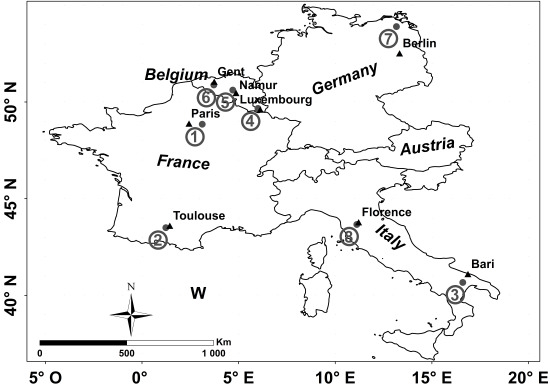
Figure 1.
Location of various study sites. “1”: Orgeval; “2”: Saint Lys; “3”: Matera; “4”: Alzette; “5”: Dijle; “6”: Zwalm; “7”: Demmin; “8”: Montespertoli.
Figure 1.
Location of various study sites. “1”: Orgeval; “2”: Saint Lys; “3”: Matera; “4”: Alzette; “5”: Dijle; “6”: Zwalm; “7”: Demmin; “8”: Montespertoli.
SAR images were acquired by various airborne and spaceborne sensors (AIRSAR, SIR-C, JERS-1, PALSAR-1, ESAR) operating at L-band (~1.25 to 1.30 GHz), with incidence angles between 21.5° and 57°, and in HH and VV polarizations. For experimental bare soil plots, the mean backscattering coefficients are calculated from calibrated SAR images by linearly averaging the σ° values of all pixels within the plot. Only plots with a homogeneous surface (similar soil type, moisture content and surface roughness) of around one hectare or more (about 100 pixels for SAR images with a spatial resolution of 10 m × 10 m) were used (which helps reducing speckle). In addition,
in situ ground measurements of soil moisture content (
mv) and roughness were carried out for each experimental plot. The soil moisture measurements were collected from the top 5 or 10 cm of each experimental plot using the gravimetric method or/and a calibrated TDR (Time Domain Reflectometry) probe. For wet soil conditions, the soil moisture measurements were collected from the top 5 cm and from the top 10 cm for dry soil conditions. Nolan and Fatland [
23] found that in a clay loam soil, the penetration depth of L-band radar signals decreased from approximately 10 cm in the case of 5 vol % soil moisture content, to 5 cm when the soil moisture content increased to 15 vol %. In practice, the soil moisture for each experimental plot is assumed to be equal to the mean value measured from several samples (the number of soil moisture samples depends on the size of experimental plots). The single-field standard deviation of soil moisture is lower than 2 vol % for 95% of the measurements.
Table 1.
Main characteristics of the dataset used in this study.
Table 1.
Main characteristics of the dataset used in this study.
| Site | Lat/Long | Texture Composition (Silt; Clay; Sand) | SAR Sensor | Pixel Spacing (m × m) | Freq (GHz) | Year | Number of Data for Each SAR Configuration |
|---|
| Orgeval (Fr) [24] | 48°51′ N 3°07′ E | (78%; 17%; 5%) | SIR-C | 12.5 × 12.5 | 1.25 | 1994 | HH: 52° (5), 55° (5), 57° (5)
VV: 52° (5), 55° (5), 57° (5) |
| Orgeval (Fr) | 48°51′ N 3°07′ E | (78%; 17%; 5%) | PALSAR-1 | 12.5 × 12.5 | 1.27 | 2009 | HH: 21.5° (7)
VV: 21.5° (7) |
| Saint Lys (Fr) [25] | 43°30′ N 01°14′ E | (50%; 16%; 34%) | PALSAR-1 | 6.25 × 6.25
12.5 × 12.5 | 1.27 | 2010 | HH: 38.7° (15) |
| Matera (It) [17] | 40°40′ N 16°36′ E | (59%; 14%; 27%) | SIR-C | 12.5 × 12.5 | 1.25 | 1994 | HH: 45.8° (6)
VV: 45.8° (6) |
| Alzette (Lu) [26] | 49°40′ N 06°00′ E | (50%; 30%; 20%) | PALSAR-1 | 12.5 × 12.5 | 1.27 | 2008 | HH: 36.5°–41.1° (4) |
| Dijle (Be) [26] | 50°37′ N 04°42′ E | (84%; 12%; 4%) | PALSAR-1 | 12.5 × 12.5 | 1.27 | 2008; 2009 | HH: 36.2°–39.4° (12) |
| Zwalm (Be) [26] | 50°53′ N 03°43′ E | (72%; 13%; 15%) | PALSAR-1 | 12.5 × 12.5 | 1.27 | 2007 | HH: 38.7° (2) |
| Demmin (Ge) [26] | 53°54′ N 13°10′ E | (25%; 7%; 68%) | ESAR | 2 × 2 | 1.30 | 2006 | HH: 40°–48.4° (9) |
| Montespertoli (It) [27] | 43°40′ N 11°7′ E | (40%; 20%; 40%) | AIRSAR | 12.5 × 12.5 | 1.26 | 1991 | HH: 25° (7), 35° (7), 50° (7)
VV: 25° (7), 35° (7), 50° (7) |
| Montespertoli (It) [28] | 43°40′ N 11°7′ E | (40%; 20%; 40%) | SIR-C | 12.5 × 12.5 | 1.25 | 1994 | HH: 25° (25), 35° (8), 45° (22)
VV: 25° (25), 35° (8), 45° (8) |
| Montespertoli (It) [29] | 43°40′ N 11°7′ E | (40%; 20%; 40%) | JERS-1 | 12.5 × 12.5 | 1.27 | 1994 | HH: 35° (8) |
Roughness measurements are made using laser or needle profilometers (1, 2 and 3 m long and with 0.5, 1, 1.5, and 2 cm sampling intervals) and meshboard (4 m long) with several roughness profiles for each experimental plot, parallel and perpendicular to tillage direction. From these roughness measurements, the root mean square (rms) surface height and the correlation length (L) are calculated using the mean of all ACFs.
The
in situ measurements accuracy of
rms and
L depends on the roughness profile length and sampling interval (e.g., [
21,
22,
30]). In our database, the roughness parameter
rms has been estimated with an accuracy ranging between 5% and 10%, and the
L-values with an accuracy ranging between 10% and 20% [
20,
21]. Low uncertainties on the roughness parameters measurements are obtained for high length and low sampling interval of the roughness profiles.
Soil moisture, rms surface height, and correlation length range respectively from 3.5 to 40.9 vol %, 0.65 to 9.55 cm, and from 2.37 to 38.50 cm. A total of 154 experimental data points is available in HH and 90 in VV.
3. Evaluation of the IEM
The Integral Equation Model (IEM) developed by Fung
et al. [
1] is a theoretical radar backscattering model that is widely used for soil moisture content and roughness estimation. At L-band, the IEM has a validity domain that covers the range of roughness values that are commonly encountered for agricultural surfaces. The IEM simulates the radar backscattering coefficient from the radar wavelength, the incidence angle, the polarization, the soil
rms surface height, the soil correlation length, the ACF, and the soil dielectric constant derived from the moisture content and the soil texture [
31]. Over bare soils in agricultural areas, the ACF is exponential for low soil roughness values and Gaussian for high soil roughness values [
2].
Table 2.
Statistics for the evaluation of Integral Equation Model (IEM). Bias = SAR–IEM; MAE = Mean Absolute Error; RMSE = Root Mean Square Error.
Table 2.
Statistics for the evaluation of Integral Equation Model (IEM). Bias = SAR–IEM; MAE = Mean Absolute Error; RMSE = Root Mean Square Error.
| Polarization | Autocorrelation Function | Bias (dB) | MAE (dB) | RMSE (dB) |
|---|
| HH | Exponential; all rms values | +0.4 | 2.5 | 3.2 |
| Exponential; rms < 3 cm | +0.6 | 2.2 | 2.9 |
| Exponential; rms > 3 cm | −0.3 | 3.2 | 3.9 |
| HH | Gaussian; all rms values | −1.2 | 2.9 | 3.8 |
| Gaussian; rms < 3 cm | −0.5 | 2.7 | 3.9 |
| Gaussian; rms > 3 cm | −2.7 | 3.1 | 3.7 |
| VV | Exponential; all rms values | −1.2 | 3.0 | 3.7 |
| Exponential; rms < 3 cm | −2.2 | 2.9 | 3.5 |
| Exponential; rms > 3 cm | +1.6 | 3.5 | 4.1 |
| VV | Gaussian; all rms values | −2.5 | 3.9 | 5.0 |
| Gaussian; rms < 3 cm | −2.8 | 4.4 | 5.6 |
| Gaussian; rms > 3 cm | −1.8 | 2.5 | 3.2 |
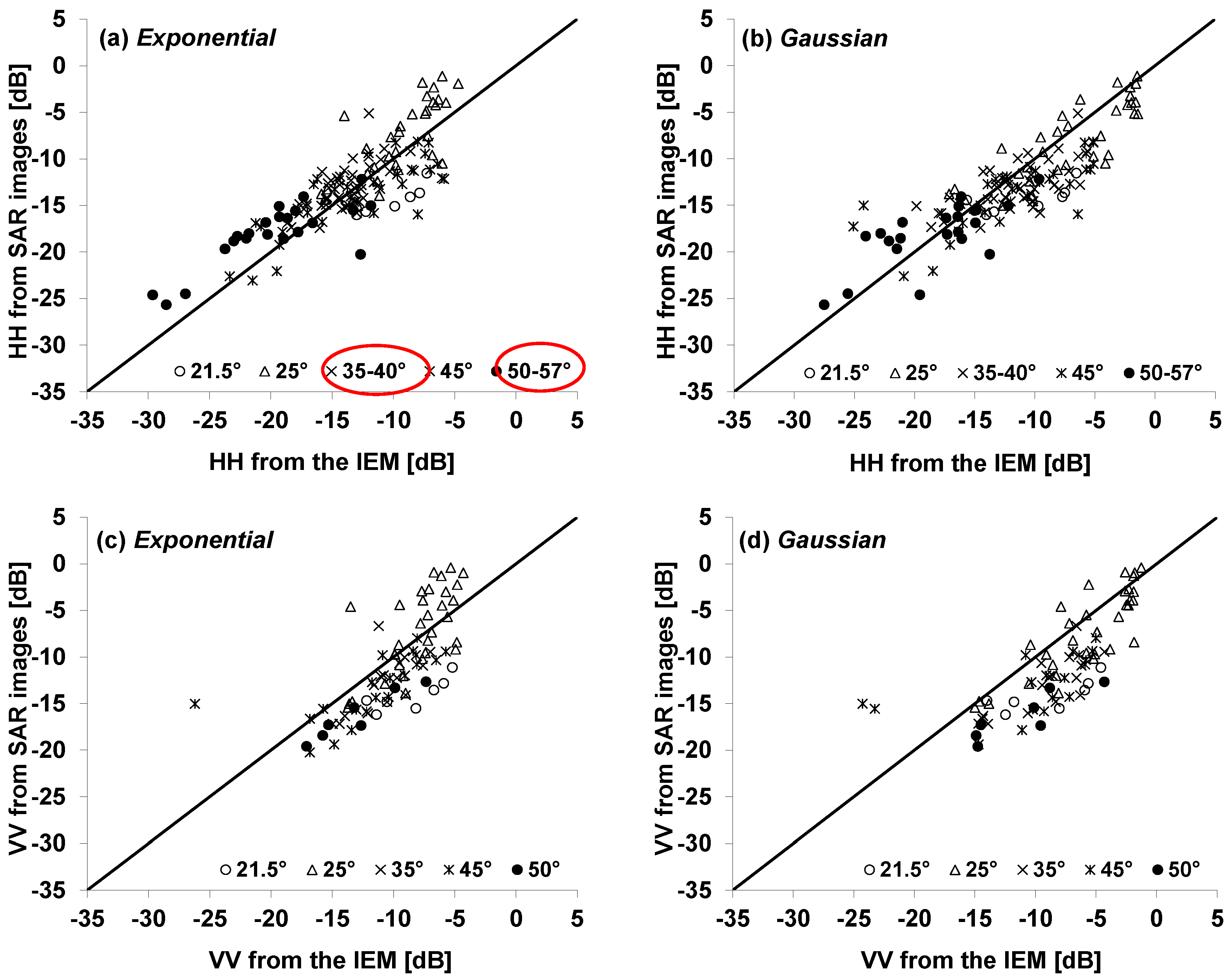
Comparison between the IEM simulations and the experimental dataset was done for both exponential and Gaussian ACFs (
Table 2,
Figure 2). Simulation results were slightly better with the exponential ACF than with the Gaussian ACF. Similarly, HH provides slightly better results than VV. With the exponential ACF, the mean difference between experimental data and IEM simulations is +0.4 dB in HH and −1.2 dB in VV with an RMSE about 3.5 dB (3.2 in HH and 3.7 dB in VV). The use of Gaussian ACF causes higher biases in comparison to the exponential ACF (−1.2 dB in HH and −2.5 dB in VV), and RMSE of the same order of magnitude in HH (3.8 dB) but higher in VV (5.0 dB). Other studies have reported a tendency of the IEM to overestimate observed L-band backscatter values [
16,
17].
Figure 2.
Observed backscatter coefficients from Synthetic Aperture Radar (SAR) images (L-band) vs. modeled backscatter values from IEM (at different incidence angles) using correlation length measurements, for exponential and Gaussian autocorrelation function (ACFs). Mean of the difference between SAR and IEM and root mean square error were calculated for all rms values. (a): HH polarization and exponential ACF, (b): HH polarization and Gaussian ACF, (c): VV polarization and exponential ACF, (d): VV polarization and Gaussian ACF.
Many studies used for validation the IEM show an even more limited validity domain
k.rms < 1 [
24,
32] than the one defined initially by Fung
et al. [
1,
2]
k.rms < 3. Consequently, the error in the modeling of radar backscattering coefficients was also analyzed as a function of
rms surface height classes (
rms < 3 cm and
rms > 3 cm, corresponding to
k.rms < 1). Results showed that the exponential ACF provides better IEM simulations for values of
rms lower than 3 cm (RMSE = 2.9 dB for HH and 3.5 dB for VV with the exponential ACF, and RMSE = 3.9 dB for HH and 5.6 dB for VV with the Gaussian ACF) (
Table 2). For values of
rms greater than 3 cm, the use of Gaussian ACF is more relevant (RMSE = 3.7 dB for HH and 3.2 dB for VV with the Gaussian ACF, and RMSE = 3.9 dB for HH and 4.1 dB for VV with the exponential ACF) (
Table 2).
4. IEM Semi Empirical Calibration Methodology
The description of surface roughness in the IEM is based on three parameters: the
rms surface height, the correlation length, and the ACF. As the modeled backscattering coefficient depends on the shape of the ACF chosen, the use of the IEM in operational mode for estimating the soil moisture content from SAR images, at a given spatial scale (sub-plot, plot,
etc.), requires knowledge on the ACF shape which depends on the
rms surface height value (generally exponential for smooth surfaces and Gaussian for rough surfaces). As the
rms values are also unknown during model inversion, it is therefore difficult to choose the required ACF, which therefore would lead to an inaccurate retrieval of the soil moisture. In fact, the use of the unsuitable autocorrelation function leads to important errors on the backscattering coefficients estimation. For
rms lower than 3 cm, the use of Gaussian ACF instead of an exponential ACF leads to an error increase up to 2.1 dB on the retrieval of backscattering coefficients (
Table 2).
For
rms greater than 3 cm, the use of exponential ACF instead of Gaussian ACF leads to an error increase up to 0.9 dB (
Table 2). Consequently, an additional uncertainty on the retrieval of backscattering coefficients of only 1 dB may lead to additional uncertainty on the soil moisture estimates by about 5 vol % for sensitivity of radar signal in L-band of 0.2 dB for 1 vol % [
33].
Moreover, the measurements of correlation length are often the less accurate in comparison to other measured soil parameters [
21,
22], and the discrepancies noted between IEM simulations and SAR data could be attributed to the uncertainty of the correlation length measurements and to the model itself [
10,
13,
14,
15]. Thus, the semi empirical calibration of the IEM consisted in the replacement of the experimental correlation length by a fitting parameter in order to ensure better matching between simulations and SAR data [
10,
13,
14]. In Baghdadi
et al. [
10,
13,
14], the calibration parameter was found to be dependent on surface roughness, incidence angle, polarization, and radar wavelength. In addition, with this Baghdadi calibration method, bare soils will be characterized by two surface parameters (
rms surface height and moisture content) instead of three (
rms surface height, correlation length and moisture content), in case the ACF is predefined for the entire range of
rms surface heights.
Given the robustness of the IEM semi-empirical calibration proposed in Baghdadi
et al. [
10,
14] for C- and X-bands SAR data as demonstrated in (e.g., [
16,
18,
20]), the objective is to extend the same approach to L-band in order to improve the SAR backscatter prediction. The prediction error on the radar backscattering coefficients based on a 10-fold cross-validation was estimated for each polarization in order to validate the predictive performance of the calibrated version of the IEM (dataset was randomly divided into 90% training and 10% validation data elements and this procedure was repeated 10 times).
The method consists of replacing for each training data element the experimental correlation length by a fitting parameter (Lopt) which ensures a good fit between the backscattering coefficient provided by the SAR sensor and that simulated by the IEM. This approach considers the same correlation function irrespective to the range of rms surface height.
5. Results and Discussion
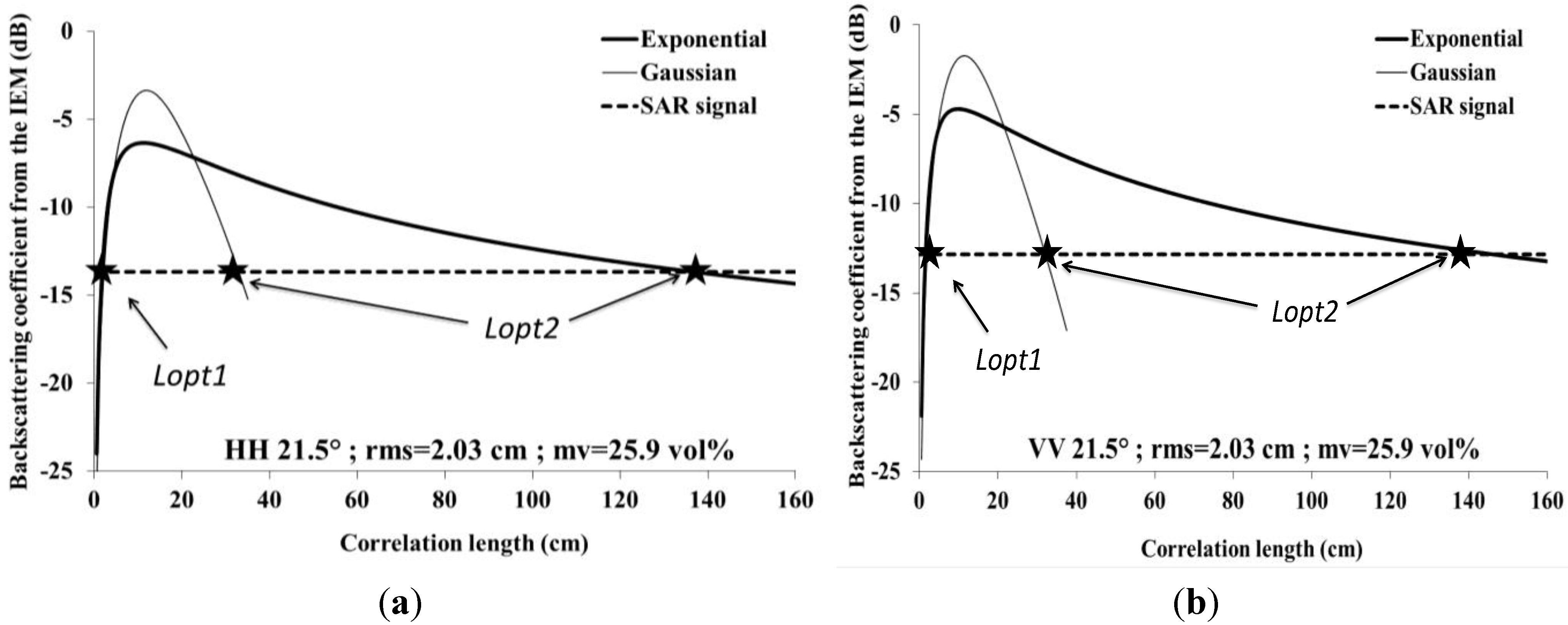
Figure 3 shows the behavior of the IEM as a function of the correlation length, for the exponential and Gaussian ACFs. As illustrated,
Lopt has two possible solutions,
Lopt1 (the lowest value) and
Lopt2 (the highest value). Results showed that
Lopt1 values in HH were higher than those in VV for both exponential and Gaussian ACFs, whereas
Lopt2 values were similar in HH and VV for both ACFs. Increasing of IEM in the first part of simulations corresponds to very short correlation lengths. For these short
Lopt-values, the IEM is out of its validity domain [
1] (
Figure 4). Only the second part, with a decrease of the radar signal when the correlation length increases, corresponds to IEM validity domain (
Figure 4). Thus, only
Lopt2 can be retained. In addition, when we consider realistic correlation lengths for agricultural soils (approximately higher than 3 cm), we observe a decreasing of radar signal in L, C and X bands as the correlation length increases. However, for lower frequencies, like P band, we observe clearly an increasing of radar signal function of correlation length.
Figure 3.
Behaviour of the IEM as a function of correlation length for a given plot, with Gaussian and exponential ACFs. (a): HH polarization, (b): VV polarization.
Figure 3.
Behaviour of the IEM as a function of correlation length for a given plot, with Gaussian and exponential ACFs. (a): HH polarization, (b): VV polarization.
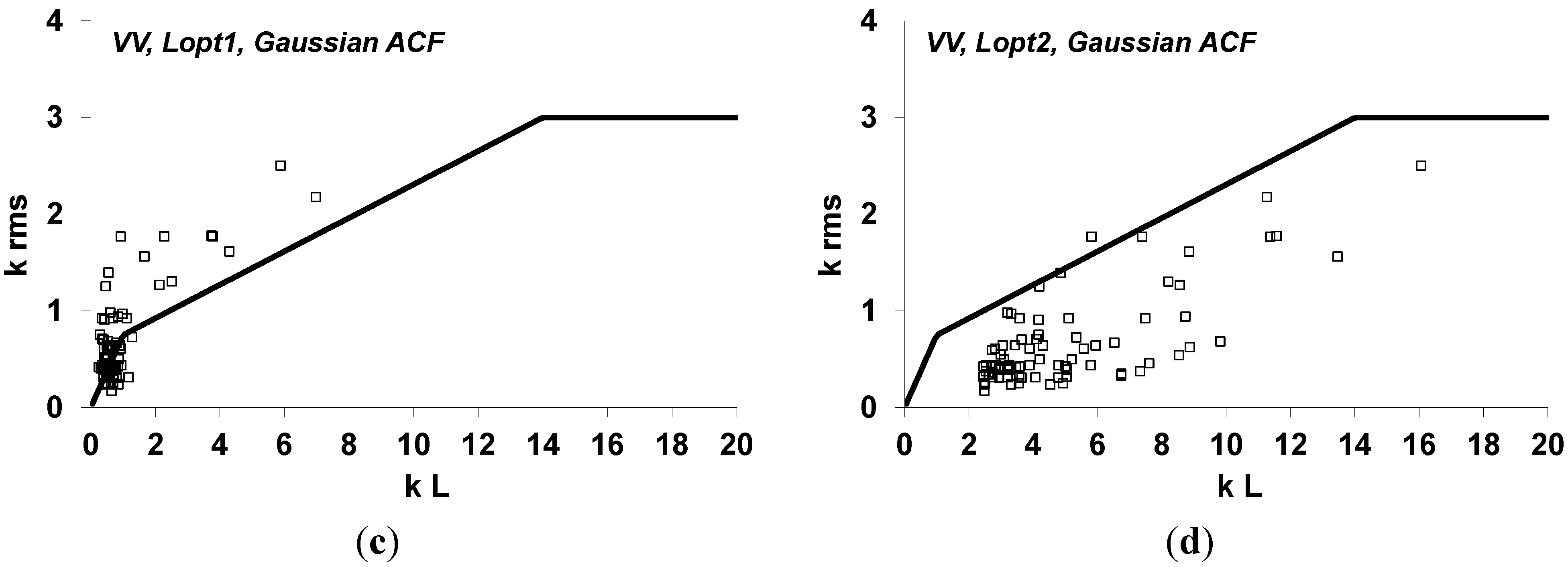
Figure 4.
Validity regions of the IEM model in
k.rms -
L space (where
k is the wave number) for Gaussian ACF, and the location of experimental data points [
1]. All experimental data points are within the IEM limits with
Lopt2. (
a): HH polarization and
L=
Lopt1, (
b): HH polarization and
L=
Lopt2, (
c): VV polarization and
L=
Lopt1, (
d): VV polarization and
L=
Lopt2.
For each dataset element, the fitting procedure has a higher probability to find an estimation of
Lopt2 for the Gaussian ACF than for the exponential ACF since the σ° simulated from the IEM has a higher amplitude for the Gaussian ACF (
Figure 3). Therefore, the probability of intersecting the SAR signal with the IEM response is higher for the Gaussian ACF. Thus, our set of
Lopt2 data, calculated for each polarization, is consequently larger with the Gaussian ACF which justifies its use to fit the best regressions between
Lopt2 and
rms height as a function of incidence angle and polarization. A linear relationship between
Lopt2 with the Gaussian ACF and
rms (α + β
rms; α and β are dependent on polarization and incidence angle “θ”) ensures a correct modeling of the physical behavior of the IEM (σ° increases with
rms surface height for the whole range of
rms-values):
θ is in radian, Lopt2 and rms are in cm. The coefficients given in Equations (1) and (2) were derived using the entire dataset. However, during the cross-validation, coefficients were calculated using the associated training dataset.
For subsequent applications, Lopt2 obtained with the Gaussian ACF (Equations (1) and (2)) replaces the experimental correlation length in the IEM.
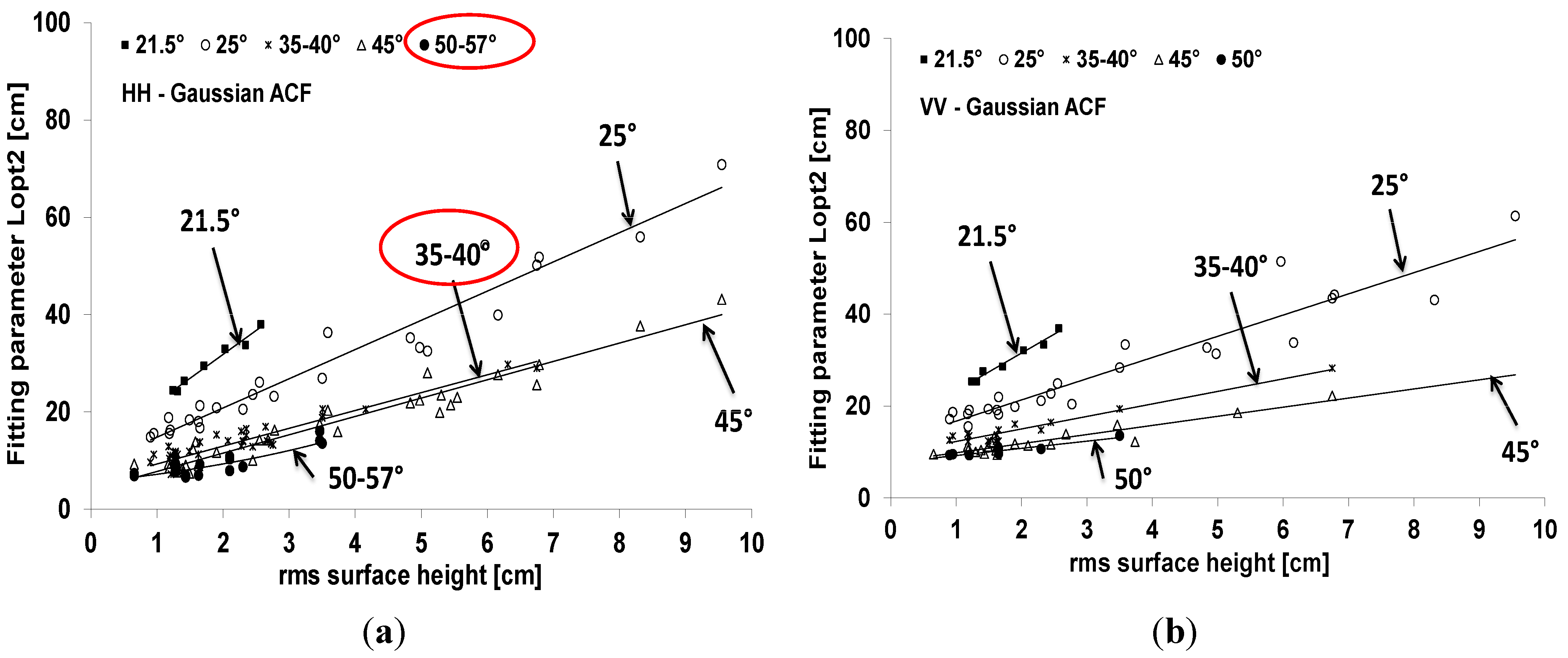
Figure 5 shows the fitting parameter
Lopt2 obtained with the Gaussian ACF. Results showed that the fitting parameter
Lopt2 is strongly dependent on
rms surface height and the incidence angle. It increases as the
rms increases and decreases with the incidence angle (
Figure 5). The dependence between
Lopt2 and the incidence angle becomes weak for θ > 35°. In addition,
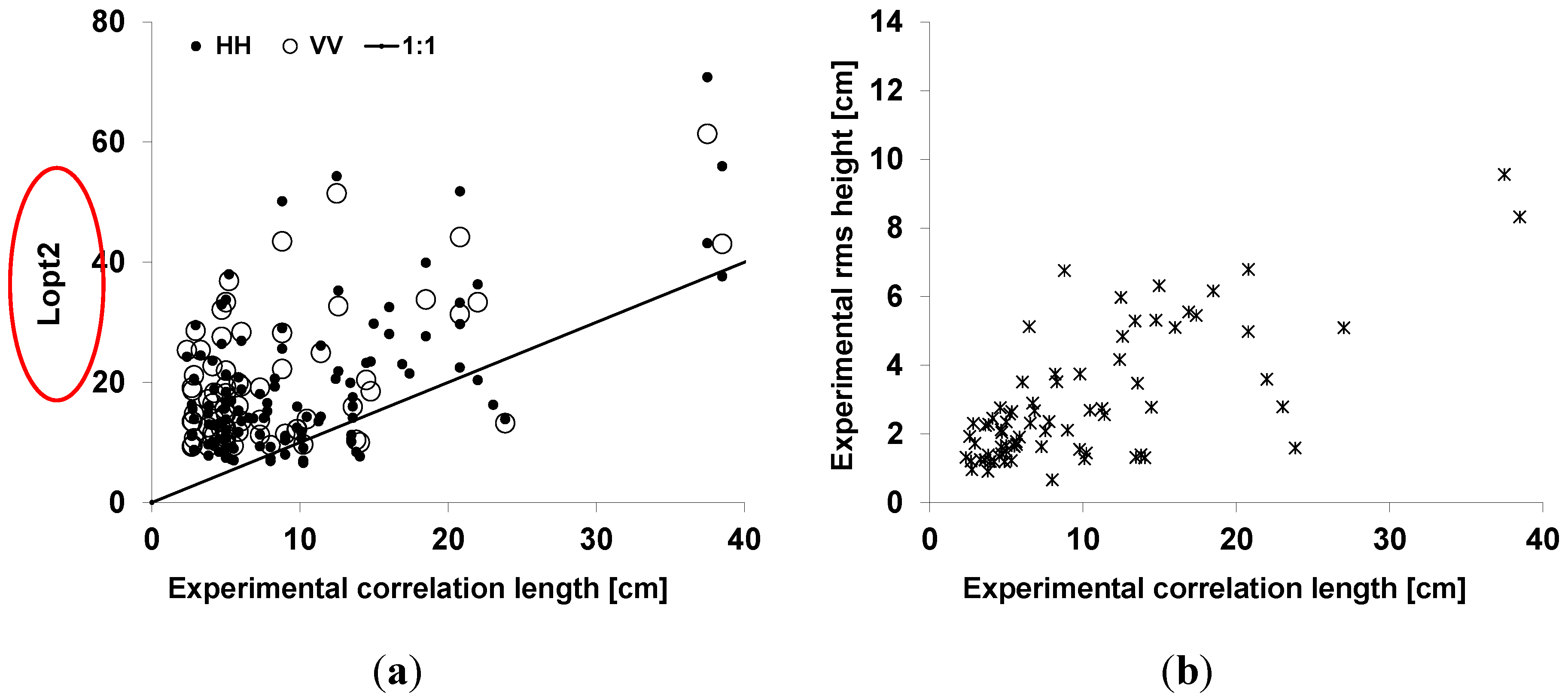
Figure 6a shows that the fitting parameter
Lopt2 is higher than the experimental correlation length and that
Lopt2 is similar for HH and VV polarizations. The experimental correlation length also showed an increase with the
rms surface height (
Figure 6b).
Figure 5.
Fitting parameter Lopt2 as a function rms surface height with the Gaussian ACF. (a): HH polarization, (b) VV polarization.
Figure 5.
Fitting parameter Lopt2 as a function rms surface height with the Gaussian ACF. (a): HH polarization, (b) VV polarization.
Figure 6.
Relationship between (a) Lopt2 with Gaussian ACF and the experimental correlation length; (b) the root mean square surface height and the experimental correlation length obtained from in situ measurements.
Figure 6.
Relationship between (a) Lopt2 with Gaussian ACF and the experimental correlation length; (b) the root mean square surface height and the experimental correlation length obtained from in situ measurements.
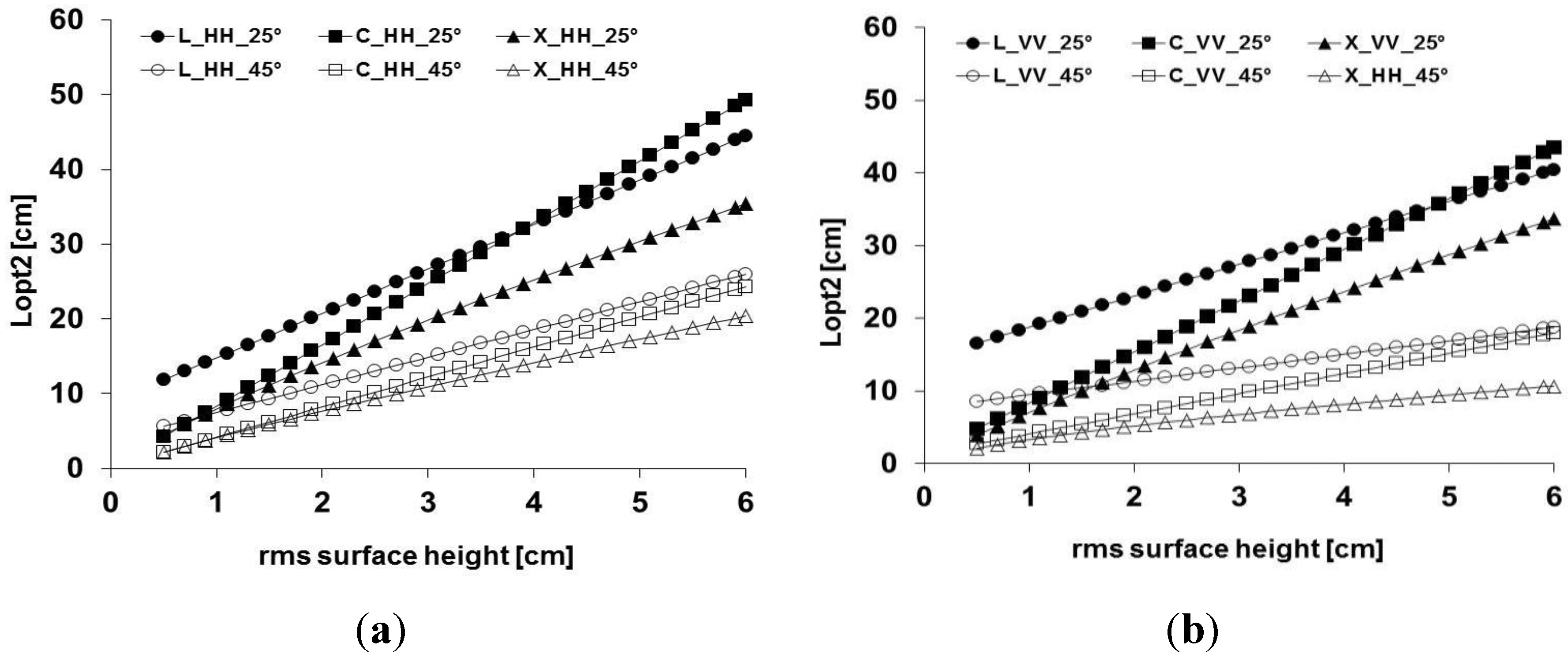
The effect of the radar frequency on the IEM calibration was done by comparing the expressions of
Lopt2 obtained by Baghdadi
et al. [
12,
14] and Zribi and Baghdadi [
34] at C- and X-bands to those obtained in this study for L-band (
Figure 7). Results showed that
Lopt2 increases as the radar wavelength increases.
Figure 7.
Comparison between
Lopt2 obtained in this study for L-band and those obtained in previous studies for C- and X-bands [
12,
14,
34]. Gaussian ACF was used. (
a) HH; (
b) VV.
Figure 7.
Comparison between
Lopt2 obtained in this study for L-band and those obtained in previous studies for C- and X-bands [
12,
14,
34]. Gaussian ACF was used. (
a) HH; (
b) VV.
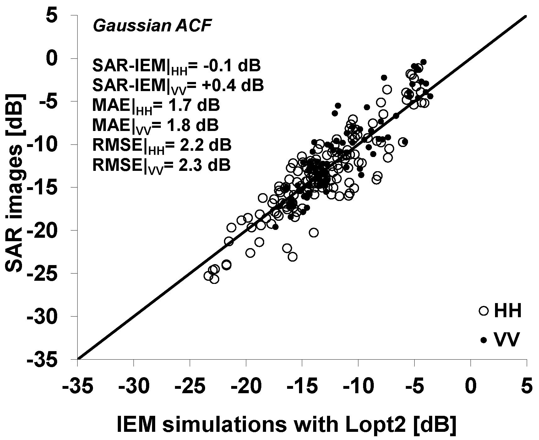
Finally, to validate the generalization performance of
Lopt2 (Equations (1) and (2)), a 10-fold cross validation was used. The error in the modeling of radar backscattering coefficients by the calibrated version of the IEM was assessed. Results showed that the proposed semi-empirical calibration of the IEM provides improved results (
Figure 8 in comparison to
Figure 2 and
Table 2). The biases and the RMSE have decreased for both HH and VV polarizations. The RMSE decreased from 3.2 dB with the exponential ACF and 3.8 dB with the Gaussian ACF to 2.2 dB for HH, and from 3.7 dB with the exponential ACF and 5.0 dB with the Gaussian ACF to 2.3 dB for VV (
Table 2,
Figure 8). We observe a small mean difference between SAR data and calibrated IEM simulations for both polarizations (less than 0.5 dB). In addition, the mean absolute error (MAE) was significantly reduced in using the fitting parameter
Lopt2 (
Table 2;
Figure 8). The cross-validation was also considered by changing the percentages of training and validation datasets: 90% for training and 10% for validation, 80% for training and 20% for validation, and finally 50% for training and 50% for validation). The results obtained on the prediction error of the radar backscattering were similar (difference lower than 0.2 dB).
Figure 8.
Validation of the semi-empirical calibration approach in using the fitting parameter Lopt2. Mean of the difference between SAR and IEM and root mean square error were calculated.
Figure 8.
Validation of the semi-empirical calibration approach in using the fitting parameter Lopt2. Mean of the difference between SAR and IEM and root mean square error were calculated.
In order to demonstrate the calibration method relevance on study sites that were not used in the calibration dataset, we then made a k-fold cross validation where k is the number of study sites (k = 11 for HH polarization and k = 5 for VV polarization). For each of k study sites, (k - 1) folds were used for training and the remaining one for testing. The advantage of this k-fold cross validation is that all the study sites in the dataset are used for both training and testing. Results showed similar results with an RMSE on the backscattering coefficient estimates of 2.2 dB for HH and 2.4 for VV.
6. Conclusions
The Integral Equation Model (IEM) was evaluated using L-band SAR data (HH and VV polarizations, incidence angles between 21.5° and 57°) together with in situ measurements (soil moisture and surface roughness) on bare soils in agricultural environments. A large dataset collected over numerous agricultural study sites in France, Luxembourg, Belgium, Germany and Italy using various SAR sensors (AIRSAR, SIR-C, JERS-1, PALSAR-1, ESAR) were used.
Simulation results were slightly better with exponential autocorrelation function than with Gaussian function. Similarly, HH provides slightly better results than VV. With the exponential function, the mean difference between SAR data and IEM simulations reaches −1.2 dB in VV with an RMSE of 3.7 dB. Simulations performed with the Gaussian function show biases of −1.2 dB in HH and −2.5 dB in VV, and RMSE of 3.8 dB in HH and 5.0 dB in VV.
A semi-empirical calibration of the IEM was proposed in order to improve the fitting of the IEM simulations to SAR response in HH and VV polarizations. Similar to approaches for C- and X-bands, the dependence of the fitting parameter on
rms surface height, incidence angle, polarization, and radar wavelength is found for L-band. With this calibration, agricultural bare soils can be characterized by only two surface parameters (
rms height and soil moisture) instead of four (
rms height, correlation length, autocorrelation function, and soil moisture) since the soil correlation length is replaced by a fitting parameter for a Gaussian ACF. Results showed that this calibration ensures better agreement between IEM and the SAR data and increases the model’s applicability (an improvement which can reach 3 dB for RMSE and 2 dB for MAE). Indeed, the decrease in error on the modeling of the SAR signal of about 1 dB will allow for improving the soil moisture estimates at least 3 vol % if we consider the sensitivity of the radar signal to soil moisture of about 0.3 dB/vol % [
35].


 ,
, 


