
The Use of Stereoscopic Satellite Images to Map Rills and Ephemeral Gullies


Abstract
:
1. Introduction
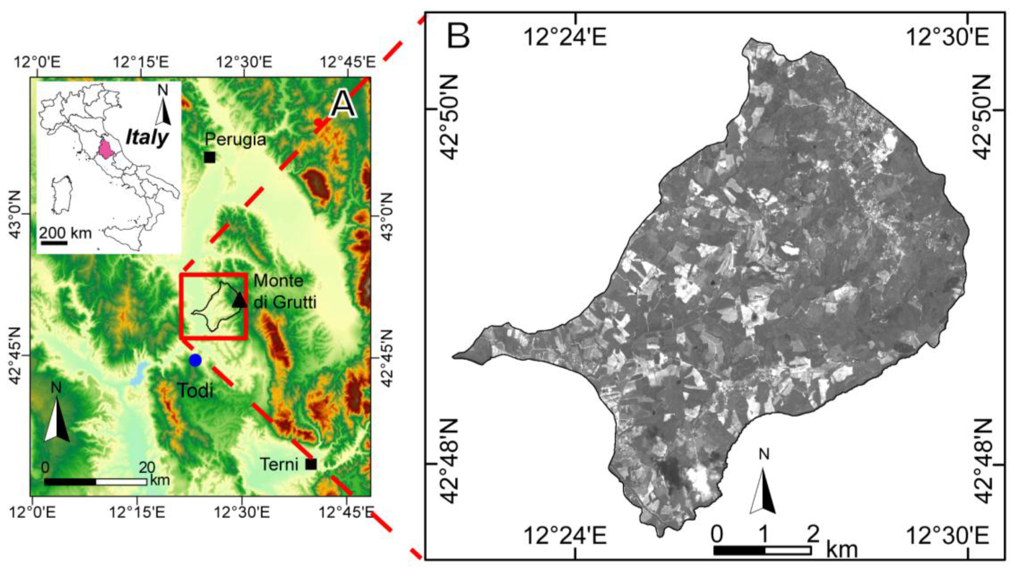
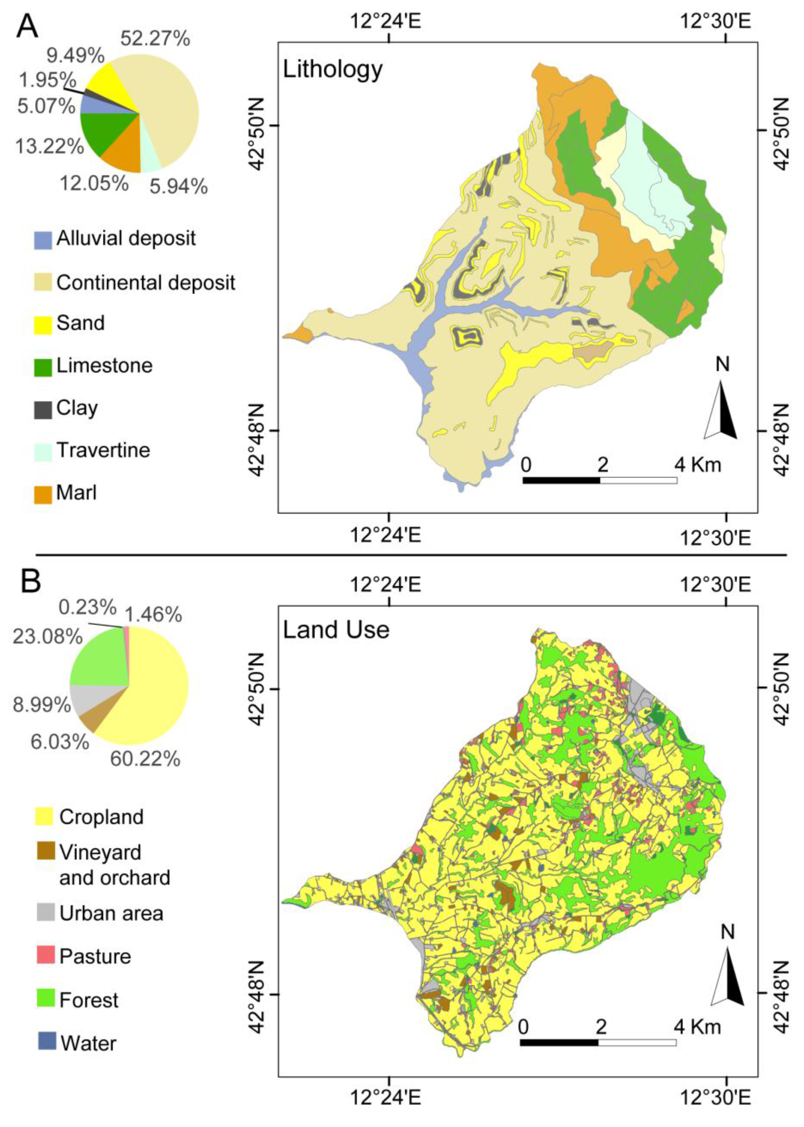
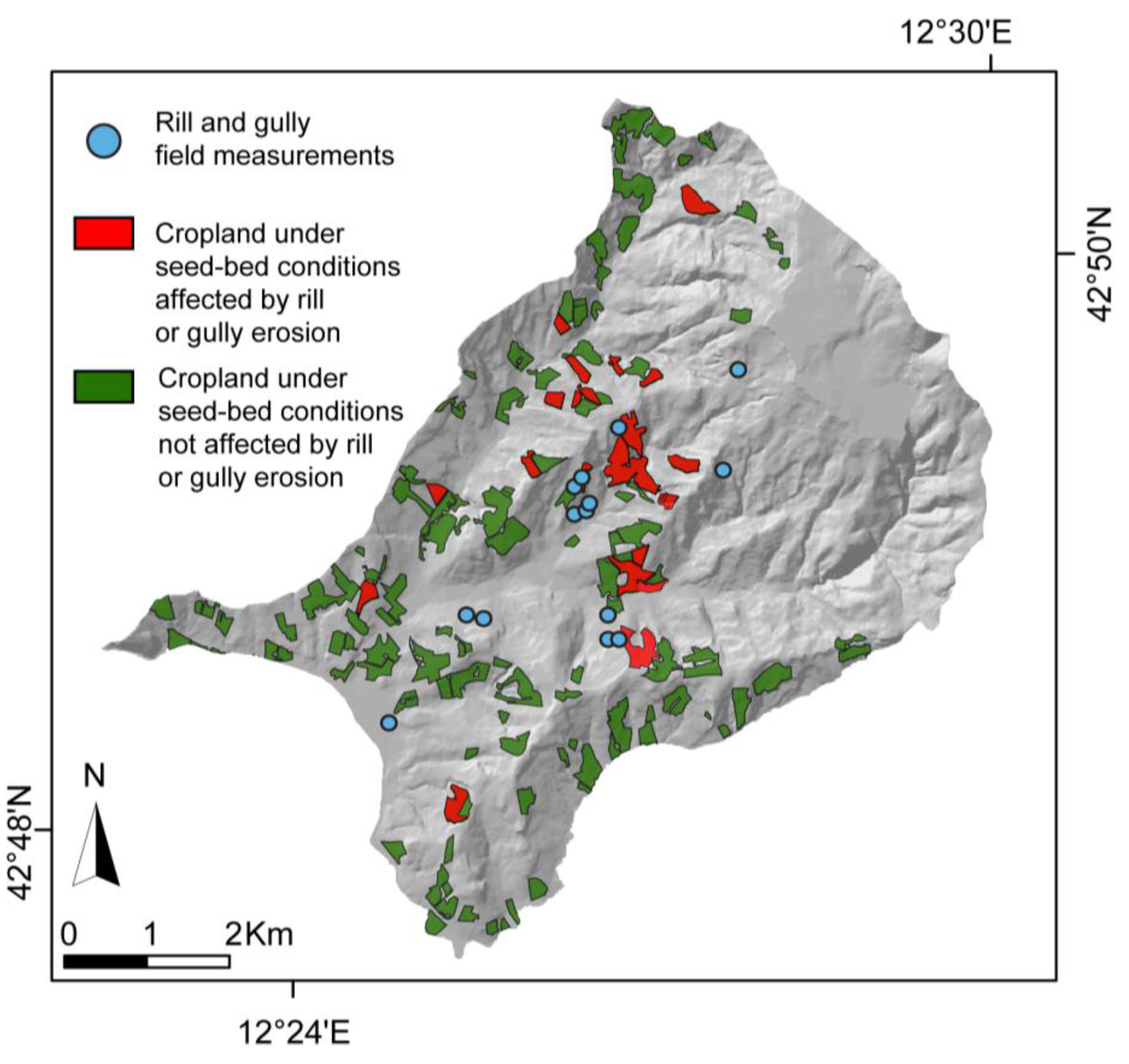
2. Study Area


3. Materials

| Date | Overlap (%) | Azimuth Angle (°) | Elevation Angle (°) | |
|---|---|---|---|---|
| WorldView-1® | 8 March 2010 | 70 | 77.30 | 57.90 |
| WorldView-1® | 8 March 2010 | 70 | 141.1 | 52.70 |
| GeoEye-1® | 27 May 2010 | 95 | 8.41 | 72.26 |
| GeoEye-1® | 27 May 2010 | 95 | 199.51 | 71.99 |
4. Methods
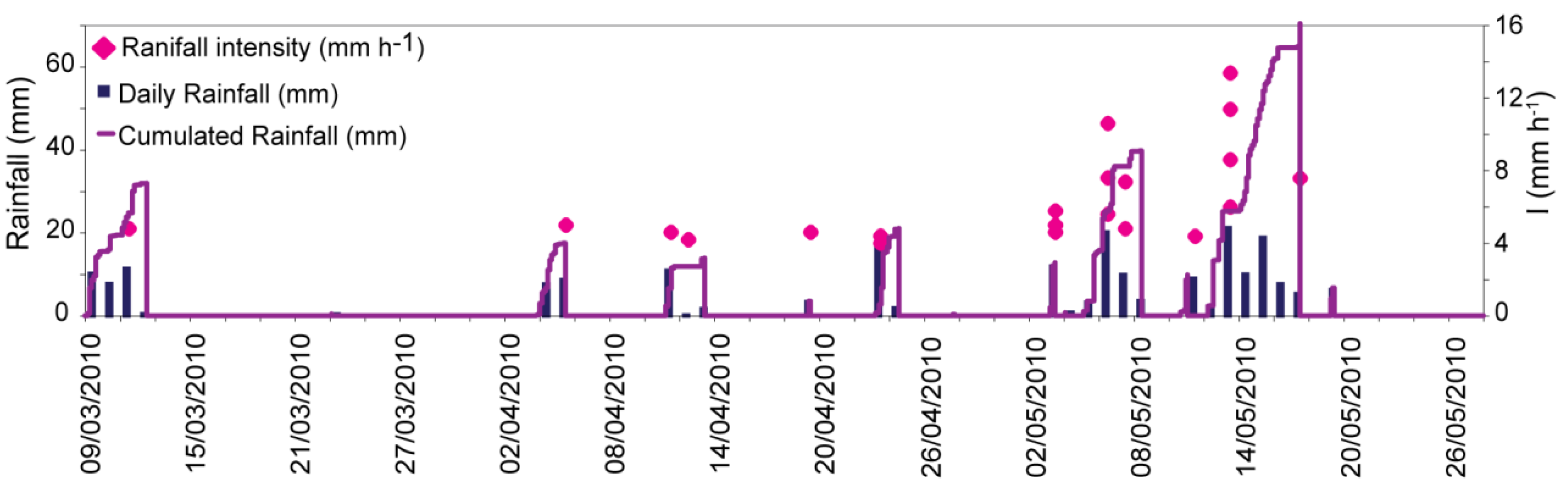
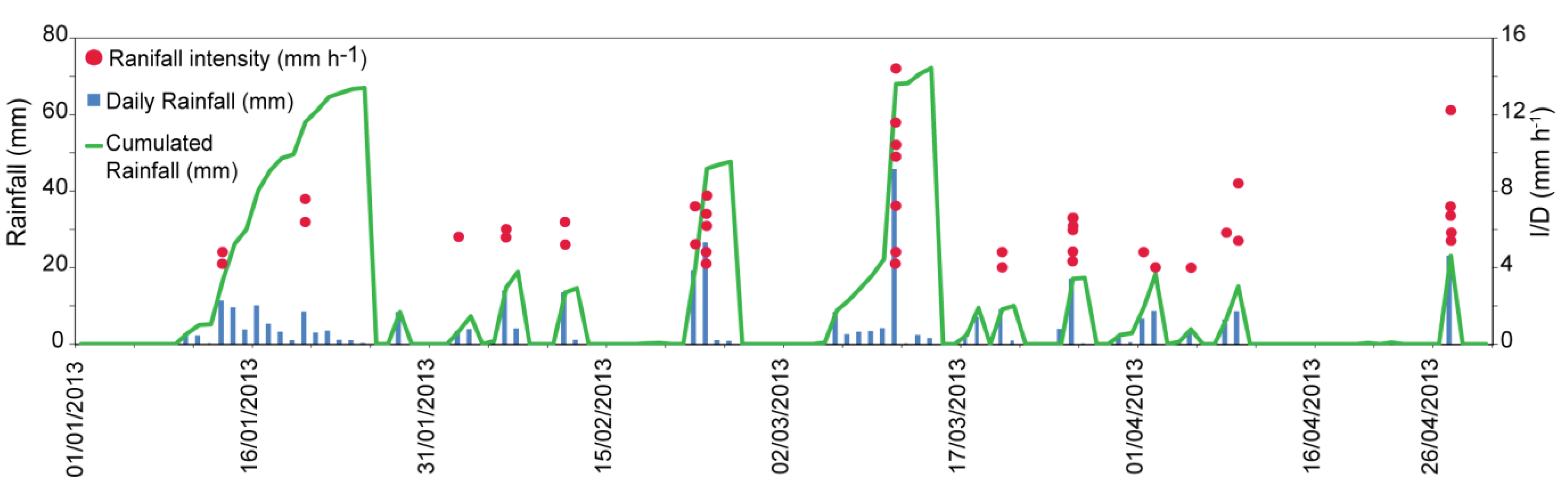
4.1. Rainfall Data and Event Reconstruction
4.2. Use of Planar’s SD StereoMirrorTM Technology

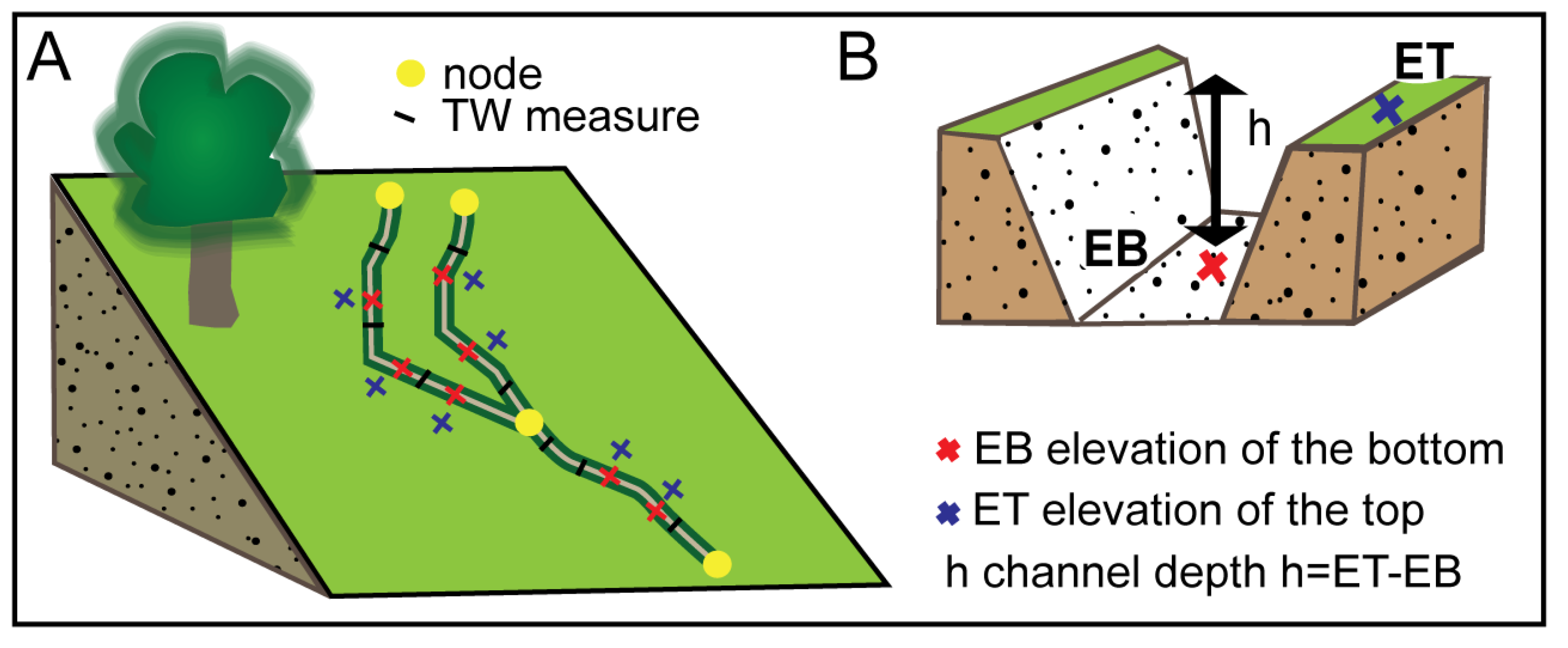
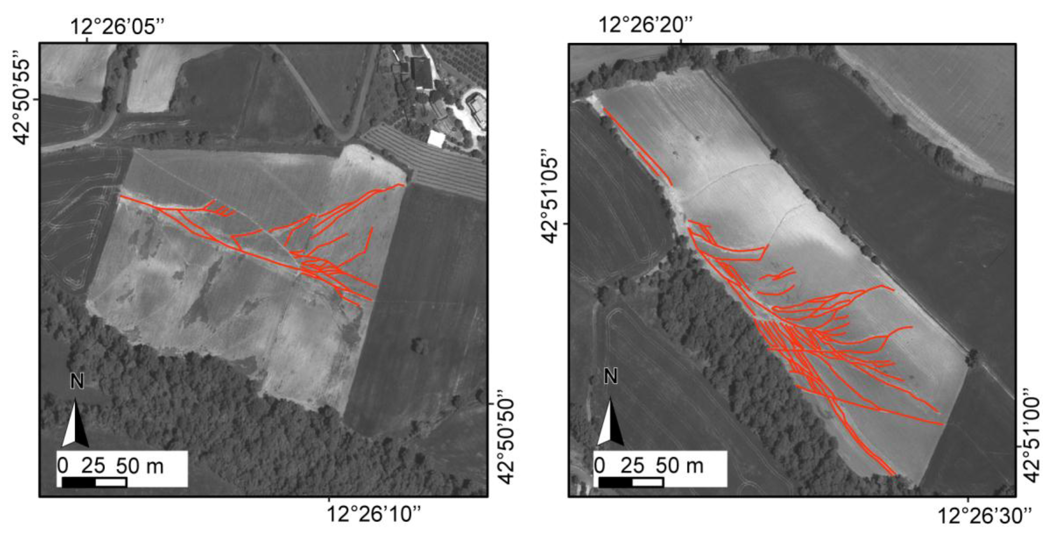
4.3. Mapping and Measuring Rills and Gullies on Satellite Stereo Images


4.3.1. Rill and Gully Volume Estimation from Satellite Measurements
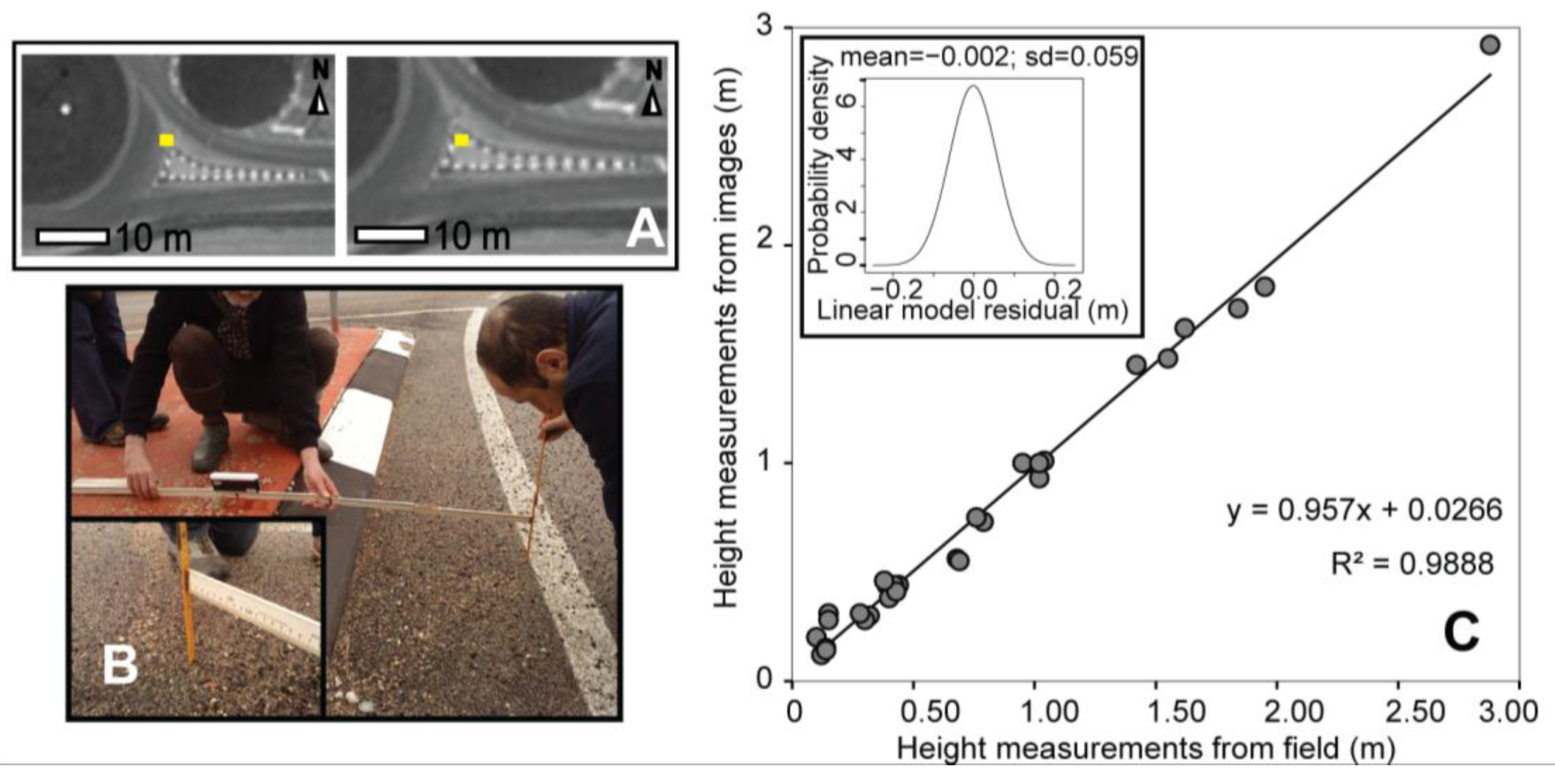
4.4. Rill and Gully Field Measurements

4.5. Channel Classification
4.6. Uncertainty of the Measurements
4.6.1. Accuracy of Satellite Height Measurements

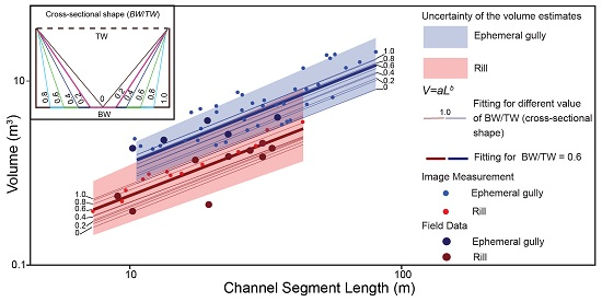
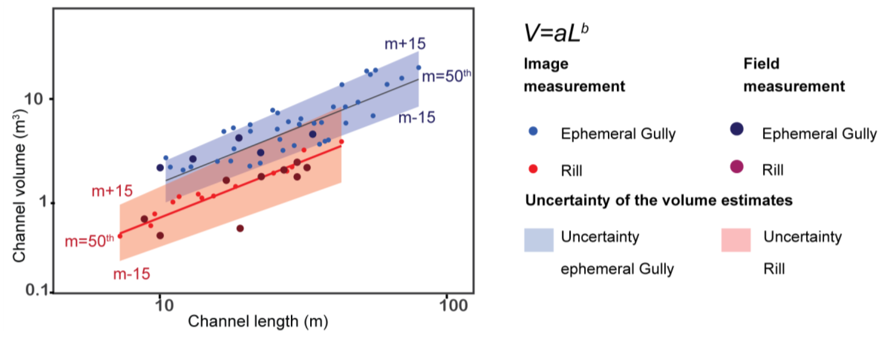
4.6.2. Volume-Length Relationship from Satellite Data and Associated Uncertainty
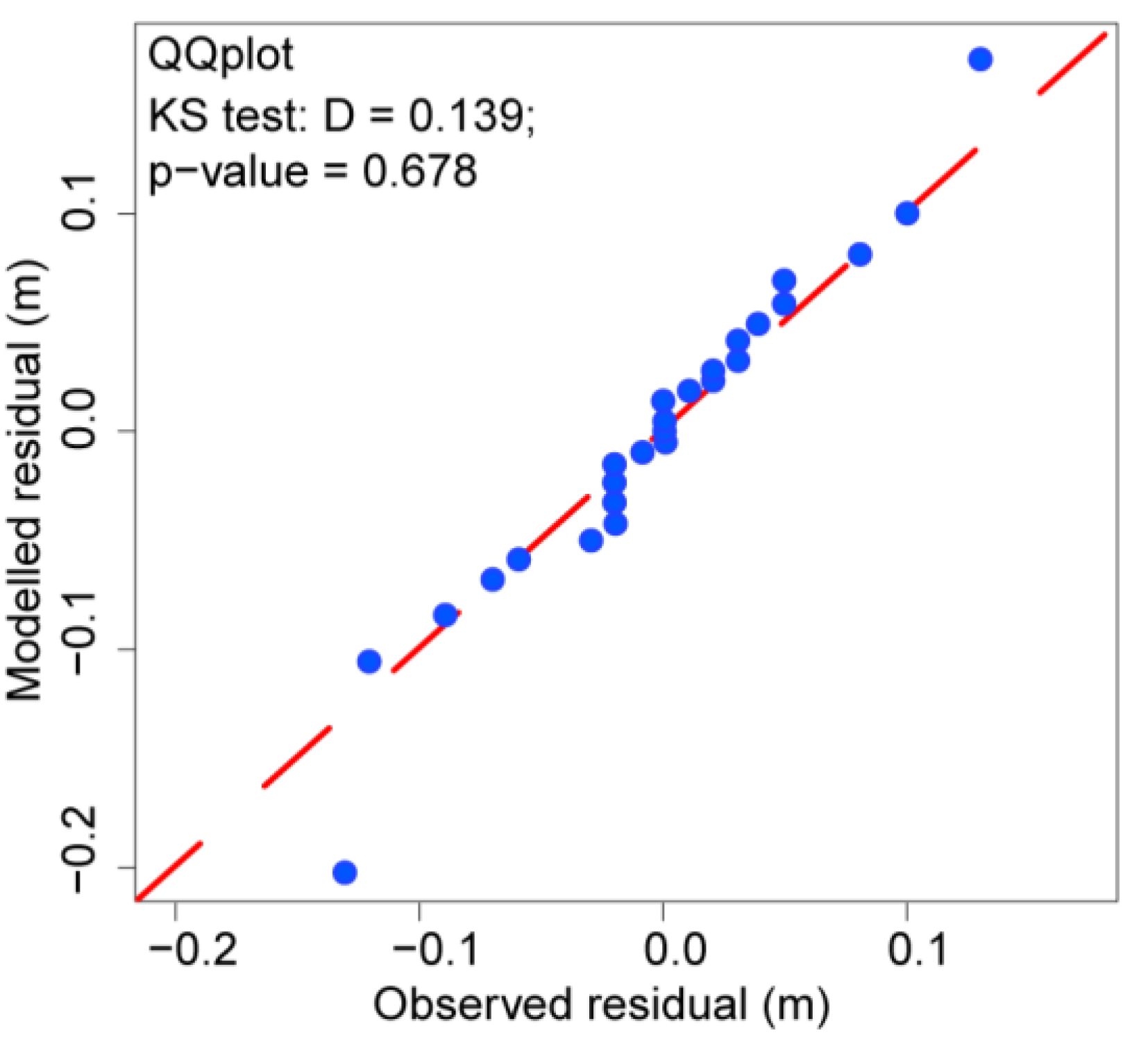
- The uncertainty that was associated with the channel depth satellite measurements (Section 5.4.1) was modelled by assuming a normal distribution for the residuals in the linear regression model.
- We used the Kolmogorov-Smirnov test (KS) and the quantile-quantile (QQ) plot of the modelled and measured errors to determine whether the normal distribution was appropriate for modeling the uncertainty that was associated with the channel depth satellite measurements.
- The normal distribution was used to generate n synthetic series of channel heights that were associated with each channel segment. Then, knowing the width and the length of the channel segments that were measured from the satellite stereo-images, we derived a synthetic series of channel volumes.
- The n synthetic series of channel volumes that were associated with the satellite channel length measurements were fitted using a least-squares approach to estimate the n power law parameters (a and b).
- The 35th and the 65th percentile values of the n power law parameters (a and b) were assumed to be representative of the uncertainty that was associated with the satellite V-L relationship estimates.
4.6.3. TW/BW Ratio and Associated Uncertainty.
4.7. Eroded Volumes and Denudation
5. Results
5.1. Rainfall Events

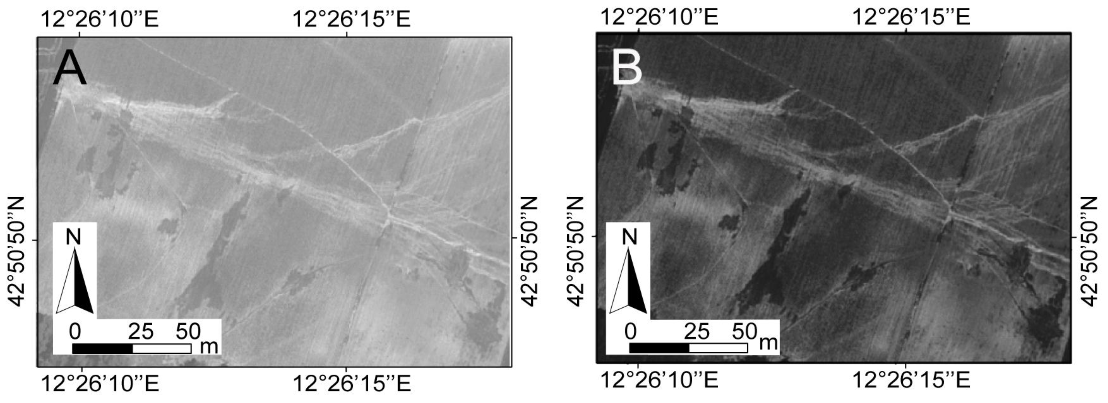
5.2. Mapping and Measuring Rills and Ephemeral Gullies on Satellite Images


| Channel # | L m | m | BW m | m | CS m2 | Volume m3 | Type |
|---|---|---|---|---|---|---|---|
| 1 | 7.34 | 0.82 | 0.49 | 0.08 | 0.05 | 0.39 | R |
| 2 | 9.40 | 0.82 | 0.49 | 0.08 | 0.05 | 0.49 | R |
| 3 | 15.56 | 0.8 | 0.48 | 0.10 | 0.06 | 1.00 | R |
| 4 | 28.03 | 0.5 | 0.30 | 0.16 | 0.06 | 1.79 | R |
| 5 | 9.70 | 1.05 | 0.63 | 0.08 | 0.07 | 0.65 | R |
| 6 | 14.17 | 1.05 | 0.63 | 0.08 | 0.07 | 0.95 | R |
| 7 | 18.57 | 1.05 | 0.63 | 0.08 | 0.07 | 1.25 | R |
| 8 | 25.17 | 0.5 | 0.30 | 0.17 | 0.07 | 1.71 | R |
| 9 | 29.18 | 0.5 | 0.30 | 0.17 | 0.07 | 1.98 | R |
| 10 | 13.76 | 1.05 | 0.63 | 0.09 | 0.08 | 1.04 | R |
| 11 | 11.23 | 1.20 | 0.72 | 0.08 | 0.08 | 0.86 | R |
| 12 | 11.79 | 1.30 | 0.78 | 0.08 | 0.08 | 0.98 | R |
| 13 | 43.43 | 1.30 | 0.78 | 0.08 | 0.08 | 3.61 | R |
| 14 | 32.15 | 0.50 | 0.30 | 0.23 | 0.09 | 2.96 | R |
| 15 | 36.42 | 1.46 | 0.87 | 0.08 | 0.09 | 3.40 | EG |
| 16 | 22.63 | 1.20 | 0.72 | 0.1 | 0.10 | 2.17 | EG |
| 17 | 38.02 | 1.50 | 0.90 | 0.08 | 0.10 | 3.65 | EG |
| 18 | 39.12 | 1.50 | 0.90 | 0.08 | 0.10 | 3.76 | EG |
| 19 | 20.81 | 0.64 | 0.38 | 0.19 | 0.10 | 2.02 | EG |
| 20 | 27.16 | 1.50 | 0.90 | 0.09 | 0.11 | 2.93 | EG |
| 21 | 29.70 | 1.73 | 1.04 | 0.08 | 0.11 | 3.29 | EG |
| 22 | 55.96 | 0.93 | 0.56 | 0.16 | 0.12 | 6.66 | EG |
| 23 | 44.99 | 0.52 | 0.31 | 0.3 | 0.12 | 5.61 | EG |
| 24 | 17.86 | 2.00 | 1.20 | 0.08 | 0.13 | 2.29 | EG |
| 25 | 16.05 | 0.8 | 0.48 | 0.22 | 0.14 | 2.26 | EG |
| 26 | 26.48 | 0.9 | 0.54 | 0.2 | 0.14 | 3.81 | EG |
| 27 | 12.18 | 1.05 | 0.63 | 0.18 | 0.15 | 1.84 | EG |
| 28 | 12.98 | 0.87 | 0.522 | 0.22 | 0.15 | 1.99 | EG |
| 29 | 37.00 | 1.2 | 0.72 | 0.16 | 0.15 | 5.68 | EG |
| 30 | 34.85 | 1.00 | 0.60 | 0.2 | 0.16 | 5.58 | EG |
| 31 | 18.34 | 2.6 | 1.56 | 0.08 | 0.17 | 3.05 | EG |
| 32 | 30.96 | 0.88 | 0.52 | 0.25 | 0.18 | 5.45 | EG |
| 33 | 11.00 | 0.90 | 0.54 | 0.25 | 0.18 | 1.98 | EG |
| 34 | 44.81 | 1.35 | 0.81 | 0.17 | 0.18 | 8.23 | EG |
| 35 | 49.58 | 0.80 | 0.48 | 0.29 | 0.19 | 9.20 | EG |
| 36 | 25.93 | 0.90 | 0.54 | 0.26 | 0.19 | 4.85 | EG |
| 37 | 31.34 | 1.24 | 0.74 | 0.2 | 0.20 | 6.22 | EG |
| 38 | 40.70 | 1.10 | 0.66 | 0.23 | 0.20 | 8.24 | EG |
| 39 | 28.35 | 1.50 | 0.90 | 0.17 | 0.20 | 5.78 | EG |
| 40 | 20.92 | 1.20 | 0.72 | 0.23 | 0.22 | 4.62 | EG |
| 41 | 62.63 | 1.40 | 0.84 | 0.2 | 0.22 | 14.03 | EG |
| 42 | 70.42 | 1.80 | 1.08 | 0.16 | 0.23 | 16.23 | EG |
| 43 | 10.61 | 1.00 | 0.6 | 0.29 | 0.23 | 2.46 | EG |
| 44 | 113.43 | 1.58 | 0.94 | 0.2 | 0.25 | 28.67 | EG |
| 45 | 80.74 | 1.54 | 0.92 | 0.21 | 0.26 | 20.89 | EG |
| 46 | 20.87 | 0.98 | 0.58 | 0.33 | 0.26 | 5.40 | EG |
| 47 | 16.90 | 1.7 | 1.02 | 0.2 | 0.27 | 4.60 | EG |
| 48 | 26.02 | 1.8 | 1.08 | 0.19 | 0.27 | 7.12 | EG |
| 49 | 18.25 | 1.56 | 0.93 | 0.22 | 0.27 | 5.01 | EG |
| 50 | 25.01 | 1.46 | 0.87 | 0.26 | 0.30 | 7.60 | EG |
| 51 | 105.80 | 1.25 | 0.75 | 0.31 | 0.31 | 32.80 | EG |
| 52 | 43.60 | 1.48 | 0.88 | 0.27 | 0.32 | 13.94 | EG |
| 53 | 54.77 | 1.50 | 0.90 | 0.27 | 0.32 | 17.74 | EG |
| 54 | 57.06 | 2.15 | 1.29 | 0.2 | 0.34 | 19.63 | EG |
| 55 | 53.16 | 1.56 | 0.93 | 0.29 | 0.36 | 19.24 | EG |
5.3. Rill and Gully Field Measurements
| Id | Type | L m | # CS | CS Average m2 | CS Max m2 | CS Min m2 | TW Max m | TW Min m | Volume m3 | Average BW/TW ratio |
|---|---|---|---|---|---|---|---|---|---|---|
| 1 | R | 47 | 20 | 0.069 | 0.11 | 0.02 | 0.90 | 0.34 | 3.32 | 0.7 |
| 2 | R | 8.8 | 7 | 0.050 | 0.08 | 0.03 | 1.20 | 0.40 | 0.55 | 0.7 |
| 3 | R | 19 | 7 | 0.069 | 0.04 | 0.01 | 0.50 | 0.34 | 0.44 | 0.5 |
| 4 | R | 30 | 8 | 0.061 | 0.10 | 0.03 | 1.00 | 0.40 | 1.50 | 0.7 |
| 5 | R | 3.2 | 2 | 0.085 | 0.09 | 0.08 | 0.50 | 0.50 | 0.30 | 0.5 |
| 6 | R | 32.5 | 7 | 0.062 | 0.14 | 0.08 | 1.30 | 0.51 | 1.88 | 0.7 |
| 7 | EG | 34 | 7 | 0.103 | 0.25 | 0.07 | 1.70 | 1.00 | 4.14 | 0.6 |
| 8 | R | 30 | 7 | 0.082 | 0.10 | 0.04 | 1.20 | 0.60 | 2.13 | 0.6 |
| 9 | EG | 22.4 | 7 | 0.144 | 0.20 | 0.09 | 1.20 | 0.48 | 2.68 | 0.7 |
| 10 | EG | 13 | 4 | 0.205 | 0.27 | 0.12 | 1.08 | 0.50 | 2.23 | 0.5 |
| 11 | R | 22.5 | 8 | 0.091 | 0.11 | 0.20 | 1.17 | 0.30 | 1.15 | 0.5 |
| 12 | EG | 18.8 | 6 | 0.250 | 0.36 | 0.16 | 1.19 | 0.77 | 3.80 | 0.3 |
| 13 | EG | 10 | 5 | 0.198 | 0.24 | 0.14 | 1.00 | 0.70 | 1.85 | 0.3 |
| Average BW/TW ratio | 0.6 | |||||||||
5.4. Measurement Uncertainty
5.4.1. Accuracy of Satellite Height Measurements
5.4.2. Volume Estimation and Associated Error


| Rill | Gully | Mixed Approach | ||||||
|---|---|---|---|---|---|---|---|---|
| Min (35th perc.) | Max (65th perc.) | Average Median | Min (35th perc.) | Max (65th perc.) | Average Median | Average Median | ||
| a | 0.027 | 0.061 | 0.044 | 0.072 | 0.101 | 0.082 | -- | |
| b | 1.04 | 1.30 | 1.20 | 1.15 | 1.24 | 1.17 | -- | |
| V (m3) | 4.62 × 10² | 2.791 × 10³ | 1.321 × 10³ | 1.844 × 10³ | 3.655 × 10³ | 2.317 × 10³ | 2.041 × 10³ | |
| Mg (γ = 1.6 Mg∙m−3) | 7.39 × 10² | 4.465 × 10³ | 2.113 × 10³ | 2.950 × 10³ | 5.848 × 10³ | 3.707 × 10³ | 3.260 × 10³ | |

5.5. Eroded Volumes and Denudation
| Catchment A = 48 km2 | Cropland Seed-Bed Condition A = 5.92 km2 | Affected Parcels A = 1.149 km2 | |||||
|---|---|---|---|---|---|---|---|
| Erosion (Mg∙ha−1) | Denudation (mm) | Erosion (Mg∙ha−1) | Denudation (mm) | Erosion (Mg∙ha−1) | Denudation (mm) | ||
| Rill | Min (35th perc.) | 0.153 | 0.010 | 1.248 | 0.078 | 6.427 | 0.402 |
| Max (65th perc.) | 0.930 | 0.0581 | 7.544 | 0.471 | 38.833 | 2.429 | |
| Average (median) | 0.440 | 0.027 | 3.571 | 0.223 | 18.382 | 1.150 | |
| Gully | Min (35th perc.) | 0.614 | 0.038 | 4.985 | 0.311 | 25.661 | 1.605 |
| Max (65th perc.) | 1.218 | 0.076 | 9.880 | 0.617 | 50.860 | 3.181 | |
| Average (median) | 0.772 | 0.048 | 6.263 | 0.391 | 32.242 | 2.017 | |
| Mixed Approach | Average (median) | 0.680 | 0.043 | 5.517 | 0.344 | 28.401 | 1.776 |
6. Discussion

| Authors | [54,56] | [55] | [56] | [57] | [58] | This Experiment |
|---|---|---|---|---|---|---|
| Study area | Spain | Belgium | Sicily(Italy) | Sicily(Italy) | Sicily(Italy) | Umbria(Italy) |
| a | 0.054 | 0.048 | 0.082 | 0.034 | 0.812 | 0.082 |
| b | 1.0.37 | 1.29 | 1.416 | 1.42 | 1..062 | 1.174 |
7. Conclusions
Acknowledgements
Author Contributions
Conflicts of Interest
References
- Poesen, J.W.A.; Torri, D.B.; Vanwalleghem, T. Gully erosion: Procedures to adopt when modelling soil erosion in landscapes affected by gullying. In Handbook of Erosion Modelling, Morgan; Morgan, R.P.C., Nearing, M.A., Eds.; John Wiley & Sons: Chichester, UK, 2010; pp. 360–386. [Google Scholar]
- Torri, D.; Borselli, L. Equation for high-rate gully erosion. Catena 2003, 50, 449–467. [Google Scholar] [CrossRef]
- Borselli, L.; Cassi, P.; Torri, D. Prolegomena to sediment and flow connectivity in the landscape: A GIS and field numerical assessment. Catena 2008, 75, 268–277. [Google Scholar] [CrossRef]
- Vigiak, O.; Newham, L.T.H.; Whitford, J.; Melland, A.; Borselli, L. Comparison of landscape approaches to define spatial patterns of hillslope-scale sediment delivery ratio. In Proceedings of 18th World IMACS/MODSIM Congress, Cairns, QLD, Australia, 13–17 July 2009.
- Nachtergaele, J.; Poesen, J. Assessment of soil losses by ephemeral gully erosion using high altitude (stereo) aerial photographs. Earth Surf. Process. Landf. 1999, 24, 693–706. [Google Scholar] [CrossRef]
- Torri, D.; Regües Muñoz, D.; Pellegrini, S.; Bazzoffi, P. Within-Storm soil surface dynamics and erosive effects of rainstorms. Catena 1999, 38, 131–150. [Google Scholar] [CrossRef]
- Bazzofi, P.; Chisci, G.; Missere, D. Influenza delle opere di livellamento e scasso sull’erosione del suolo nella collina cesenate. Riv. Agron. 1989, 23, 609–221. [Google Scholar]
- Kosov, B.F.; Kostantinova, G.S. Zoning the USSR territory by the density of gullies. Eroziia pochv i ruslovye protsessy. 1972, 4, 15–24. (In Russian) [Google Scholar]
- Nordström, K. Gully Erosion in the Lesotho Lowlands. A Geomorphological Study of the Interactions between Intrinsic and Extrinsic Variables. Ph.D. Thesis, Uppsala University, Uppsala, Sweden, 1988. [Google Scholar]
- Casalí, J.; Loizu, J.; Campo, M.A.; de Santisteban, L.M.; Alvarez-Mozos, J. Accuracy of methods for field assessment of rill and ephemeral gully erosion. Catena 2006, 67, 128–138. [Google Scholar] [CrossRef]
- Moody, J.A.; Kinner, D.A. Spatial structures of stream and hillslope drainage networks following gully erosion after wildfire. Earth Surf. Process. Landf. 2006, 31, 319–337. [Google Scholar] [CrossRef]
- Nyssen, J.; Poesen, J.; Veyret-Picot, M.; Moeyersons, J.; Haile, M.; Deckers, J.; Dewit, J.; Naudts, J.; Teka, K.; Govers, G. Assessment of gully erosion rates through interviews and measurements: a case study from northern Ethiopia. Earth Surf. Process. Landf. 2006, 31, 167–185. [Google Scholar] [CrossRef]
- Ahmadov, H.M. Gully erosion rate in Tadjikistan. Gheomorfologhia 1977, 5, 51–55. (In Russian) [Google Scholar]
- Bocco, G. Gully erosion: Processes and models. Prog. Phys. Geogr. 1991, 15, 392–406. [Google Scholar] [CrossRef]
- Burkard, M.B.; Kostaschuk, R.A. Patterns and controls of gully growth along the shoreline of Lake Huron. Earth Surf. Process. Landf. 1997, 22, 901–911. [Google Scholar] [CrossRef]
- Pellikkaa, P.K.E.; Clarka, B.J.F.; Sirviöa, T.; Masalina, K. Environmental change monitoring applying satellite and airborne remote sensing data in the Taita Hills, Kenya. In Proceedings of the 1st International Conference on Remote Sensing and Geoinformation Processing in the Assessment and Monitoring of Land Degradation and Desertification, Trier, Germany, 7–9 September 2005; pp. 223–232.
- Marzolff, I.; Poesen, J. The potential of 3D gully monitoring with GIS using high resolution aerial photography and a digital photogrammetry system. Geomorphology 2009, 111, 48–60. [Google Scholar] [CrossRef]
- Perroy, R.L.; Bookhagen, B.; Asner, G.P.; Chadwick, O.A. Comparison of gully erosion estimates using airborne and ground-based LiDAR on Santa Cruz Island, California. Geomorphology 2010, 118, 288–300. [Google Scholar] [CrossRef]
- D’Oleire-Oltmanns, S.; Marzolff, I.; Peter, K.D.; Ries, J.B. Unmanned Aerial Vehicle (UAV) for monitoring soil erosion in Morocco. Remote Sens. 2012, 4, 3390–3416. [Google Scholar] [CrossRef]
- Peter, K.D.; d’Oleire-Oltmanns, S.; Ries, J.B.; Marzolff, I.; Hssaine, A.A. Soil erosion in gully catchments affected by land-levelling measures in the Souss Basin, Morocco, analyzed by rainfall simulation and UAV remote sensing data. Catena 2014, 113, 24–40. [Google Scholar] [CrossRef]
- Kaiser, A.; Neugirg, F.; Rock, G.; Müller, C.; Haas, F.; Ries, J.; Schmidt, J. Small-Scale surface reconstruction and volume calculation of soil erosion in complex Moroccan gully morphology using structure from motion. Remote Sens. 2014, 6, 7050–7080. [Google Scholar] [CrossRef]
- Gómez-Gutiérrez, Á.; Schnabel, S.; Berenguer-Sempere, F.; Lavado-Contador, F.; Rubio-Delgado, J. Using 3D photo-reconstruction methods to estimate gully headcut erosion. Catena 2014, 120, 91–101. [Google Scholar]
- Frankl, A.; Stal, C.; Abraha, A.; Nyssen, J.; Rieke-Zapp, D.; De Wulf, A.; Poesen, J. Detailed recording of gully morphology in 3D through image-based modelling. Catena 2015, 127, 92–101. [Google Scholar] [CrossRef] [Green Version]
- Watson, A.; Evans, R.A. Comparison of estimates of soil erosion made in the field and from photographs. Soil Tillage Res. 1991, 19, 17–27. [Google Scholar] [CrossRef]
- Keech, M.A. The photogrammetric evaluation of areal and volumetric change in a gully in Zimbabwe. In Erosion, Conservation and Small Scale Farming; Hurni, H., Tato, K., Eds.; Geographica Bernensia: Bern, Switzerland, 1992; pp. 51–52. [Google Scholar]
- Price, K.P. Detection of soil erosion within pinyon-juniper woodlands using Thematic Mapper (TM) data. Remote Sens. Environ. 1993, 45, 233–248. [Google Scholar] [CrossRef]
- Pickup, G.; Nelson, J. Use of Landsat radiance parameters to distinguish soil erosion, stability, and deposition in arid Central Australia. Remote Sens. Environ. 1984, 16, 195–209. [Google Scholar] [CrossRef]
- Pickup, G.; Chewings, V.H. Forecasting patterns of soil erosion in arid lands from Landsat MSS data. Int. J. Remote Sens. 1988, 9, 69–84. [Google Scholar] [CrossRef]
- Langran, KJ. Potential for monitoring soil erosion features and soil erosion modelling components from remotely sensed data. In Proceedings of IGARSS’83, San Francisco, CA, USA, 1–4 February 1983.
- Millington, A.C.; Townshend, J.R.G. Remote sensing applications in African erosion and sedimentation studies. In Challenges in African Hydrology and Water Resources: Proceedings of the Harare Symposium; Walling, D.E., Foster, S.S.D., Wurzel, P., Eds.; IAHS Publication: Oxfordshire, UK, 1984; pp. 373–384. [Google Scholar]
- Bouaziz, M.; Wijaya, A.; Gloaguen, R. Gully erosion mapping using aster data and drainage network analysis in the main Ethiopian rift. In Proceedings of the International Geoscience and Remote Sensing Symposium (IRARSS), Cape Town, South Africa, 12–17 July 2009; pp. 113–116.
- Vrieling, A.; de Jong, S.M.; Sterk, G.; Rodrigues, S.C. Timing of erosion and satellite data: A multi-resolution approach to soil erosion risk mapping. Int. J. Appl. Earth Obs. Geoinf. 2008, 10, 267–281. [Google Scholar] [CrossRef]
- Knight, J.; Spencer, J.; Brooks, A.; Phinn, S. Large-Area, high-resolution remote sensing based mapping of alluvial gully erosion in Australia’s tropical rivers. In Proceedings of the 5th Australian Stream Management Conference: Australian Rivers, Making a Difference, Thurgoona, NSW, Australia, 21–25 May 2007; pp. 199–204.
- Shruthi, R.B.V.; Kerle, N.; Jetten, V. Object-based gully feature extraction using high resolution imagery. Geomorphology 2011, 134, 260–268. [Google Scholar] [CrossRef]
- Frankl, A.; Zwertvaegher, A.; Poesen, J.; de Dapper, M.; Nyssen, J. Transferring Google Earth observations to GIS-software: Example from gully erosion study. Int. J. Digit. Earth 2013, 6, 196–201. [Google Scholar] [CrossRef] [Green Version]
- Frankl, A.; Poesen, J.; Scholiers, N.; Jacob, M.; Haile, M.; Deckers, J.; Nyssen, J. Factors controlling the morphology and volume (V)–length (L) relations of permanent gullies in the Northern Ethiopian Highlands. Earth Surf. Process. Landf. 2013, 38, 1672–1684. [Google Scholar] [CrossRef]
- Sattar, F.; Wasson, R.; Pearson, D.; Boggs, G.; Ahmad, W.; Nawaz, M. The development of geoinformatics based framework to quantify gully erosion. In Proceedings of the International Multidisciplinary Scientific Geo-Conference & Expo, Albena Resort, Bulgaria, 20–25 June 2010; pp. 1–9.
- Conti, M.A.; Girotti, O. Il Villafranchiano nel “Lago Tiberino”, ramo sud–occidentale: schema stratigrafico e tettonico. Geol. Romana 1977, 16, 67–80. [Google Scholar]
- Servizio Geologico Nazionale Carta Geologica dell’Umbria. Map at 1:250 000 Scale. Litografia Artistica Cartografica: Firenze, Italy, 1980. (In Italian)
- Cencetti, C. Il Villafranchiano della “riva umbra” del F. Tevere: Elementi di geomorfologia e di neotettonica. Boll. Soc. Geol. Ital. 1990, 109, 337–350. (In Italian) [Google Scholar]
- Barchi, M.; Brozzetti, F.; Lavecchia, G. Analisi strutturale e geometrica dei bacini della media valle del Tevere e della valle umbra. Boll. Soc. Geol. Ital. 1991, 110, 65–76. (In Italian) [Google Scholar]
- Fiorucci, F.; Cardinali, M.; Carlà, R.; Rossi, M.; Mondini, A.C.; Santurri, L.; Ardizzone, F.; Guzzetti, F. Seasonal landslides mapping and estimation of landslide mobilisation rates using aerial and satellite images. Geomorphology 2011, 129, 59–70. [Google Scholar] [CrossRef]
- Ardizzone, F.; Fiorucci, F.; Santangelo, M.; Cardinali, M.; Mondini, A.; Rossi, M.; Reichenbach, P.; Guzzetti, F. Very-high resolution stereoscopic satellite images for landslide mapping. In Landslide Inventory and Susceptibility and Hazard Zoning; Margottini, C., Canuti, P., Sassa, K., Eds.; Springer: Berlin, Germany, 2013; pp. 95–101. [Google Scholar]
- Cardinali, M.; Ardizzone, F.; Galli, M.; Guzzetti, F.; Reichenbach, P. Landslides triggered by rapid snow melting: The December 1996–January 1997 event in Central Italy. In Proceedings of 1st Plinius Conference on Mediterranean Storms, Maratea, Italy, 14–16 October 1999; pp. 439–448.
- Rossi, M.; Kirschbaum, D.; Luciani, S.; Mondini, A.C.; Guzzetti, F. TRMM satellite rainfall estimates for landslide early warning in Italy: Preliminary results. Proc. SPIE 2012, 8523. doi: 10.1117/12.979672. Available online: http://0-dx-doi-org.brum.beds.ac.uk/10.1117/12.979672 (accessed on 20 July 2014). [Google Scholar]
- Rossi, M.; Mondini, A.C.; Luciani, S.; Kirschbaum, D.; Valigi, D.; Guzzetti, F. Probabilistic prediction of landslides induced by rainfall. In Proceedings of the second International Conference on Vulnerability and Risk Analysis and Management (ICVRAM) and the Sixth International Symposium on Uncertainty Modelling and Analysis (ISUMA), Liverpool, UK, 13–16 July 2014.
- Rossi, M.; Mondini, A.C.; Luciani, S.; Kirschbaum, D.; Valigi, D.; Guzzetti, F. A new probabilistic clustering approach for predicting rainfall induced landslides. In Proceedings of First International Workshop on Warning Criteria for Active Slides (IWWCAS), Courmayeur, Italy, 10–12 June 2013.
- Stereo Analyst for ArcGIS; ERDAS Inc.: Norcross, GA, USA, 2009.
- Planar SD2220W Stereoscopic Monitor User’s Guide. Planar Systems: Beaverton, OR, USA, 2008.
- Murillo-García, F.; Alcántara-Ayala, I.; Ardizzone, F.; Cardinali, M.; Fiorucci, F.; Guzzetti, F. Satellite stereoscopic pair images of very high resolution: A step forward for the development of landslide inventories. Landslides 2014, 12, 1–15. [Google Scholar]
- Shaker, A.; Yan, W.Y.; Easa, S.M. Using stereo satellite imagery for topographic and transportation applications: An accuracy assessment. GISci. Remote Sens. 2010, 47, 321–337. [Google Scholar] [CrossRef]
- Hauge, C. Soil erosion definitions. California Geol. 1977, 30, 202–203. [Google Scholar]
- Poesen, J. Gully typology and gully control measures in the European loess belt. In Proceedings of International Symposium on Farm Land Erosion in Temperate Plains Environment and Hills, Paris, France, 25–29 May 1992; pp. 221–239.
- Casalí, J.; Lopez, J.J.; Giràldez, J.V. Ephemeral gully erosion in southern Navarra (Spain). Catena 1999, 36, 65–84. [Google Scholar] [CrossRef]
- Nachtergaele, J.; Poesen, J.; Steegen, A.; Takken, I.; Beuselinck, L.; Vandekerckhove, L.; Govers, G. The value of a physically based model versus an empirical approach in the prediction of ephemeral gully erosion for loess-derived soils. Geomorphology 2001, 40, 237–252. [Google Scholar] [CrossRef]
- Capra, A.; Mazzara, LM.; Scicolone, B. Application of the EGEM model to predict ephemeral gully erosion in Sicily (Italy). Catena 2005, 59, 133–146. [Google Scholar] [CrossRef]
- Capra, A.; Di Stefano, C.; Ferro, V.; Scicolone, B. Similarity between morphological characteristics of rills and ephemeral gullies in Sicily, Italy. Hydrol. Process. 2009, 23, 3334–3341. [Google Scholar] [CrossRef]
- Di Stefano, C.; Ferro, V. Measurements of rill and gully erosion in Sicily. Hydrol. Process. 2011, 25, 2221–2227. [Google Scholar] [CrossRef]
- Efron, B. Bootstrap methods: Another look to the Jackknife. Ann. Stat. 1979, 7, 1–26. [Google Scholar] [CrossRef]
- Efron, B.; Tibshirani, R.J. An Introduction to the Bootstrap; Chapman and Hall: London, UK, 1993. [Google Scholar]
- R Core Team. A language and environment for statistical computing. R Foundation for Statistical Computing: Vienna, Austria, 2015. [Google Scholar]
- Baccarini, L. Suscettibilità da frana nell’area di Collazzone (Umbria. Italia Centrale): applicazione di un modello distribuito fisicamente basato per scivolamenti profondi. Master’s Thesis, Perugia University, Perugia, Italy, 2013. [Google Scholar]
- Desprats, J.F.; Raclot, D.; Rousseau, M.; Cerdan, O.; Garcin, M.; Le Bissonnais, Y.; Ben Slimane, A.; Fouche, J.; Monfort-Climent, D. Mapping linear erosion features using high and very high resolution satellite imagery. Land Degrad. Dev. 2013, 24, 22–32. [Google Scholar] [CrossRef]
- Stöcker, C.; Eltner, A.; Karrasch, P. Measuring gullies by synergetic application of UAV and close range photogrammetry—A case study from Andalusia, Spain. Catena 2015, 132, 1–11. [Google Scholar] [CrossRef]
- Torri, D.; Borselli, L.; Guzzetti, F.; Calzolari, M.C.; Bazzoffi, P.; Ungaro, F.; Bartolini, D.; Salvador Sanchis, M.P. Italy. In Soil Erosion in Europe; Poesen, J., Boardman, J., Eds.; John Willey & Son: West Sussex, UK, 2006; pp. 245–261. [Google Scholar]
- Young, A. Present rate of land erosion. Nature 1969, 224, 851–852. [Google Scholar] [CrossRef]
- Alexandrovskiy, A.L. Rates of soil-forming processes in three main models of pedogenesis. In Rev. Mex. Cienc. Geol.; 2007; Volume 24, pp. 283–292. [Google Scholar]
- Poesen, J.; Nachtergaele, J.; Verstraeten, G.; Valentin, C. Gully erosion and environmental change: Importance and research needs. Catena 2003, 50, 91–133. [Google Scholar] [CrossRef]
- Poesen, J.; Vandekerckhove, L.; Nachtergaele, J.; Oostwoud Wijdenes, D.; Verstraeten, G.; van Wesemael, B. Gully erosion in dryland environments. In Dryland Rivers: Hydrology and Geomorphology of Semi-Arid Channels; Bull, L.J., Kirkby, M.J., Eds.; Wiley: Chichester, UK, 2002; pp. 229–262. [Google Scholar]
- Aucelli, P.P.C.; Conforti, M.; Della Seta, M.; Del Monte, M.; D’uva, L.; Rosskopf, C.M.; Vergari, F. Multi temporal digital photogrammetric analysis for quantitative assessment of soil erosion rates in the Landola catchment of the Upper Orcia Valley (Tuscany, Italy). Land Degrad. Dev. 2014. doi: 10.1002/ldr.2324. Available online: http://0-onlinelibrary-wiley-com.brum.beds.ac.uk/doi/10.1002/ldr.2324/epdf (accessed on 5 October 2014). [Google Scholar]
- Della Seta, M.; del Monte, M.; Fredi, P.; Lupia Palmieri, E. Direct and indirect evaluation of denudation rates in Central Italy. Catena 2007, 71, 21–30. [Google Scholar] [CrossRef]
- Giménez, R.; Marzolff, I.; Campo, M.A.; Seeger, M.; Ries, J.B.; Casalí, J.; Álvarez-Mozos, J. Accuracy of high-resolution photogrammetric measurements of gullies with contrasting morphology. Earth Surf. Process. Landf. 2009, 34, 1915–1926. [Google Scholar] [CrossRef]
© 2015 by the authors; licensee MDPI, Basel, Switzerland. This article is an open access article distributed under the terms and conditions of the Creative Commons Attribution license (http://creativecommons.org/licenses/by/4.0/).
Share and Cite
Fiorucci, F.; Ardizzone, F.; Rossi, M.; Torri, D. The Use of Stereoscopic Satellite Images to Map Rills and Ephemeral Gullies. Remote Sens. 2015, 7, 14151-14178. https://0-doi-org.brum.beds.ac.uk/10.3390/rs71014151
Fiorucci F, Ardizzone F, Rossi M, Torri D. The Use of Stereoscopic Satellite Images to Map Rills and Ephemeral Gullies. Remote Sensing. 2015; 7(10):14151-14178. https://0-doi-org.brum.beds.ac.uk/10.3390/rs71014151
Chicago/Turabian StyleFiorucci, Federica, Francesca Ardizzone, Mauro Rossi, and Dino Torri. 2015. "The Use of Stereoscopic Satellite Images to Map Rills and Ephemeral Gullies" Remote Sensing 7, no. 10: 14151-14178. https://0-doi-org.brum.beds.ac.uk/10.3390/rs71014151