
Derivation of High-Resolution Bathymetry from Multispectral Satellite Imagery: A Comparison of Empirical and Optimisation Methods through Geographical Error Analysis

Abstract
:1. Introduction

| Bathymetric Mapping Development | Reference |
|---|---|
| “Depth of penetration” zones mapped from the range of depths to which light penetrates through the water column at different wavelengths. | Jupp, 1988 [16] |
| Pair-wise waveband correction of absorption and scattering in the water column to derive a single depth-invariant index. Light transfer is assumed to decrease exponentially with vertical depth. | Lyzenga, 1978; 1981 [7,17] |
| A semi-analytical model developed for shallow water remote sensing based on radiative transfer. | Lee et al., 1998 [18] |
| An inversion optimisation approach developed to simultaneously derive water depth and water column properties from hyper-spectral data. | Lee et al., 1999 [19] |
| Empirically deriving the relationship between the changing ratio of two water-penetrating waveband pairs and water depth, independently of bottom albedo. | Stumpf et al., 2003 [8] |
| Linear regression of reflectance principal components, with uniform bottom types | Mishra et al., 2004 [20] |
| A semi-analytical model similar to that of Lee et al. [18] incorporating the assumption of constant water optical properties across the scene. | Adler-Golden et al., 2005 [21] |
| A semi-analytical model similar to that of Lee et al. [18] that included a quantitative comparison of model-derived depth with high-resolution multi-beam acoustic bathymetry data. | Mcintyre et al., 2006 [22] |
| Linear unmixing of the benthic cover incorporated into semi-analytical approaches. | Goodman and Ustin, 2007 [23], Klonowski et al., 2007 [10] |
| Lookup table approach for matching image spectra to a library of spectra corresponding to different combinations of depth, bottom type and water properties. | Louchard et al., 2003 [24], Mobley et al., 2005 [9], Lesser and Mobley, 2007 [25] Hedley et al., 2009 [26] |
| A bio-optical optimization model for simultaneous retrieval of the optical properties of the water column and bottom from remotely-sensed imagery in optically-deep and optically-shallow waters. | Giardino et al., 2012 [27] |
| An assessment of Sentinel-2, a moderate resolution, multispectral satellite sensor for bathymetric mapping, including the propagation of noise and environmental uncertainties through a radiative transfer model inversion to quantify uncertainty in the retrievable parameters. | Hedley et al., 2012 [28] |
2. Methods
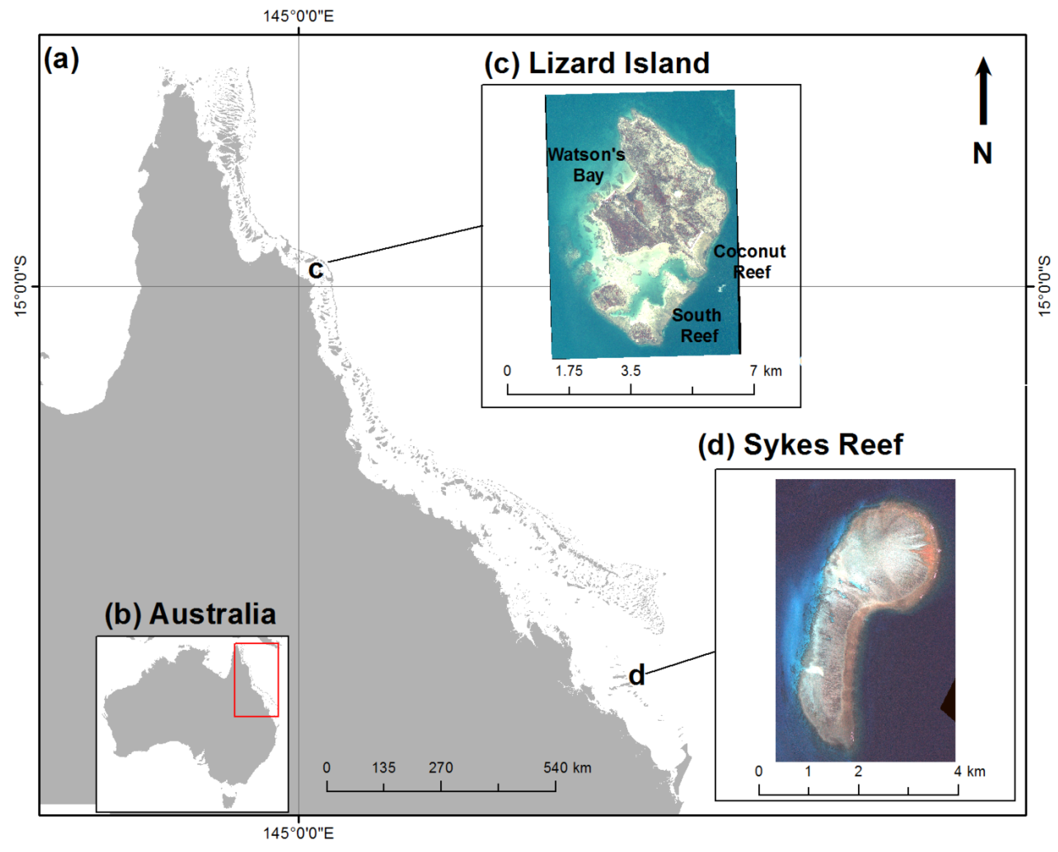
2.1. Site Locations

2.2. Collection of in situ Bathymetric Measurements

2.3. Image Pre-Processing: Atmospheric and Glint Correction
| Lizard Island WorldView-2 Image | Sykes Reef Worldview-2 Image | |
|---|---|---|
| Acquisition date | 10 October 2011 | 14 February 2014 |
| Tidal stage | Mean sea level, rising flood | Mean sea level, rising flood |
| Weather conditions | Low cloud, calm | Low cloud, calm |
2.4. Bathymetric Mapping: Empirical Approach
2.5. Bathymetric Mapping: Optimisation Approach
2.6. Mapping Model Residuals
2.7. Statistical Exploration of Model Residuals: Independent Validation Plots, Moran’s I
2.8. Modelling the Spatially-Structured Component Error Component
3. Results
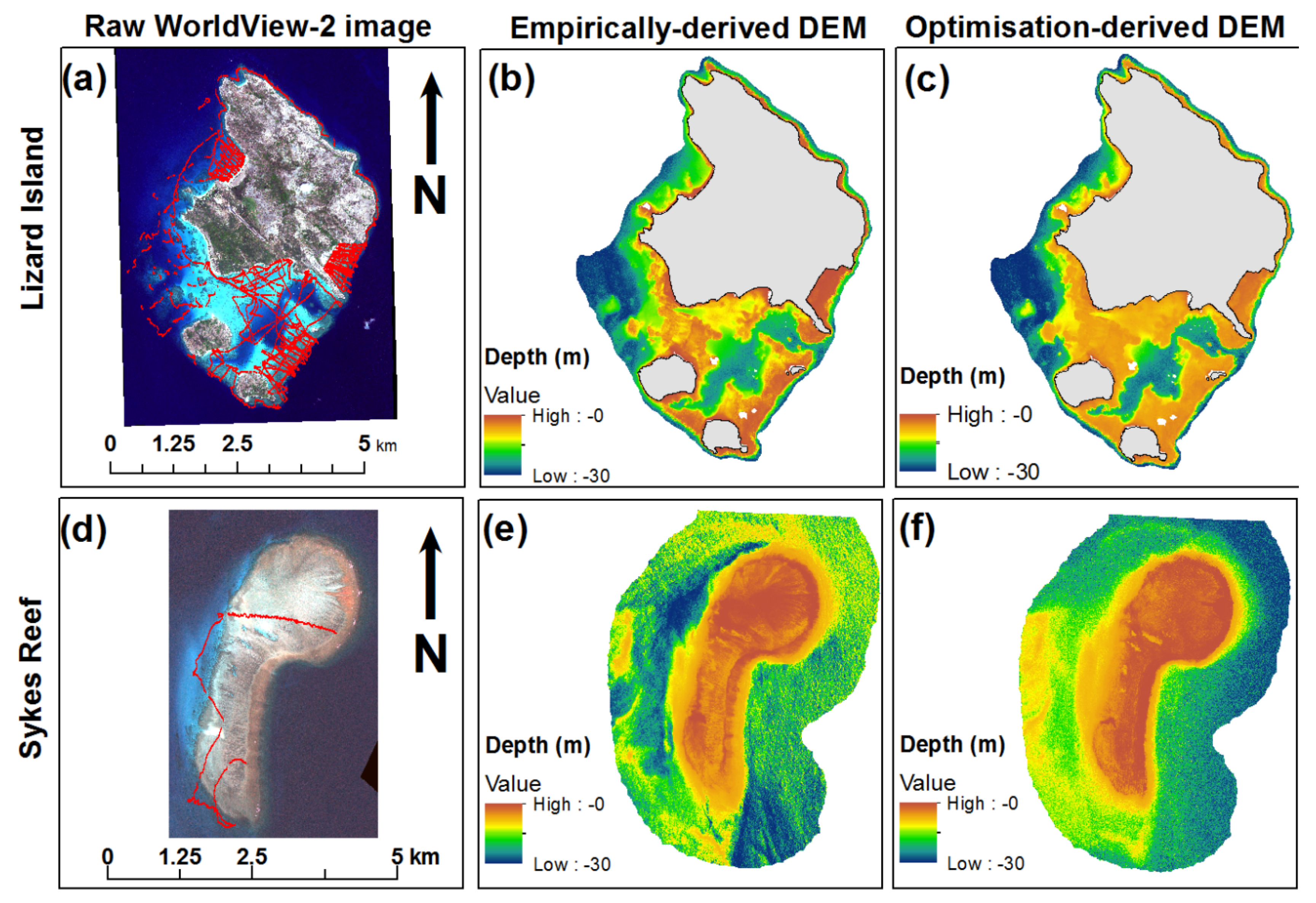
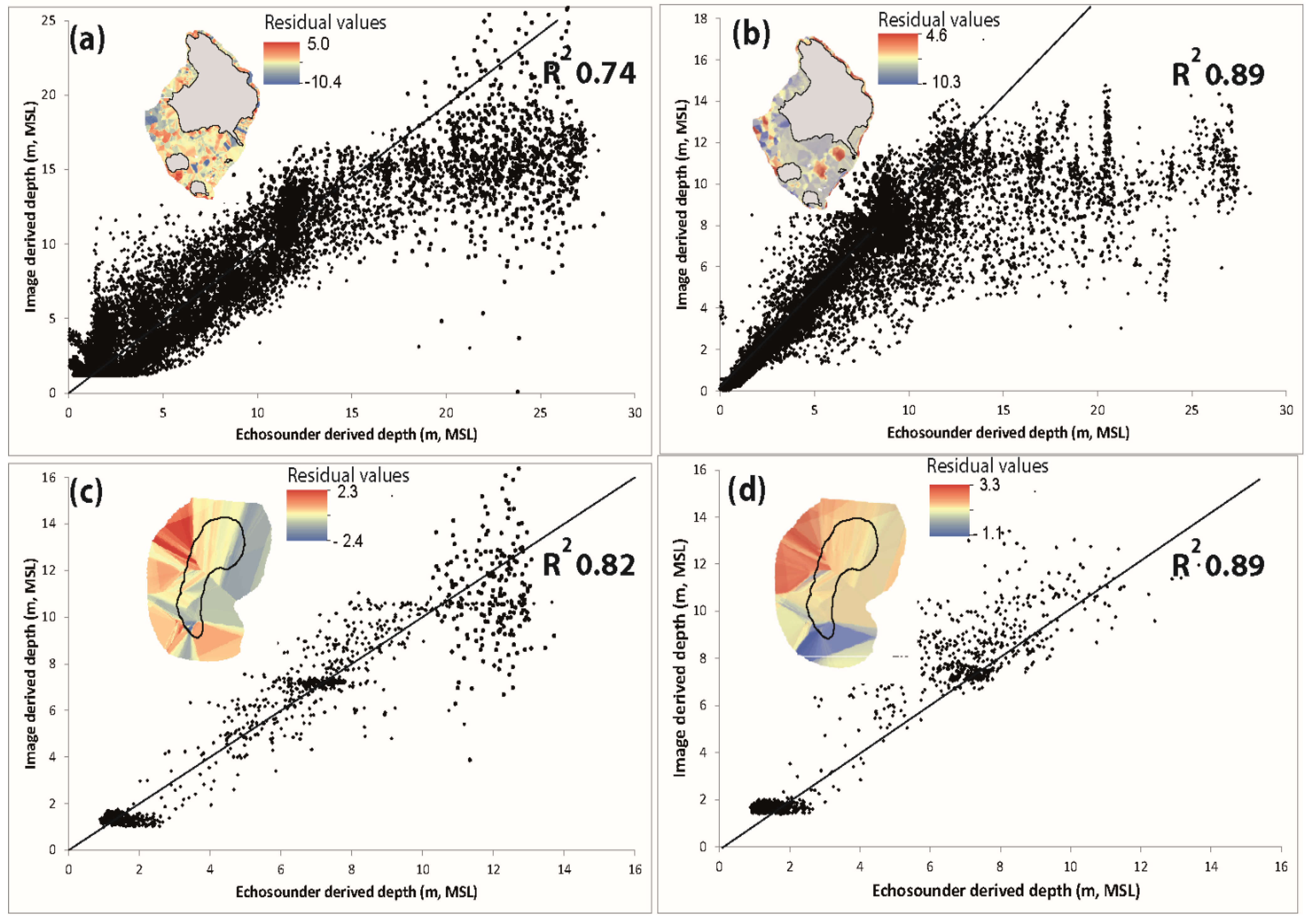
3.1. Bathymetric Mapping
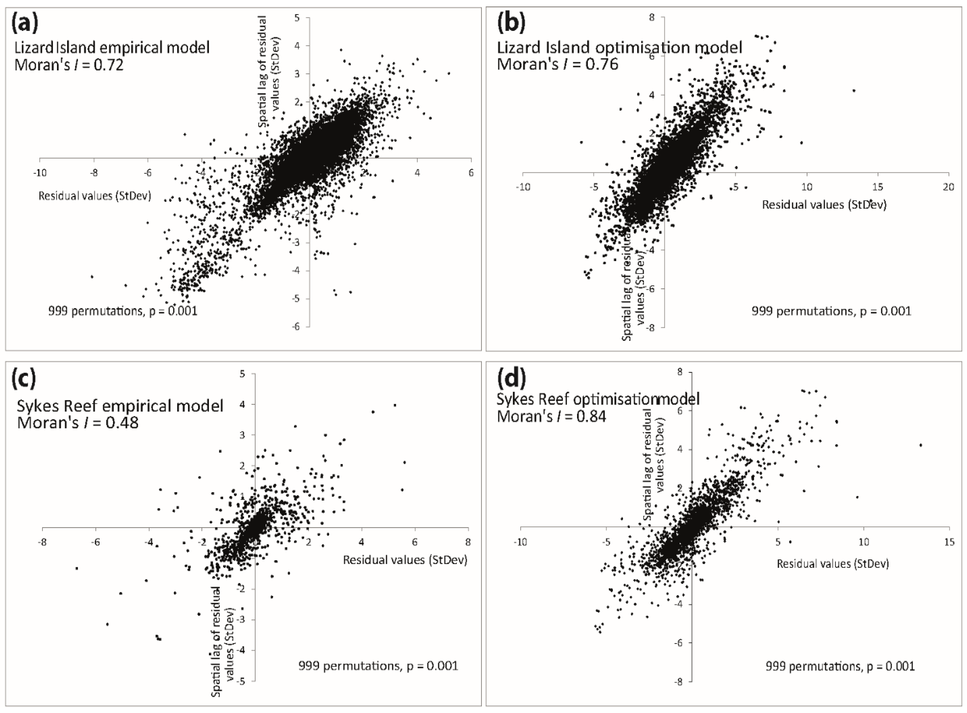
3.2. Exploration of Model Residuals: Mapping Model Residuals and Exploring Moran’s I


3.3. Modelling the Spatially-Structured Error Component
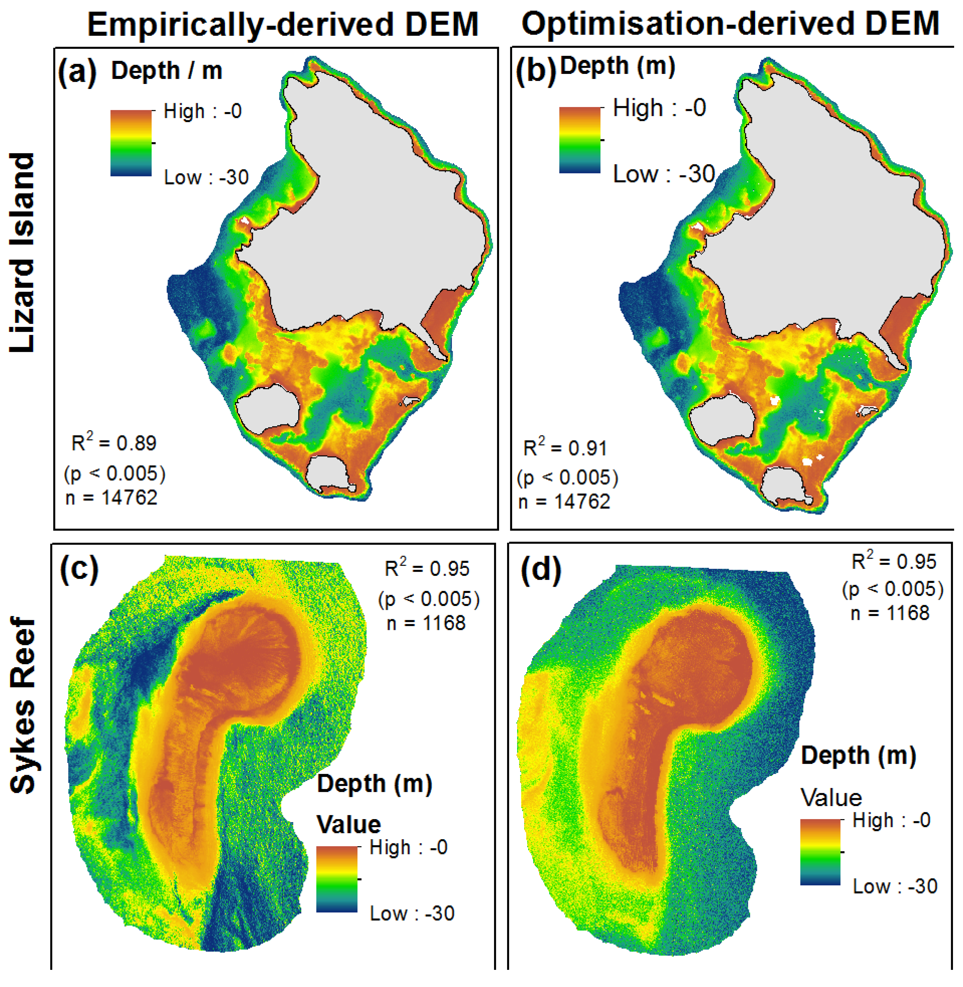
| n | Standard Model R2 | Spatial Error Model R2 | |
|---|---|---|---|
| Lizard Island empirical bathymetry estimates. | 14,762 | 0.74 | 0.89 |
| Lizard Island optimisation bathymetry estimates. | 14,762 | 0.89 | 0.91 |
| Sykes Reef empirical bathymetry estimates. | 1168 | 0.82 | 0.95 |
| Sykes Reef optimisation bathymetry estimates. | 1168 | 0.89 | 0.95 |

4. Discussion
5. Conclusions
Acknowledgments
Author Contributions
Conflicts of Interest
References
- Hubbard, D. Reefs as dynamic systems. In Life and Death of Coral Reefs; Birkeland, C., Ed.; Chapman & Hall: New York, NY, USA, 1997; pp. 43–67. [Google Scholar]
- Kleypas, J.A.; McManus, J.W.; Meñez, L.A. Environmental limits to coral reef development: Where do we draw the line? Am. Zool. 1999, 39, 146–159. [Google Scholar] [CrossRef]
- Brown, C.J.; Smith, S.J.; Lawton, P.; Anderson, J.T. Benthic habitat mapping: A review of progress towards improved understanding of the spatial ecology of the seafloor using acoustic techniques. Estuar., Coastal Shelf Sci. 2011, 92, 502–520. [Google Scholar] [CrossRef]
- Arias-González, J.E.; Acosta-González, G.; Membrillo, N.; Garza-Pérez, J.R.; Castro-Pérez, J.M. Predicting spatially explicit coral reef fish abundance, richness and Shannon-Weaver index from habitat characteristics. Biodivers. Conserv. 2012, 21, 115–130. [Google Scholar] [CrossRef]
- Harborne, A.R.; Mumby, P.J.; Ferrari, R. The effectiveness of different meso-scale rugosity metrics for predicting intra-habitat variation in coral-reef fish assemblages. Environ. Biol. Fish. 2012, 94, 431–442. [Google Scholar] [CrossRef]
- Dekker, A.G.; Phinn, S.R.; Anstee, J.; Bissett, P.; Brando, V.E.; Casey, B.; Fearns, P.; Hedley, J.; Klonowski, W.; Lee, Z.P. Intercomparison of shallow water bathymetry, hydro‐optics, and benthos mapping techniques in australian and caribbean coastal environments. Limnol. Oceanogr. Meth. 2011, 9, 396–425. [Google Scholar] [CrossRef]
- Lyzenga, D.R. Remote sensing of bottom reflectance and water attenuation parameters in shallow water using aircraft and landsat data. Int. J. Remote Sens. 1981, 2, 71–82. [Google Scholar] [CrossRef]
- Stumpf, R.P.; Holderied, K.; Sinclair, M. Determination of water depth with high‐resolution satellite imagery over variable bottom types. Limnol. Oceanogr. 2003, 48, 547–556. [Google Scholar] [CrossRef]
- Mobley, C.D.; Sundman, L.K.; Davis, C.O.; Bowles, J.H.; Downes, T.V.; Leathers, R.A.; Montes, M.J.; Bissett, W.P.; Kohler, D.D.; Reid, R.P. Interpretation of hyperspectral remote-sensing imagery by spectrum matching and look-up tables. Appl. Opt. 2005, 44, 3576–3592. [Google Scholar] [CrossRef] [PubMed]
- Klonowski, W.M.; Fearns, P.R.; Lynch, M.J. Retrieving key benthic cover types and bathymetry from hyperspectral imagery. J. Appl. Remote Sens. 2007, 1, 011505. [Google Scholar] [CrossRef]
- Haining, R.P. Spatial Data Analysis; Cambridge University Press: Cambridge, UK, 2003. [Google Scholar]
- Upton, G.; Fingleton, B. Spatial Data Analysis by Example. Volume 1: Point Pattern and Quantitative Data; John Wiley & Sons Ltd.: Chichester, UK, 1985. [Google Scholar]
- Fotheringham, S.; Rogerson, P. Spatial Analysis and Gis; CRC Press: Boca Raton, FL, USA, 2013. [Google Scholar]
- Tukey, J.W. Exploratory data analysis. Read. Ma 1977. [Google Scholar] [CrossRef]
- Tobler, W.R. A computer movie simulating urban growth in the detroit region. Econ. Geogr. 1970, 46, 234–240. [Google Scholar] [CrossRef]
- Jupp, D. Background and extensions to depth of penetration (dop) mapping in shallow coastal waters. In Proceedings of 1988 Remote Sensing of the Coastal Zone International Symposium, Queensland, Australia, 7–9 September 1988.
- Lyzenga, D.R. Passive remote sensing techniques for mapping water depth and bottom features. Appl. Opt. 1978, 17, 379–383. [Google Scholar] [CrossRef] [PubMed]
- Lee, Z.; Carder, K.L.; Mobley, C.D.; Steward, R.G.; Patch, J.S. Hyperspectral remote sensing for shallow waters. I. A semianalytical model. Appl. Opt. 1998, 37, 6329–6338. [Google Scholar] [PubMed]
- Lee, Z.; Carder, K.L.; Mobley, C.D.; Steward, R.G.; Patch, J.S. Hyperspectral remote sensing for shallow waters: 2. Deriving bottom depths and water properties by optimization. Appl. Opt. 1999, 38, 3831–3843. [Google Scholar] [CrossRef] [PubMed]
- Mishra, D.; Narumalani, S.; Lawson, M.; Rundquist, D. Bathymetric mapping using ikonos multispectral data. GISci. Remote Sens. 2004, 41, 301–321. [Google Scholar] [CrossRef]
- Adler-Golden, S.M.; Acharya, P.K.; Berk, A.; Matthew, M.W.; Gorodetzky, D. Remote bathymetry of the littoral zone from aviris, lash, and quickbird imagery. IEEE Trans. Geosci. Remote Sens 2005, 43, 337–347. [Google Scholar] [CrossRef]
- McIntyre, M.L.; Naar, D.F.; Carder, K.L.; Donahue, B.T.; Mallinson, D.J. Coastal bathymetry from hyperspectral remote sensing data: Comparisons with high resolution multibeam bathymetry. Mar. Geophys. Res. 2006, 27, 129–136. [Google Scholar] [CrossRef]
- Goodman, J.; Ustin, S.L. Classification of benthic composition in a coral reef environment using spectral unmixing. J. Appl. Remote Sens. 2007, 1, 011501. [Google Scholar]
- Louchard, E.M.; Reid, R.P.; Stephens, F.C.; Davis, C.O.; Leathers, R.A.; T Valerie, D. Optical remote sensing of benthic habitats and bathymetry in coastal environments at lee stocking island, bahamas: A comparative spectral classification approach. Limnol. Oceanogr. 2003, 48, 511–521. [Google Scholar] [CrossRef]
- Lesser, M.; Mobley, C. Bathymetry, water optical properties, and benthic classification of coral reefs using hyperspectral remote sensing imagery. Coral Reefs 2007, 26, 819–829. [Google Scholar] [CrossRef]
- Hedley, J.; Roelfsema, C.; Phinn, S.R. Efficient radiative transfer model inversion for remote sensing applications. Remote Sens. Environ. 2009, 113, 2527–2532. [Google Scholar] [CrossRef]
- Giardino, C.; Candiani, G.; Bresciani, M.; Lee, Z.; Gagliano, S.; Pepe, M. Bomber: A tool for estimating water quality and bottom properties from remote sensing images. Comput. Geosci. 2012, 45, 313–318. [Google Scholar] [CrossRef]
- Hedley, J.; Roelfsema, C.; Koetz, B.; Phinn, S. Capability of the sentinel 2 mission for tropical coral reef mapping and coral bleaching detection. Remote Sens. Environ. 2012, 120, 145–155. [Google Scholar] [CrossRef]
- Rees, S.A.; Opdyke, B.N.; Wilson, P.A.; Fifield, L.K.; Levchenko, V. Holocene evolution of the granite based lizard island and macgillivray reef systems, northern great barrier reef. Coral Reefs 2006, 25, 555–565. [Google Scholar] [CrossRef]
- Maxwell, W. Atlas of the Great Barrier Reef; Elsevier: Amsterdam, NY, USA, 1968. [Google Scholar]
- Jell, J.S.; Flood, P.G. Guide to the Geology of Reefs of the Capricorn and Bunker Groups, Great Barrier Reef Province, with Special Reference to Heron Reef; University of Queensland Press: Brisbane, Australia, 1978. [Google Scholar]
- Marshall, J.F.; Davies, P.J. Submarine lithification on windward reef slopes: Capricorn-bunker group, southern great barrier reef. J. Sediment. Res. 1981, 51, 953–960. [Google Scholar]
- Davies, P.; Marshall, J.; Hekel, H.; Searle, D. Shallow inter-reefal structure of the capricorn group, southern great barrier reef. BMR J. Aust. Geol. Geophys. 1981, 6, 101–105. [Google Scholar]
- Wells, D.E.; Monahan, D. Iho s44 standards for hydrographic surveys and the variety of requirements for bathymetric data. Hydrogr. J. 2002, 44, 9–16. [Google Scholar]
- Antoine, D.; Morel, A. A multiple scattering algorithm for atmospheric correction of remotely sensed ocean colour (meris instrument): Principle and implementation for atmospheres carrying various aerosols including absorbing ones. Int. J. Remote Sens. 1999, 20, 1875–1916. [Google Scholar] [CrossRef]
- Mayer, B.A.; Kylling, A. The libradtran software package for radiative transfer calculations-description and examples of use. Atmos. Chem. Phys. 2005, 5, 1855–1877. [Google Scholar] [CrossRef]
- Hedley, J.; Harborne, A.; Mumby, P. Simple and robust removal of sun glint for mapping shallow‐water benthos. Int. J. Remote Sens 2005, 26, 2107–2112. [Google Scholar] [CrossRef]
- Hedley, J.D.; Roelfsema, C.M.; Phinn, S.R.; Mumby, P.J. Environmental and sensor limitations in optical remote sensing of coral reefs: Implications for monitoring and sensor design. Remote Sens. 2012, 4, 271–302. [Google Scholar] [CrossRef]
- Hedley, J.; Roelfsema, C.; Phinn, S. Propogating uncertainty through a shallow water mapping algorithm based on radiative transfer model inversion. Ocean Opt. 2010, 12, 24–51. [Google Scholar]
- Franklin, J. Mapping Species Distributions: Spatial Inference and Prediction; Cambridge University Press: Cambridge, UK, 2010. [Google Scholar]
- Kyriakidis, P.C.; Dungan, J.L. A geostatistical approach for mapping thematic classification accuracy and evaluating the impact of inaccurate spatial data on ecological model predictions. Environ. Ecol. Stat. 2001, 8, 311–330. [Google Scholar] [CrossRef]
- Anselin, L.; Bera, A.K. Spatial dependence in linear regression models with an introduction to spatial econometrics. Stat. Textb. Monogr. 1998, 155, 237–290. [Google Scholar]
- Leon, J.X.; Phinn, S.R.; Hamylton, S.; Saunders, M.I. Filling the “white ribbon”—A multisource seamless digital elevation model for lizard island, northern great barrier reef. Int. J. Remote Sens. 2013, 34, 6337–6354. [Google Scholar] [CrossRef]
- Jell, J.S.; Webb, G.E. Geology of heron island and adjacent reefs, great barrier reef, australia. Episodes 2012, 35, 110–119. [Google Scholar]
- Cliff, A.D.; Ord, J.K. Spatial Autocorrelation; Pion: London, UK, 1973. [Google Scholar]
- Corucci, L.; Masini, A.; Cococcioni, M. Approaching bathymetry estimation from high resolution multispectral satellite images using a neuro-fuzzy technique. J. Appl. Remote Sens. 2011, 5, 053515. [Google Scholar] [CrossRef]
© 2015 by the authors; licensee MDPI, Basel, Switzerland. This article is an open access article distributed under the terms and conditions of the Creative Commons by Attribution (CC-BY) license (http://creativecommons.org/licenses/by/4.0/).
Share and Cite
Hamylton, S.M.; Hedley, J.D.; Beaman, R.J. Derivation of High-Resolution Bathymetry from Multispectral Satellite Imagery: A Comparison of Empirical and Optimisation Methods through Geographical Error Analysis. Remote Sens. 2015, 7, 16257-16273. https://0-doi-org.brum.beds.ac.uk/10.3390/rs71215829
Hamylton SM, Hedley JD, Beaman RJ. Derivation of High-Resolution Bathymetry from Multispectral Satellite Imagery: A Comparison of Empirical and Optimisation Methods through Geographical Error Analysis. Remote Sensing. 2015; 7(12):16257-16273. https://0-doi-org.brum.beds.ac.uk/10.3390/rs71215829
Chicago/Turabian StyleHamylton, Sarah M., John D. Hedley, and Robin J. Beaman. 2015. "Derivation of High-Resolution Bathymetry from Multispectral Satellite Imagery: A Comparison of Empirical and Optimisation Methods through Geographical Error Analysis" Remote Sensing 7, no. 12: 16257-16273. https://0-doi-org.brum.beds.ac.uk/10.3390/rs71215829