
The Morphology, Dynamics and Potential Hotspots of Land Surface Temperature at a Local Scale in Urban Areas


Abstract
:
1. Introduction
1.1. The Land Surface Temperature
1.2. From Temperature Research to Planning Inefficiency
1.3. This Research: Morphological Analysis of the LST
2. Methodology
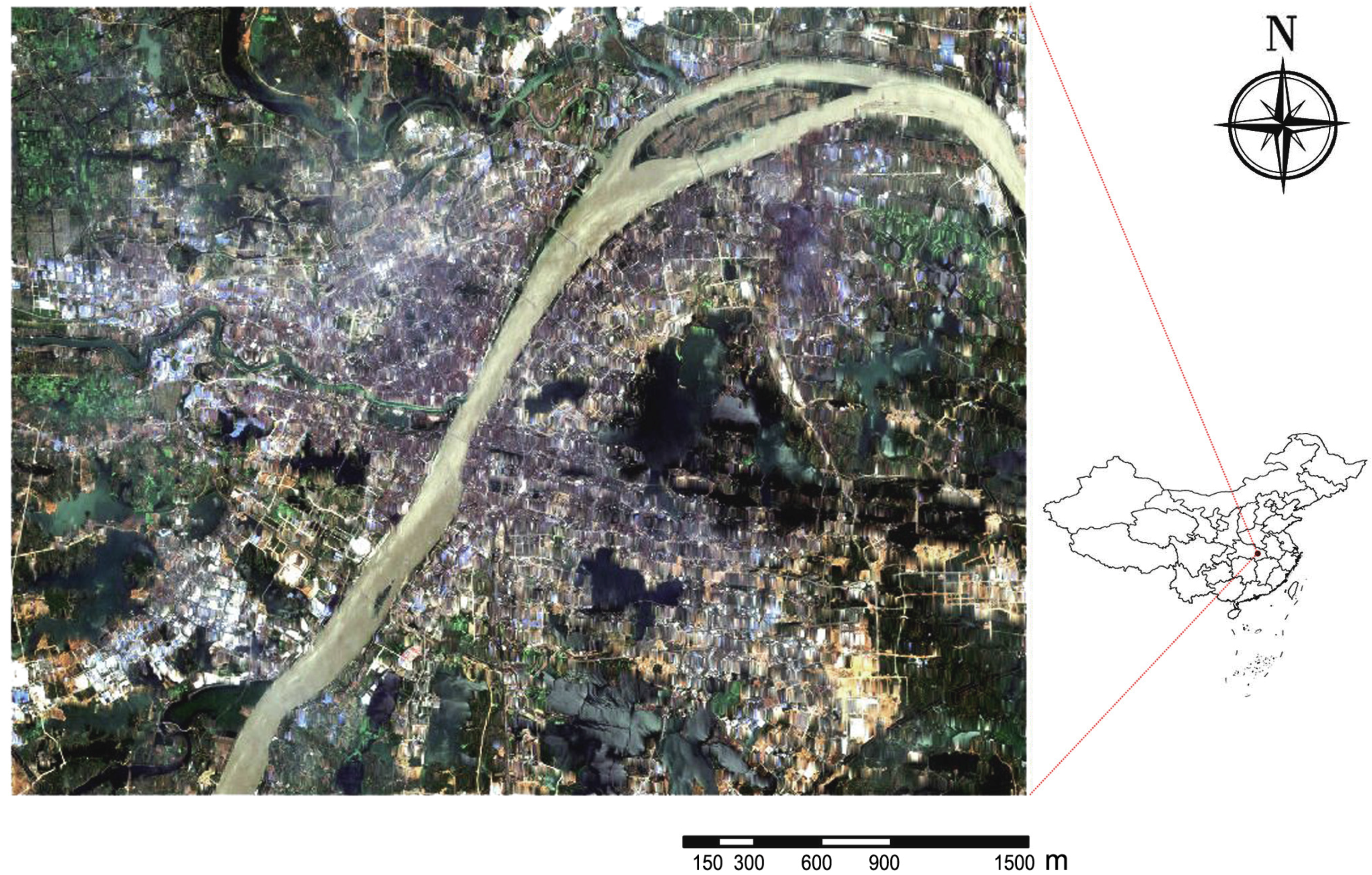
2.1. The Study Area

2.2. The Land Surface Temperature

| Month | MODIS 8-Day LST Data Dates (Julian Dates) | Consecutive Dates with Stable Weather during 8 Days | Average Cloud Cover | Average Wind Velocity | Adapted Pasquill-Gifford Stability Class |
|---|---|---|---|---|---|
| January | 25 (025) | 25–27 | 1.92/8 | 1.33 m/s | G |
| February | 18 (049) | 18–20 | 3.83/8 | 2.25 m/s | F |
| March | 21 (081) | 24–27 | 1.81/8 | 1.38 m/s | G |
| April | 22 (113) | 22–28 | 3.56/8 | 2.13 m/s | F |
| May | 16 (137) | 16–18 | 4.67/8 | 1.38 m/s | G |
| June | 17 (169) | 22–24 | 3.40/8 | 1.25 m/s | G |
| July | 27 (209) | 27–30 | 3.75/8 | 1.38 m/s | G |
| August | 04 (217) | 04–06 | 3.50/8 | 3.48 m/s | F |
| September | 13 (257) | 14–16 | 2.30/8 | 2.21 m/s | F |
| October | 15 (289) | 17–19 | 3.90/8 | 1.45 m/s | G |
| November | 16 (321) | 17–20 | 2.25/8 | 1.45 m/s | G |
| December | 18 (353) | 22–25 | 0.80/8 | 1.80 m/s | G |
| Notation | Adapted Pasquill-Gifford Class | <2 m/s | 2–3 m/s | 3–5 m/s | >5 m/s |
| ≥4/8 Oktas | G | E | D | D | |
| <4/8 Oktas | G | F | E | D |
2.3. The Latent Pattern of the Land Surface Temperature
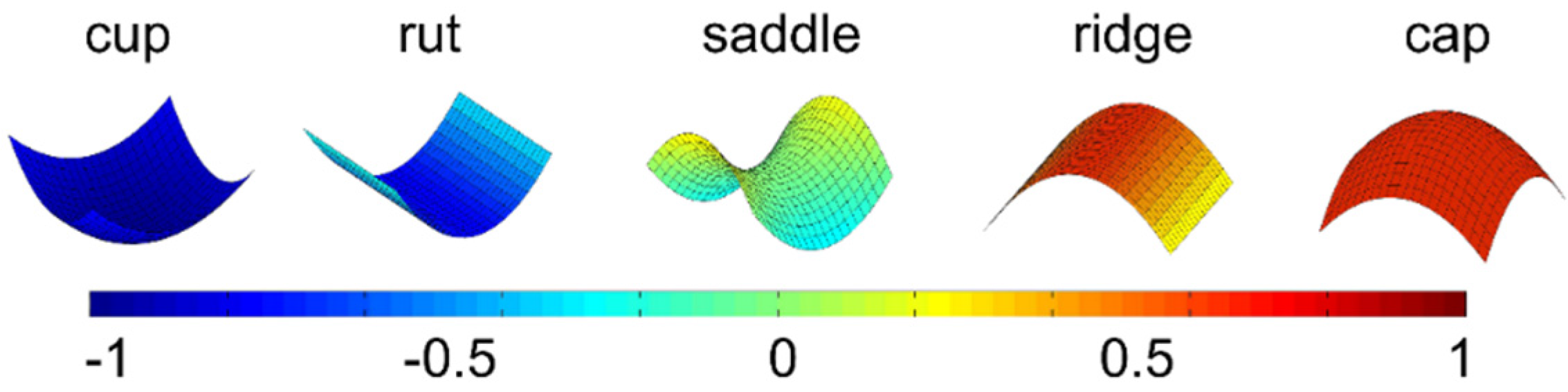
2.4. The Morphology of the Land Surface Temperature

3. Results
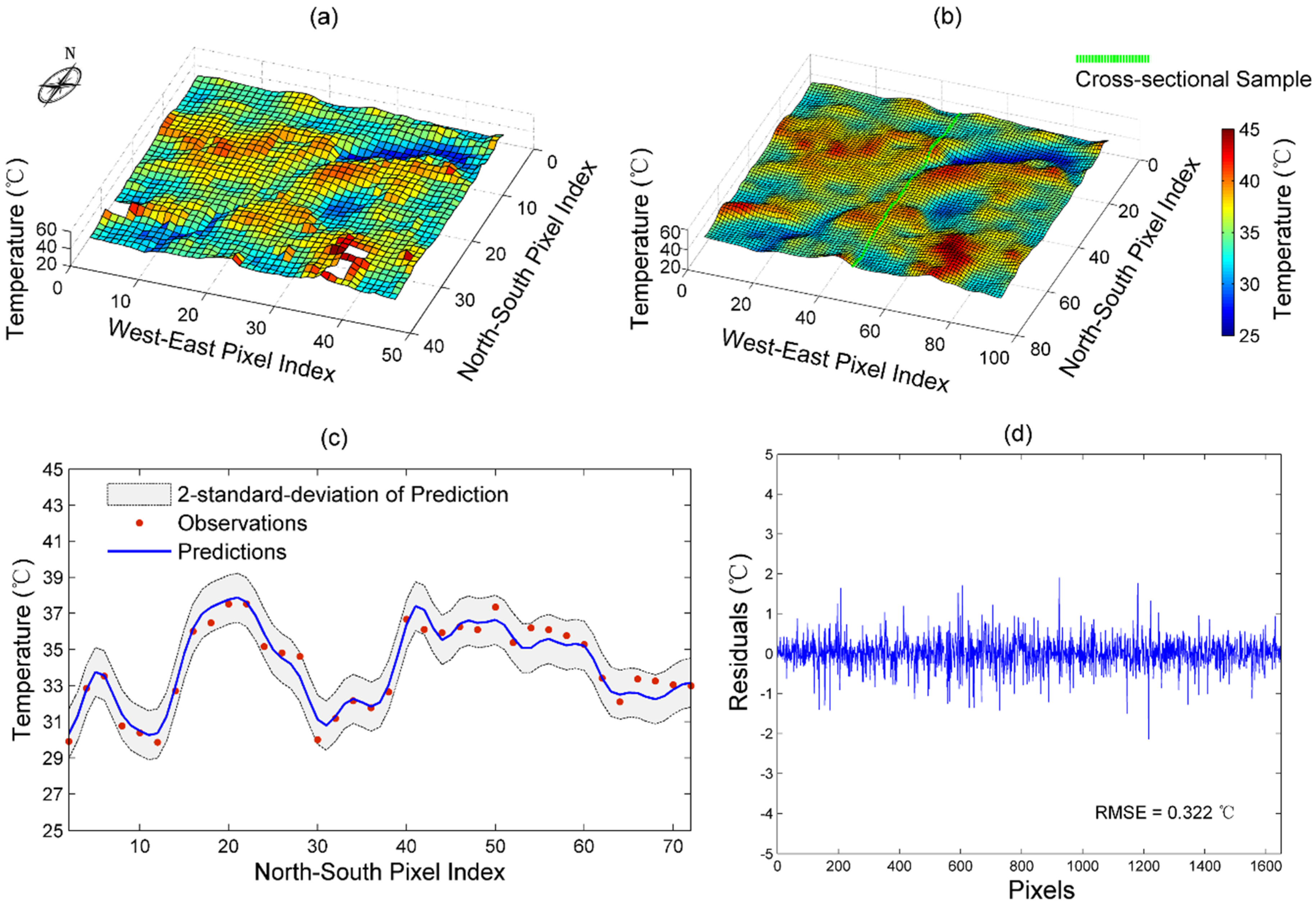
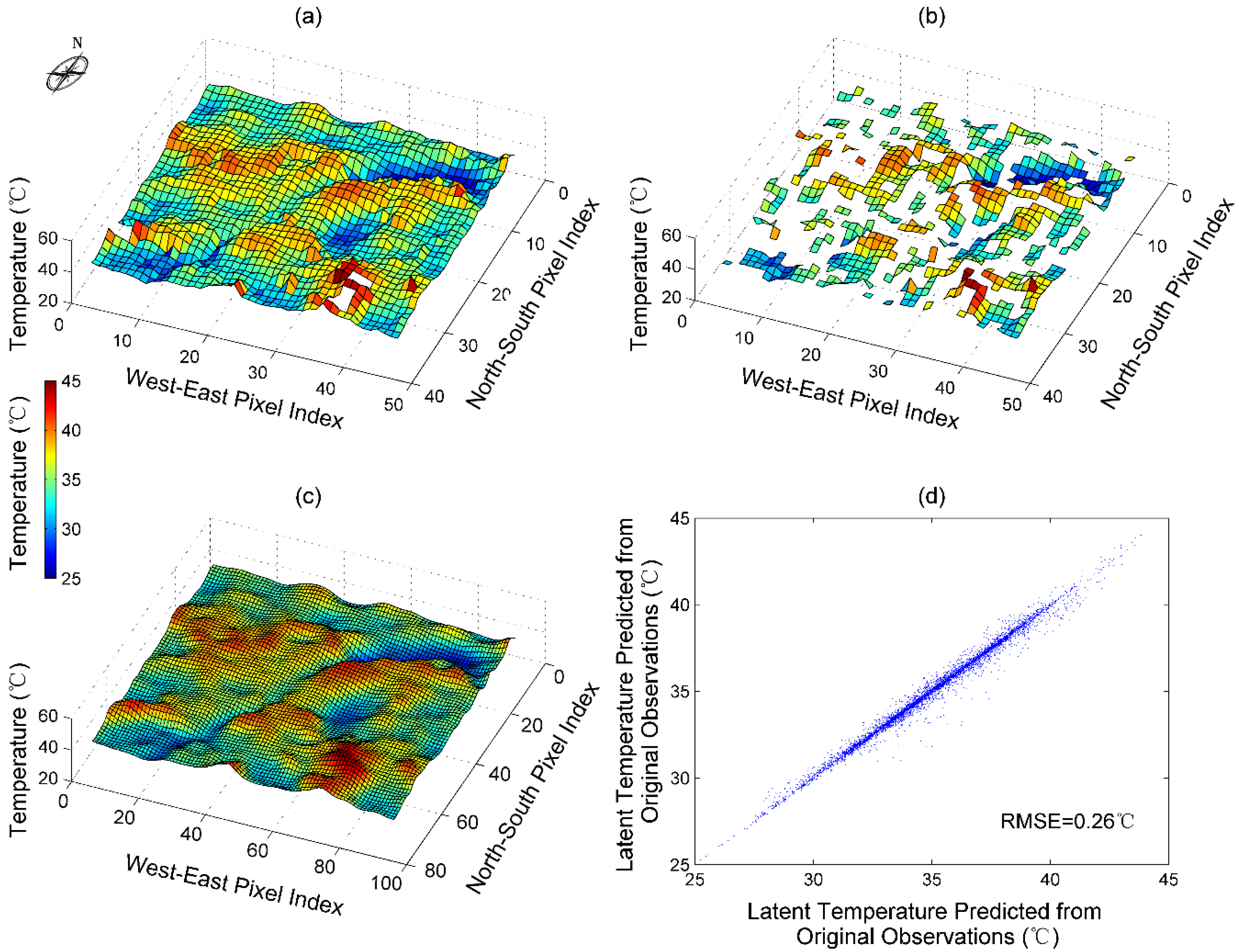
3.1. Latent Pattern of the Land Surface Temperature

| Time | 01:30 | 10:30 | 13:30 | 22:30 | |||||
|---|---|---|---|---|---|---|---|---|---|
| Month | Calendar Date (Julian Date) | RMSE (°C) | Standard Deviation (°C) | RMSE (°C) | Standard Deviation (°C) | RMSE (°C) | Standard Deviation (°C) | RMSE (°C) | Standard Deviation (°C) |
| January | 25(025) | 0.24 | 0.31 | 0.26 | 0.34 | 0.38 | 0.48 | 0.30 | 0.38 |
| February | 18(049) | 0.49 | 0.91 | 0.30 | 0.41 | 0.64 | 0.40 | 0.64 | 0.62 |
| March | 21(081) | 0.20 | 0.46 | 0.26 | 0.57 | 0.36 | 0.36 | 0.36 | 0.26 |
| April | 22(113) | 0.30 | 0.55 | 0.46 | 0.37 | 0.44 | 0.55 | 0.44 | 0.39 |
| May | 16(137) | 0.30 | 0.48 | 0.69 | 0.52 | 0.64 | 0.48 | 0.37 | 0.42 |
| June | 17(169) | 0.34 | 0.34 | 0.78 | 0.43 | 0.64 | 0.34 | 0.27 | 0.46 |
| July | 27(209) | 0.24 | 0.18 | 0.41 | 0.28 | 0.32 | 0.18 | 0.14 | 0.30 |
| August | 04(217) | 0.25 | 0.27 | 0.35 | 0.41 | 0.21 | 0.27 | 0.21 | 0.33 |
| September | 13(257) | 0.30 | 0.44 | 0.44 | 0.50 | 0.33 | 0.46 | 0.33 | 0.42 |
| October | 15(289) | 0.32 | 0.27 | 0.22 | 0.26 | 0.19 | 0.43 | 0.19 | 0.43 |
| November | 16(321) | 0.25 | 0.20 | 0.16 | 0.37 | 0.13 | 0.37 | 0.13 | 0.34 |
| December | 18(353) | 0.23 | 0.37 | 0.49 | 0.32 | 0.26 | 0.32 | 0.28 | 0.31 |

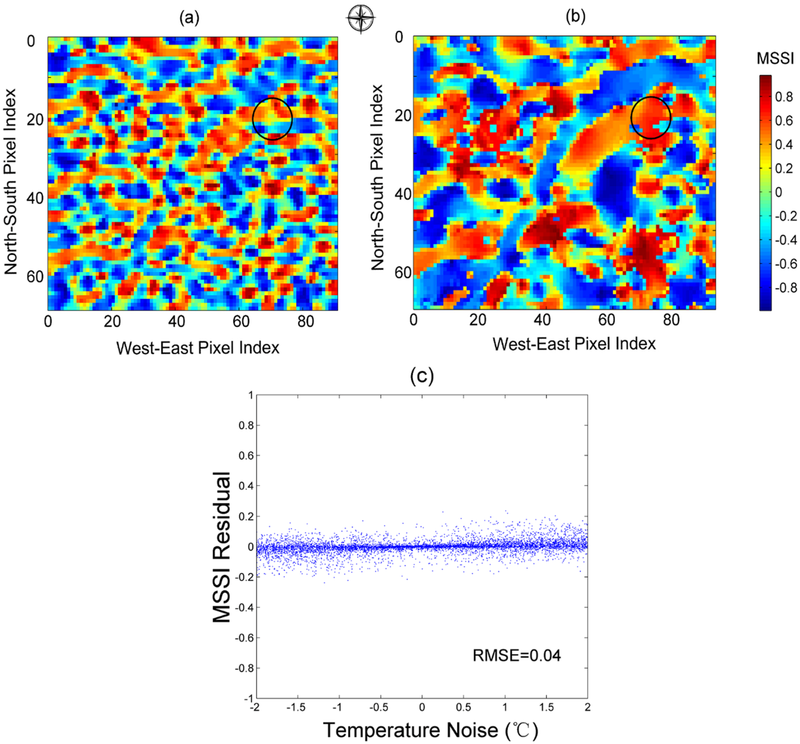
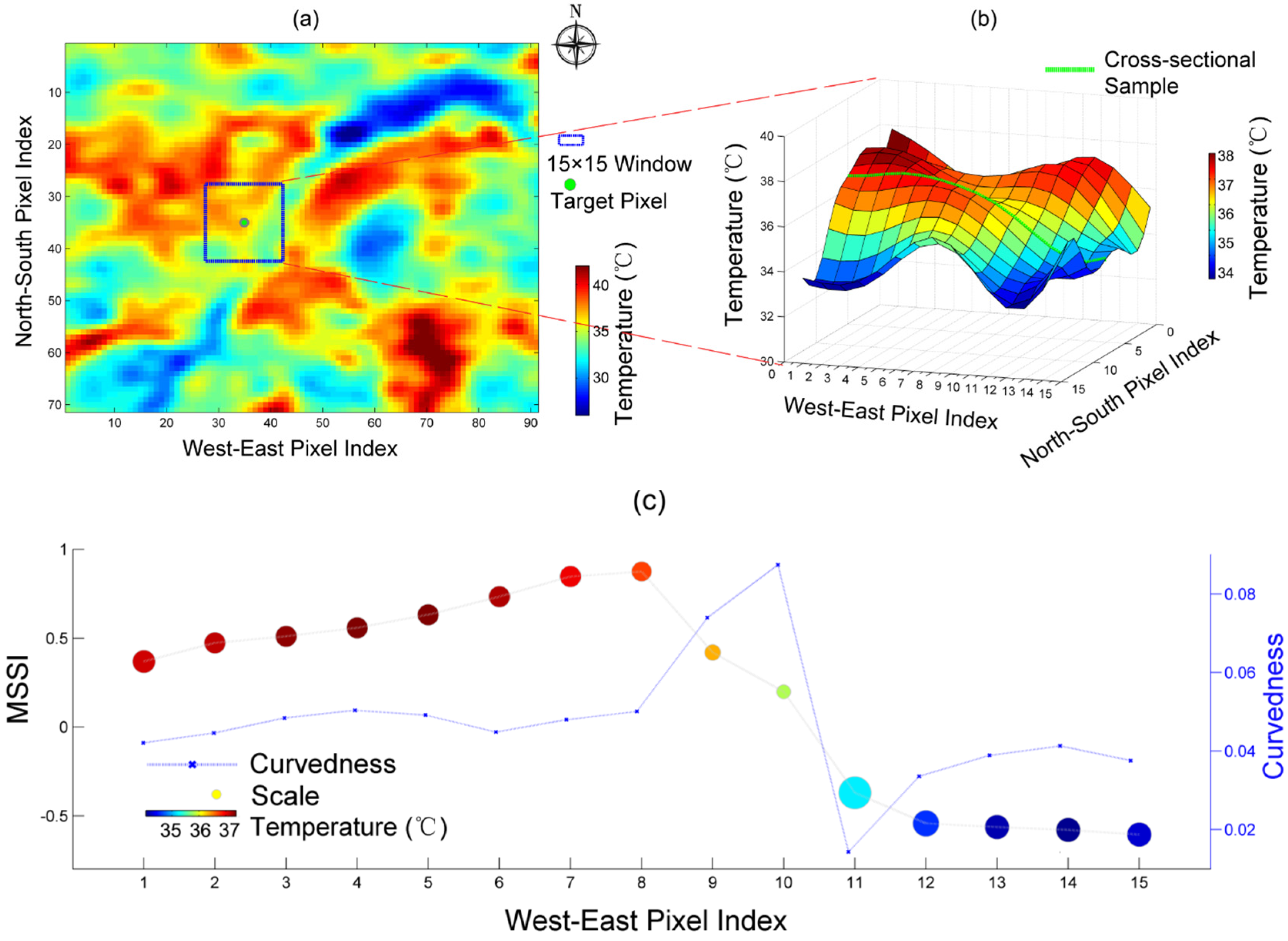
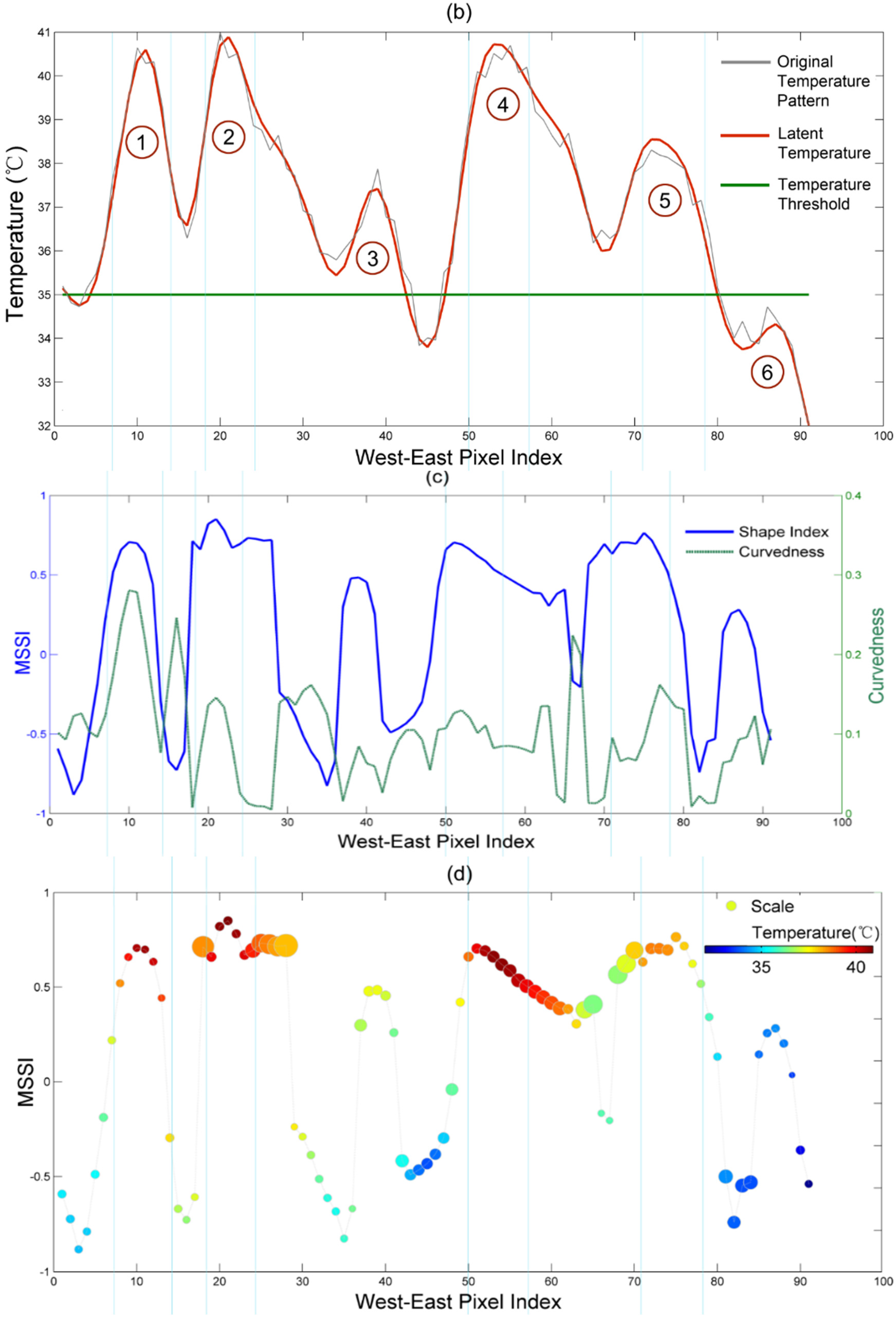
3.2. The Morphology of the Latent LST


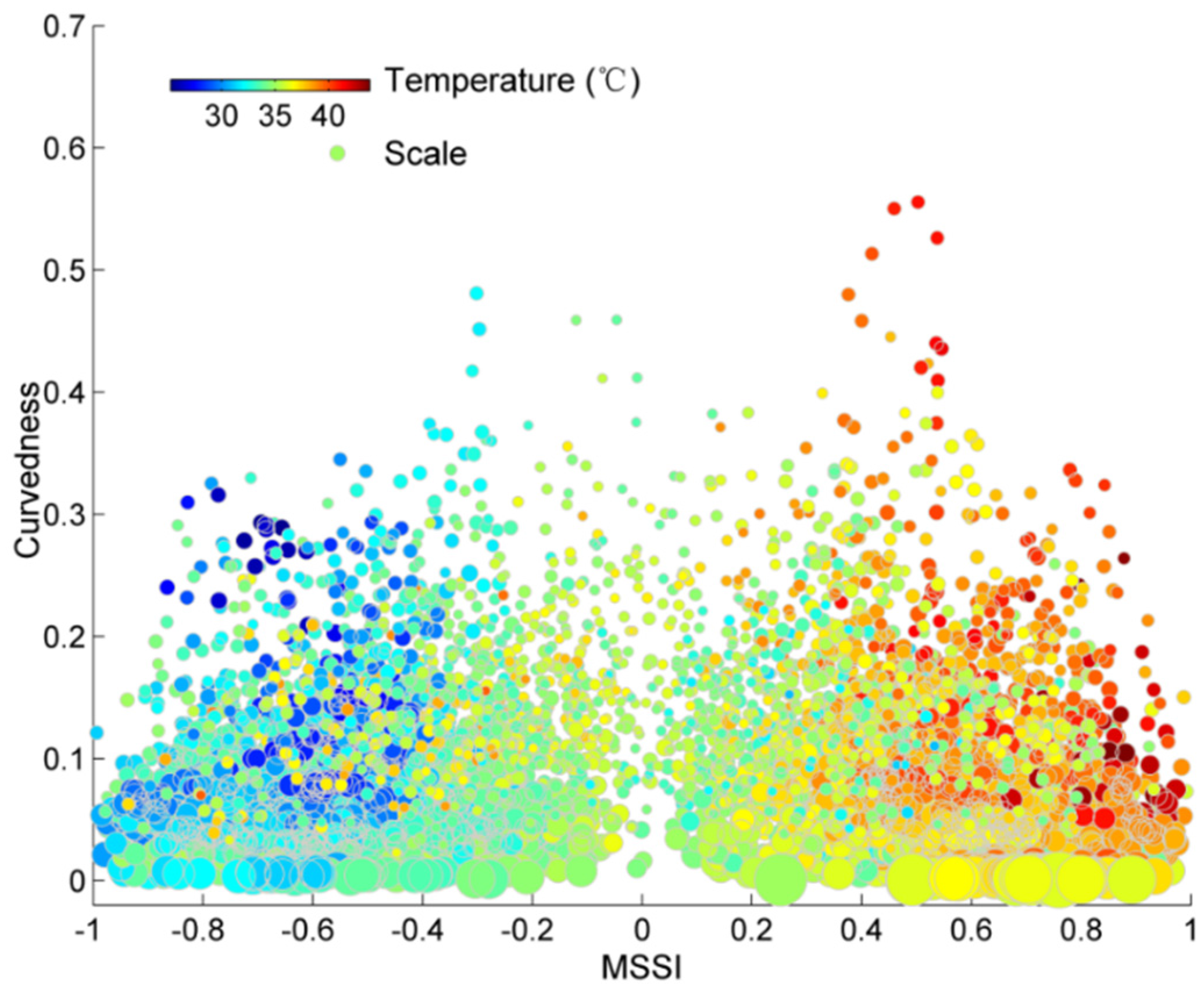
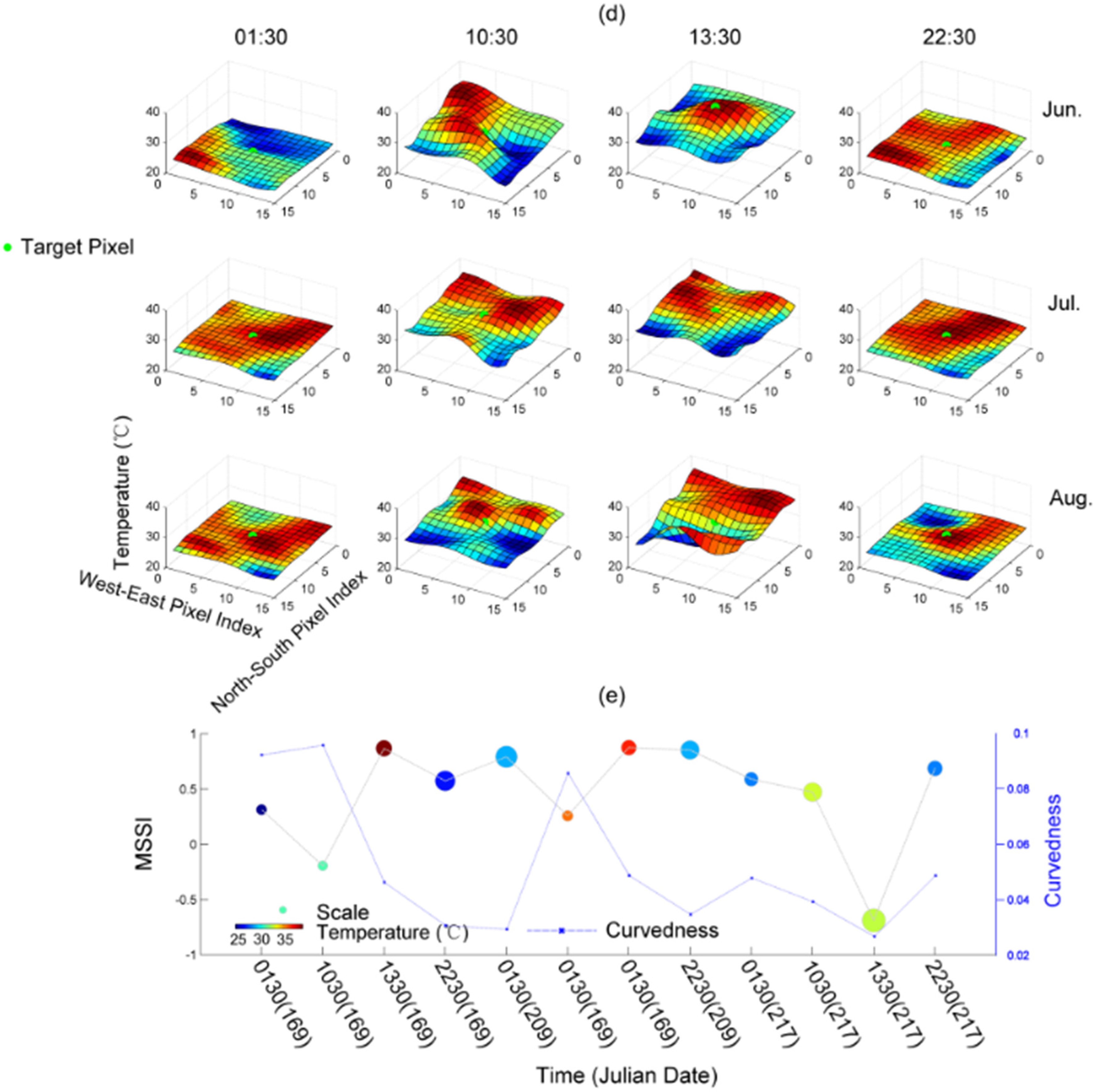
3.3. The Spatial and Temporal Dynamics of the LST Morphology


| Dynamics | Pixel Index | MSSI | Relative Scale (Pixels) | Temperature (°C) | Curvedness |
|---|---|---|---|---|---|
| Sample Spatial Dynamics (13:30 on 27 July) | 1 | 0.37 | 5.22 | 37.10 | 0.04 |
| 2 | 0.47 | 4.55 | 37.16 | 0.05 | |
| 3 | 0.51 | 4.55 | 37.29 | 0.05 | |
| 4 | 0.56 | 4.55 | 37.37 | 0.05 | |
| 5 | 0.63 | 4.55 | 37.34 | 0.05 | |
| 6 | 0.73 | 4.55 | 37.21 | 0.04 | |
| 7 | 0.85 | 4.55 | 37.01 | 0.05 | |
| 8 | 0.88 | 3.96 | 6.73 | 0.05 | |
| 9 | 0.42 | 2.61 | 36.35 | 0.07 | |
| 10 | 0.20 | 1.98 | 35.82 | 0.09 | |
| 11 | −0.37 | 10.45 | 35.19 | 0.01 | |
| 12 | −0.54 | 6.89 | 34.58 | 0.03 | |
| 13 | −0.56 | 6.00 | 34.15 | 0.04 | |
| 14 | −0.58 | 6.00 | 34.03 | 0.04 | |
| 15 | −0.61 | 6.00 | 34.26 | 0.04 | |
| Sample Temporal Dynamics | 1 | 0.31 | 1.98 | 24.25 | 0.09 |
| 2 | −0.19 | 1.72 | 30.79 | 0.09 | |
| 3 | 0.87 | 4.55 | 39.18 | 0.05 | |
| 4 | 0.57 | 6.89 | 26.24 | 0.03 | |
| 5 | 0.79 | 7.92 | 28.52 | 0.03 | |
| 6 | 0.26 | 1.98 | 35.65 | 0.08 | |
| 7 | 0.88 | 3.96 | 36.73 | 0.05 | |
| 8 | 0.85 | 6.00 | 28.58 | 0.03 | |
| 9 | 0.59 | 3.45 | 27.76 | 0.05 | |
| 10 | 0.47 | 6.00 | 32.68 | 0.04 | |
| 11 | −0.69 | 9.09 | 32.61 | 0.03 | |
| 12 | 0.69 | 3.96 | 27.96 | 0.05 |
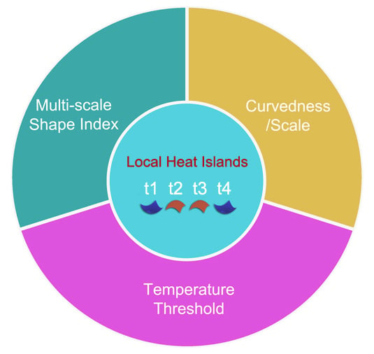
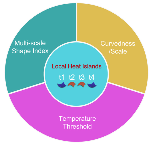
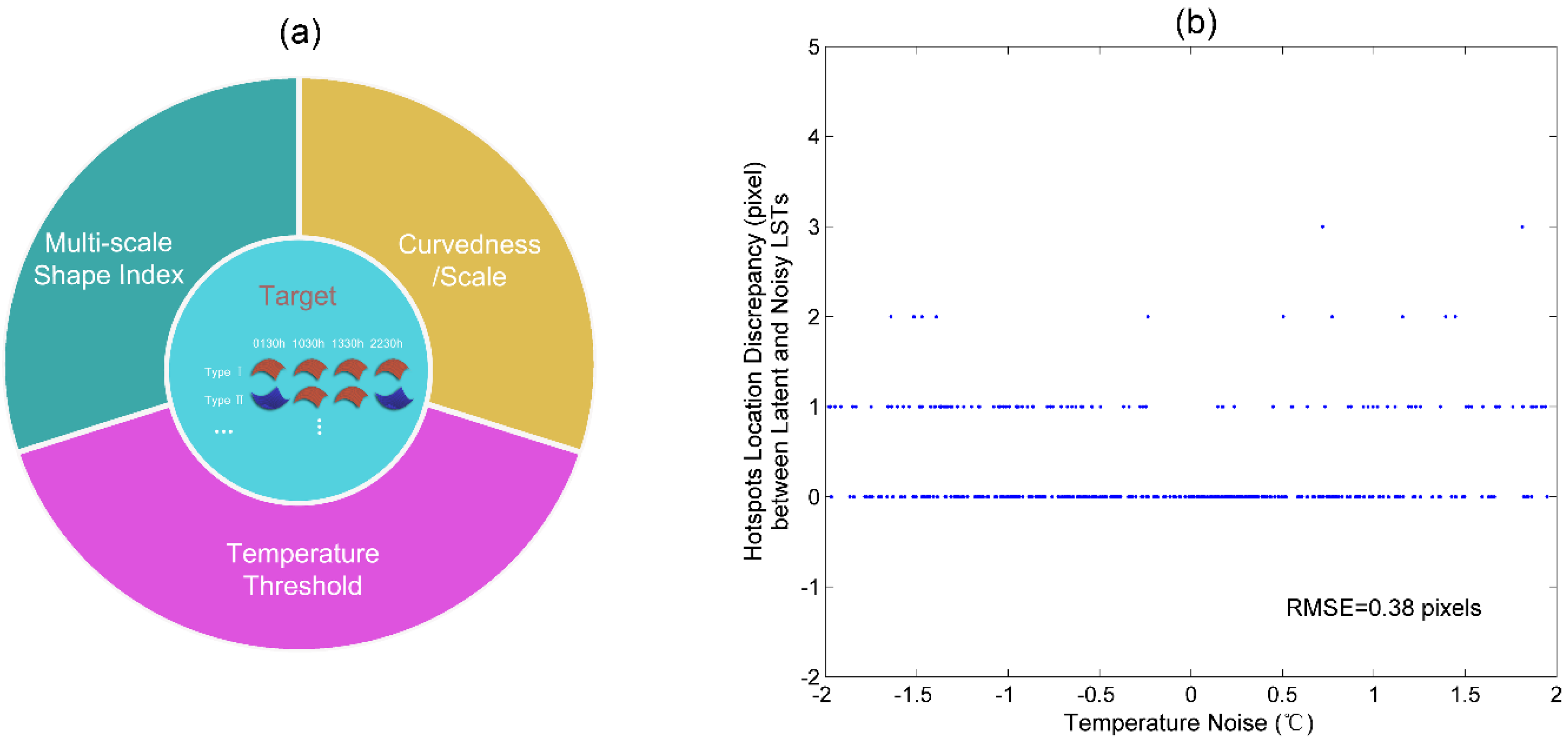
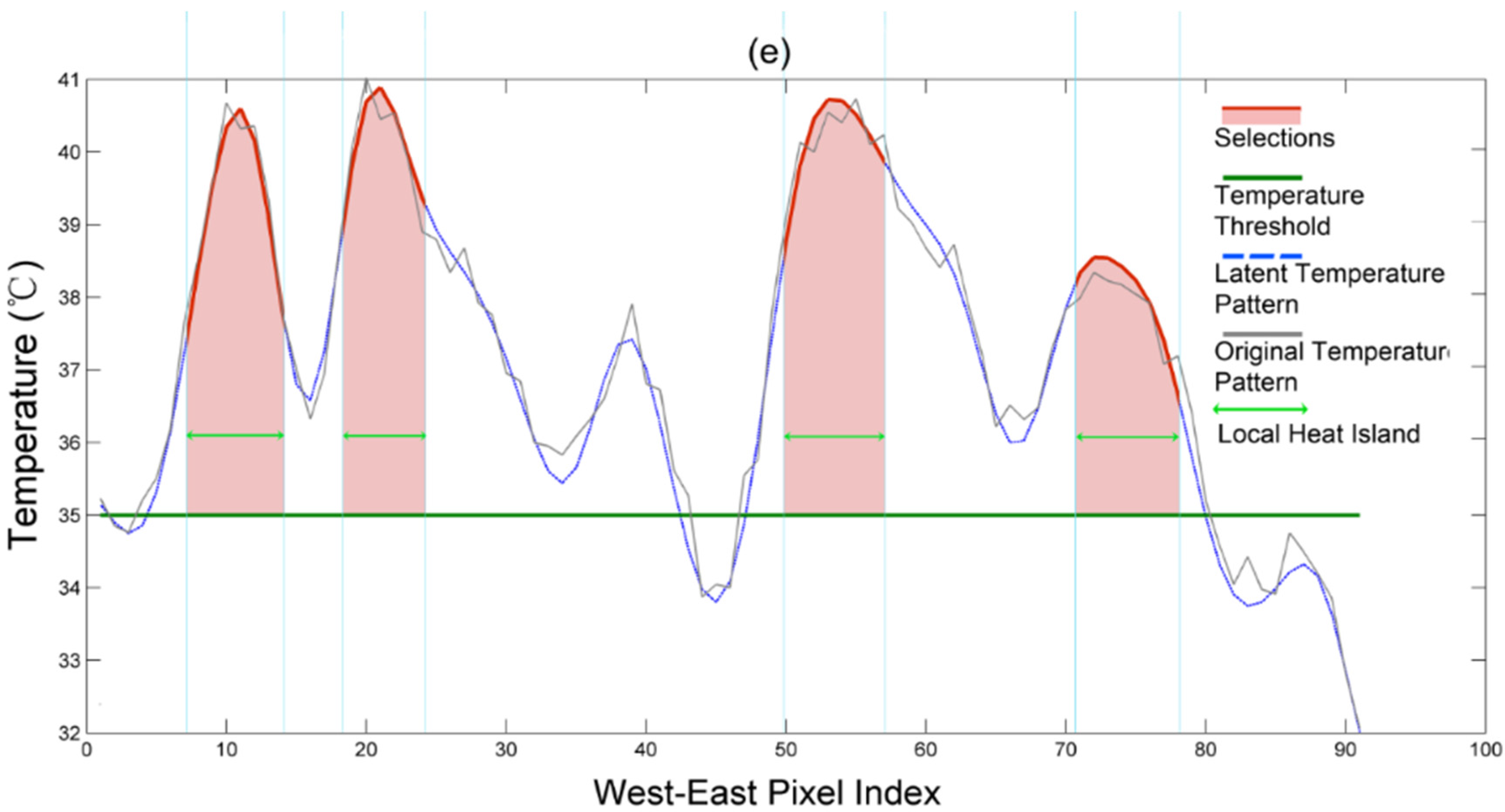
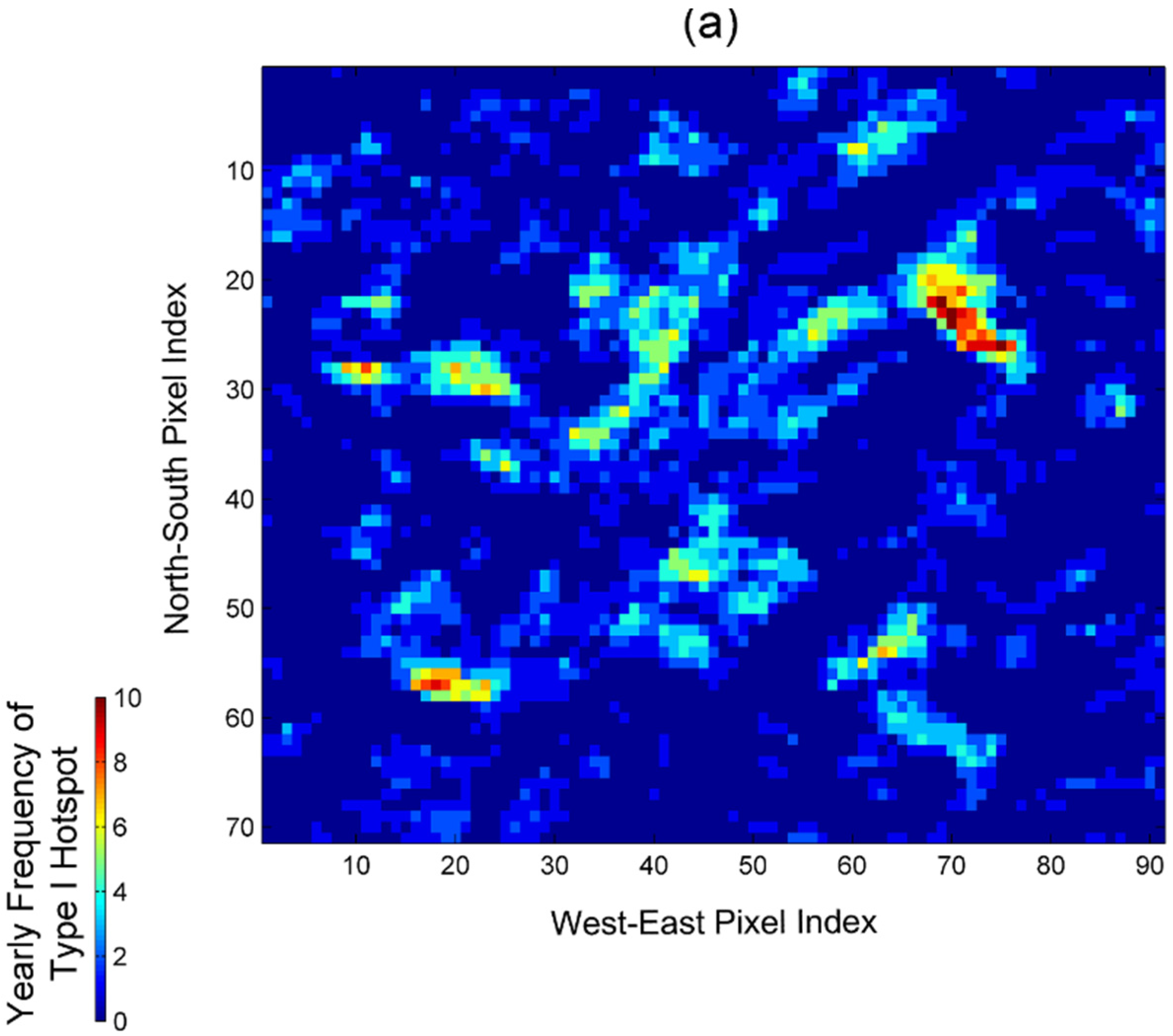
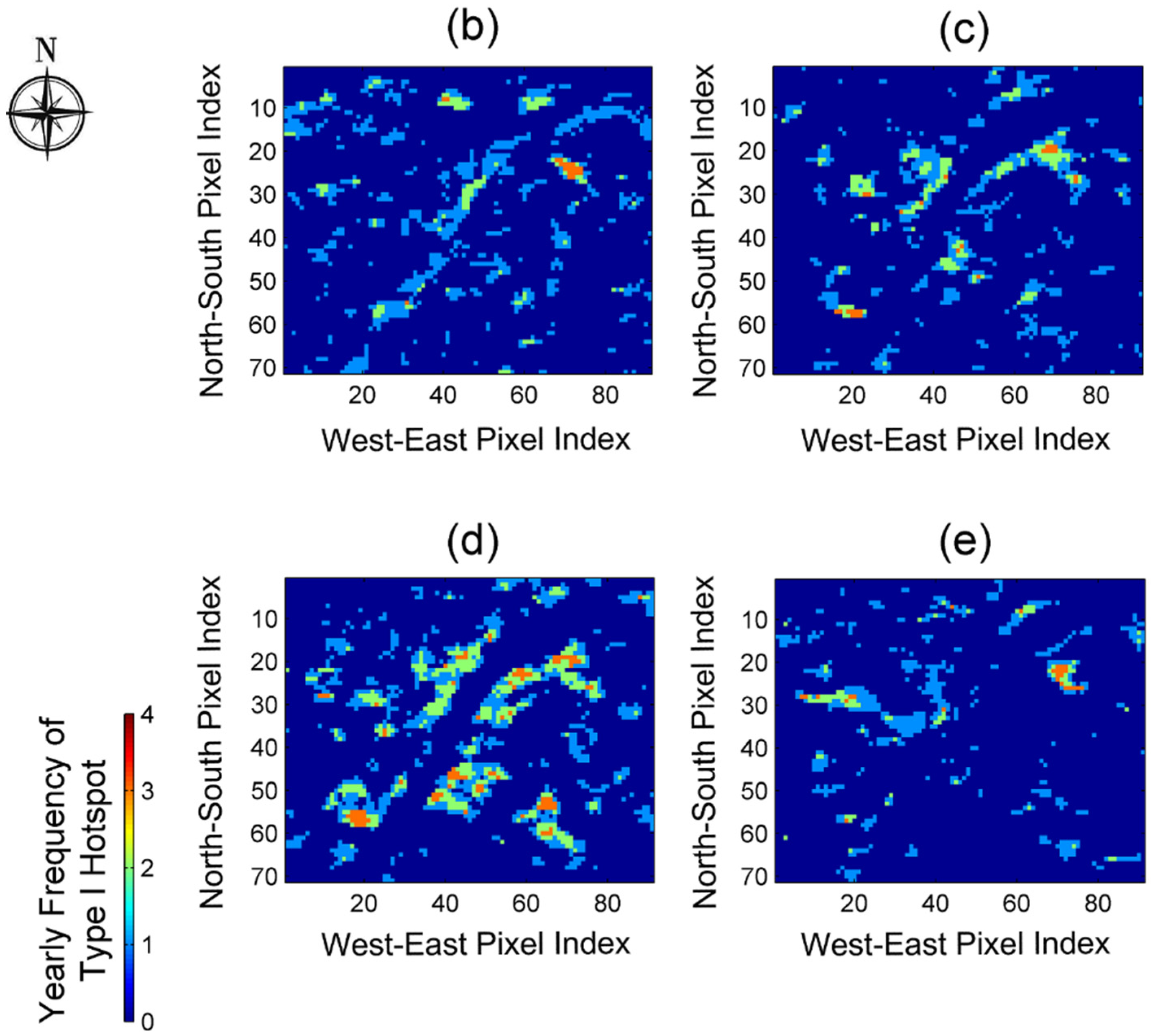
3.4. Identification of the Potential Hotspots


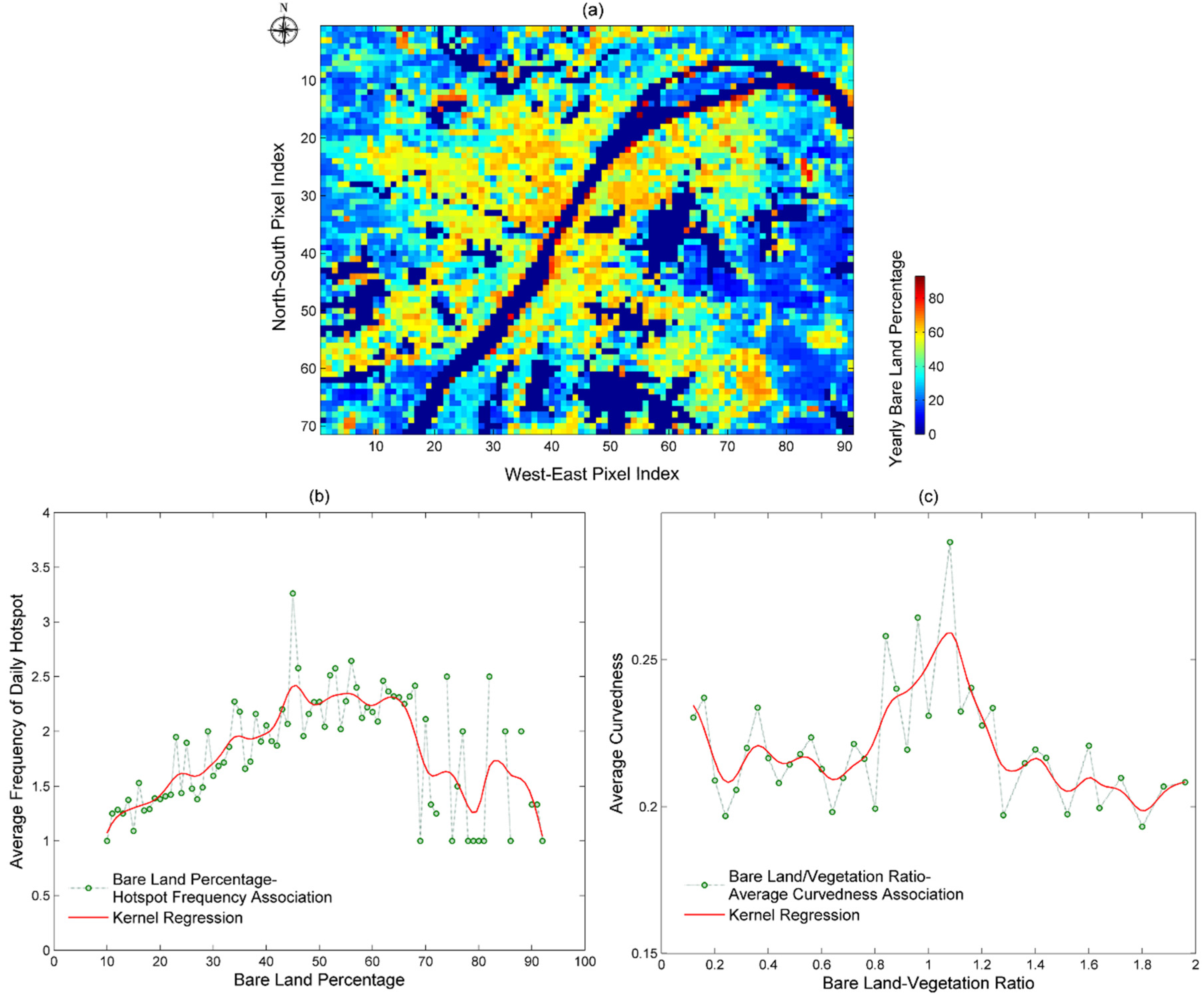
3.5. The Yearly Dynamics of the Hotspots-Land Surface Composition Relationship
| Gaussian Distribution Parameters | μ | σ | 2 × σ | 2 × σ Greater than 0 |
|---|---|---|---|---|
| 3-Gaussian-Distribution Mixture | 0.02 | 0.10 | 0.20 | 0.22 |
| 0.51 | 0.04 | 0.08 | \ | |
| −0.52 | 0.05 | 0.09 | \ |


4. Discussion
4.1. The Scale of Investigation
4.2. Phenomena Study and the Planning Profession
4.3. The Indicators for Characterizing LST Patterns
4.4. Understanding the Urban Environmental Process
4.5. Hypothesis, Model Feasibility and Data
5. Conclusions
Acknowledgments
Author Contributions
Conflicts of Interest
References
- Stone, B. Urban and rural temperature trends in proximity to large us cities: 1951–2000. Int. J. Clim. 2007, 27, 1801–1807. [Google Scholar] [CrossRef]
- Manley, G. On the frequency of snowfall in metropolitan england. Q. J. R. Meteorol. Soc. 1958, 84, 70–72. [Google Scholar] [CrossRef]
- Landsberg, H.E. The Urban Climate; Academic Press: New York, NY, USA, 1981; Volume 28. [Google Scholar]
- Oke, T.R. Canyon geometry and the nocturnal urban heat island: Comparison of scale model and field observations. J. Clim. 1981, 1, 237–254. [Google Scholar] [CrossRef]
- Oke, T.R. The energetic basis of the urban heat island. Q. J. R. Meteorol. Soc. 1982, 108, 1–24. [Google Scholar] [CrossRef]
- Howard, L. The Climate of London: Deduced from Meteorological Observations Made in the Metropolis and at Various Places Around It; Harvey and Darton: London, UK, 1833; Volume 2. [Google Scholar]
- Oke, T.R. The distinction between canopy and boundary-layer urban heat islands. Atmosphere 1976, 14, 268–277. [Google Scholar]
- Kalnay, E.; Cai, M. Impact of urbanization and land-use change on climate. Nature 2003, 423, 528–531. [Google Scholar] [CrossRef] [PubMed]
- Stone, B.; Vargo, J.; Habeeb, D. Managing climate change in cities: Will climate action plans work? Landsc. Urban. Plan. 2012, 107, 263–271. [Google Scholar] [CrossRef]
- Voogt, J.A.; Oke, T.R. Thermal remote sensing of urban climates. Remote Sens. Environ. 2003, 86, 370–384. [Google Scholar] [CrossRef]
- Li, Z.-L.; Tang, B.-H.; Wu, H.; Ren, H.; Yan, G.; Wan, Z.; Trigo, I.F.; Sobrino, J.A. Satellite-derived land surface temperature: Current status and perspectives. Remote Sens. Environ. 2013, 131, 14–37. [Google Scholar] [CrossRef]
- Anderson, M.; Norman, J.; Kustas, W.; Houborg, R.; Starks, P.; Agam, N. A thermal-based remote sensing technique for routine mapping of land-surface carbon, water and energy fluxes from field to regional scales. Remote Sens. Environ. 2008, 112, 4227–4241. [Google Scholar] [CrossRef]
- De Kauwe, M.G.; Taylor, C.M.; Harris, P.P.; Weedon, G.P.; Ellis, R.J. Quantifying land surface temperature variability for two sahelian mesoscale regions during the wet season. J. Hydrometeorol. 2013, 14, 1605–1619. [Google Scholar] [CrossRef]
- Sobrino, J.; Oltra-Carrió, R.; Sòria, G.; Bianchi, R.; Paganini, M. Impact of spatial resolution and satellite overpass time on evaluation of the surface urban heat island effects. Remote Sens. Environ. 2012, 117, 50–56. [Google Scholar] [CrossRef]
- Roth, M.; Oke, T.; Emery, W. Satellite-derived urban heat islands from three coastal cities and the utilization of such data in urban climatology. Int. J. Remote Sens. 1989, 10, 1699–1720. [Google Scholar] [CrossRef]
- Voogt, J.A.; Oke, T.R. Complete urban surface temperatures. J. Appl. Meteorol. 1997, 36, 1117–1132. [Google Scholar] [CrossRef]
- Weng, Q. Thermal infrared remote sensing for urban climate and environmental studies: Methods, applications, and trends. ISPRS J. Photogramm. Remote Sens. 2009, 64, 335–344. [Google Scholar] [CrossRef]
- Schwarz, N.; Schlink, U.; Franck, U.; Großmann, K. Relationship of land surface and air temperatures and its implications for quantifying urban heat island indicators—An application for the city of leipzig (germany). Ecol. Indic. 2012, 18, 693–704. [Google Scholar] [CrossRef]
- Streutker, D.R. A remote sensing study of the urban heat island of houston, Texas. Int. J. Remote Sens. 2002, 23, 2595–2608. [Google Scholar] [CrossRef]
- Streutker, D.R. Satellite-measured growth of the urban heat island of houston, Texas. Remote Sens. Environ. 2003, 85, 282–289. [Google Scholar] [CrossRef]
- Rajasekar, U.; Weng, Q. Urban heat island monitoring and analysis using a non-parametric model: A case study of Indianapolis. ISPRS J. Photogramm. Remote Sens. 2009, 64, 86–96. [Google Scholar] [CrossRef]
- Wheeler, S.M. State and municipal climate change plans: The first generation. J. Am. Plan. Assoc. 2008, 74, 481–496. [Google Scholar] [CrossRef]
- Betsill, M.; Rabe, B. Climate change and multilevel governance: The evolving state and local roles. In Toward Sustainable Communities: Transition and Transformations in Environmental Policy; MIT Press: Cambridge, MA, USA, 2009. [Google Scholar]
- Griggs, D.J.; Noguer, M. Climate change 2001: The scientific basis. Contribution of working group i to the third assessment report of the intergovernmental panel on climate change. Weather 2002, 57, 267–269. [Google Scholar] [CrossRef]
- Valleron, A.; Boumendil, A. Epidemiology and heat waves: Analysis of the 2003 episode in France. Comptes Rend. Biol. 2004, 327, 1125–1141. [Google Scholar] [CrossRef]
- Prevention. Heat-related mortality—Arizona, 1993–2002, and united states, 1979–2002. Morb. Mortal. Wkly. Report 2005, 54, 628–630. [Google Scholar]
- Kalkstein, L.; Koppe, C.; Orlandini, S.; Sheridan, S.; Smoyer-Tomic, K. Health impacts of heat: Present realties and potential impacts of climate change. In Distributional Impacts of Climate Change and Disasters; Edward Elgar: Cheltenham, UK, 2009; pp. 69–81. [Google Scholar]
- Stewart, I.D. A systematic review and scientific critique of methodology in modern urban heat island literature. Int. J. Clim. 2011, 31, 200–217. [Google Scholar] [CrossRef]
- Chang, C.-R.; Li, M.-H.; Chang, S.-D. A preliminary study on the local cool-island intensity of taipei city parks. Landsc. Urban Plan. 2007, 80, 386–395. [Google Scholar] [CrossRef]
- Eliasson, I. The use of climate knowledge in urban planning. Landsc. Urban Plan. 2000, 48, 31–44. [Google Scholar] [CrossRef]
- Arnfield, J. Two decades of urban climate research: A review of turbulence exchanges of energy and water, and the urban heat island. Inter. J. Clim. 2003, 23, 1–26. [Google Scholar] [CrossRef]
- Quan, J.; Chen, Y.; Zhan, W.; Wang, J.; Voogt, J.; Wang, M. Multi-temporal trajectory of the urban heat island centroid in Beijing, China based on a gaussian volume model. Remote Sens. Environ. 2014, 149, 33–46. [Google Scholar] [CrossRef]
- Wan, Z.; Dozier, J. A generalized split-window algorithm for retrieving land-surface temperature from space. IEEE Trans. Geosci. Remote Sens. 1996, 34, 892–905. [Google Scholar]
- Wan, Z.; Zhang, Y.; Zhang, Q.; Li, Z.-L. Quality assessment and validation of the modis global land surface temperature. Inter. J. Remote Sens. 2004, 25, 261–274. [Google Scholar] [CrossRef]
- Wan, Z. New refinements and validation of the MODIS land-surface temperature/emissivity products. Remote Sens. Environ. 2008, 112, 59–74. [Google Scholar] [CrossRef]
- Wan, Z. New refinements and validation of the collection-6 modis land-surface temperature/emissivity product. Remote Sens. Environ. 2014, 140, 36–45. [Google Scholar] [CrossRef]
- Pasquill, F.; Smith, F. Atmospheric Diffusion: Study of the Dispersion of Windborne Material from Industrial and other Sources; John Wiley & Sons: New York, NY, USA, 1983. [Google Scholar]
- Tomlinson, C.; Chapman, L.; Thornes, J.; Baker, C. Derivation of Birmingham's summer surface urban heat island from MODIS satellite images. Int. J. Clim. 2012, 32, 214–224. [Google Scholar] [CrossRef]
- Chapman, L.; Thornes, J.E.; Bradley, A.V. Modelling of road surface temperature from a geographical parameter database. Part 1: Statistical. Meteorol. Appl. 2001, 8, 409–419. [Google Scholar] [CrossRef]
- Goodchild, M.F. A spatial analytical perspective on geographical information systems. Int. J. Geogr. Inf. Syst. 1987, 1, 327–334. [Google Scholar] [CrossRef]
- Goodchild, M.F. Integrating GIS and remote sensing for vegetation analysis and modeling: Methodological issues. J. Veg. Sci. 1994, 5, 615–626. [Google Scholar] [CrossRef]
- Bonilla, E.V.; Chai, K.M.; Williams, C. Multi-task gaussian process prediction. In Advances in Neural Information Processing Systems; Donnelley & Sons: San Francisco, CA, USA, 2008. [Google Scholar]
- Rasmussen, C.E. Gaussian Processes for Machine Learning. In Advanced Lectures on Machine Learning; Springer: Heidelberg, Germany, 2004; pp. 63–71. [Google Scholar]
- Blumer, A.; Ehrenfeucht, A.; Haussler, D.; Warmuth, M.K. Occam's razor. Inf. Proc. Lett. 1987, 24, 377–380. [Google Scholar] [CrossRef]
- Bonde, U.; Badrinarayanan, V.; Cipolla, R. Multi Scale Shape Index for 3D Object Recognition; Springer: Heidelberg, Germany, 2013. [Google Scholar]
- Koenderink, J.J.; van Doorn, A.J. Surface shape and curvature scales. Imag. Vis. Comput. 1992, 10, 557–564. [Google Scholar] [CrossRef]
- Lindeberg, T. Feature detection with automatic scale selection. Int. J. Comput. Vis. 1998, 30, 79–116. [Google Scholar] [CrossRef]
- Lowe, D.G. Object recognition from local scale-invariant features, computer vision. Proc. IEEE 1999, 2, 1150–1157. [Google Scholar]
- DiMiceli, C.; Carroll, M.; Sohlberg, R.; Huang, C.; Hansen, M.; Townshend, J. Annual Global Automated Modis Vegetation Continuous Fields (Mod44b) at 250 m Spatial Resolution for Data Years beginning Day 65, 2000–2010, Collection 5 percent Tree Cover; University of Maryland: Maryland, MD, USA, 2011. [Google Scholar]
- Sayre, N.F. Ecological and geographical scale: Parallels and potential for integration. Prog. Hum. Geogr. 2005, 29, 276–290. [Google Scholar] [CrossRef]
- Sayre, N.F. Scale. Wiley Online Libr. 2009. [Google Scholar] [CrossRef]
- Rizwan, A.M.; Dennis, L.Y.; Liu, C. A review on the generation, determination and mitigation of urban heat island. J. Environ. Sci. 2008, 20, 120–128. [Google Scholar] [CrossRef]
- Zhou, D.C.; Zhao, S.Q.; Liu, S.G.; Zhang, L.X.; Zhu, C. Surface urban heat island in China’s 32 major cities: Spatial patterns and drivers. Remote Sens. Environ. 2014, 152, 51–61. [Google Scholar] [CrossRef]
- Podobnikar, T.; Ostir, K.; Zaksek, K. Influence of data quality on solar radiation modeling. In Gis for Sustainable Development; Campagna, M., Ed.; CRC Press, Taylor & Francis Group: Boca Raton, FL, USA, 2006; pp. 417–430. [Google Scholar]
© 2015 by the authors; licensee MDPI, Basel, Switzerland. This article is an open access article distributed under the terms and conditions of the Creative Commons by Attribution (CC-BY) license (http://creativecommons.org/licenses/by/4.0/).
Share and Cite
Wang, J.; Zhan, Q.; Guo, H. The Morphology, Dynamics and Potential Hotspots of Land Surface Temperature at a Local Scale in Urban Areas. Remote Sens. 2016, 8, 18. https://0-doi-org.brum.beds.ac.uk/10.3390/rs8010018
Wang J, Zhan Q, Guo H. The Morphology, Dynamics and Potential Hotspots of Land Surface Temperature at a Local Scale in Urban Areas. Remote Sensing. 2016; 8(1):18. https://0-doi-org.brum.beds.ac.uk/10.3390/rs8010018
Chicago/Turabian StyleWang, Jiong, Qingming Zhan, and Huagui Guo. 2016. "The Morphology, Dynamics and Potential Hotspots of Land Surface Temperature at a Local Scale in Urban Areas" Remote Sensing 8, no. 1: 18. https://0-doi-org.brum.beds.ac.uk/10.3390/rs8010018