1. Introduction
Airborne light detection and ranging (LiDAR) technology has been developing very rapidly in recent years. Since it can obtain a high density point cloud of three-dimensional (3D) information, and does not suffer the effect of outside light conditions, this technology has been widely used in various fields, such as digital terrain model (DTM) generation [
1,
2,
3], 3D city model construction [
4,
5], road extraction [
6,
7] and many others. For most applications, point cloud filtering is a crucial step which directly affects the precision of model building or feature extraction.
Over the years, several filtering algorithms have been proposed and applied successfully to airborne LiDAR point cloud. These algorithms can be classified into three categories namely, slope-based filtering algorithms [
8,
9,
10,
11], interpolation-based filtering algorithms [
2,
12,
13,
14,
15,
16] and morphology-based filtering algorithms [
17,
18,
19,
20,
21,
22]. A slope-based filtering algorithm was first proposed by Vosselman [
8]. Its basic principle is that through calculating the slope between two adjacent points, the point whose slope value is greater than the threshold is classified as a non-ground point. Thus, filtering effect directly depends on the slope threshold setting. To improve the filtering effect in the highly varied terrain, Sithole [
9] and Susaki [
11] made the slope threshold to be dynamically tuned according to the actual terrain. The Experiments showed an improved performance in complicated environments.
Kraus and Peifger [
12] proposed an interpolation-based algorithm. This method establishes a reference surface using equal weights to all points, and then calculates the residual of each point from this surface. A point with a negative residual is given a greater weight, while a point with a positive residual is given a lesser weight. This is an iterative process whereby at each iteration, points with a smaller weight are filtered. The iteration ends when residuals of all points have fallen below the given threshold. Axelsson [
13] introduced adaptive triangulated irregular networks (TIN) models for filtering. Firstly, a sparse TIN based on ground seeds was built. Then the iteration angle and iteration distance of each point to the TIN was calculated. Points whose iteration angle and distance were both less than the threshold were added and a new TIN created. The process was iterated until no more points could be added. Lin [
2] improved this method by carrying out a segmentation to the point cloud. Adaptive TIN filter was then applied to the segmentation results. The Experiment shows that compared with the Axelsson’s method, Lin’s method reduced omission errors and total errors by 18.26% and 11.47%. Mongus and Žalik [
14] put forward a multi-level interpolation filtering algorithm which does not require any parameter. At each level, a thin plate spline surface interpolation is used to obtain a reference surface with filtering performed according to the residual of each point which is actually the distance to the reference surface. The filtering window keeps on downsizing in a top-down fashion until the desired DTM resolution is obtained. Chen
et al. [
15] improved this method by exploring a filtering judgment that is not based on one residual, but nine residuals which include eight other residuals with its eight neighbors. If a point has at least four residuals smaller than the threshold, it will be included into the group of ground points. This can greatly reduce the possibility of misjudgment caused by the interpolation fitting error. Maguya
et al. [
16] applied an interpolation-based algorithm to challenging forested terrain, where data density is low. In their method, a series of coarse DTMs are generated iteratively and then combined to form the final DTM. This algorithm suites well for steep terrain with very dense vegetation on top.
A morphology-based filtering algorithm usually needs to conduct morphological opening or closing operations directly or indirectly on the point cloud [
23]. This kind of method is simple in principle and easy to implement [
18], but it is hard to decide the filtering window, which is generally referred to as structuring element. A small structuring element can effectively filter out small objects, but it cannot correct errors associated with larger objects such as buildings; while a larger structuring element can effectively filter out larger objects, but it easily flattens terrain details, such as ridges, cliffs, and mountain peaks [
24]. In view of these challenges, Zhang
et al. [
17] have put forward a progressive morphological filtering method. In this method, the structuring element increases gradually, while the elevation difference threshold changes according to the size of structuring element. By calculating elevation difference between morphological opening operation before and after, points whose elevation difference is greater than the threshold are included into ground points. However, this algorithm presupposes that the slope of the area is a constant which is obviously unreasonable.
Chen
et al. [
18] expanded the algorithm proposed by Zhang
et al. [
17] from 1D to 2D. Their method does not need to assume a constant slope, which enhances its applicability in terrains with fluctuation. However, this algorithm needs to set lots of parameters by trial and error, which is a challenge. To address these problems, Chen
et al. [
19] proposed an edge-based morphological filtering algorithm which reduced the number of parameters from seven to two and simplified the calculation. Li
et al. [
20] introduced a gradient-constrained morphological filtering algorithm. In their method, morphological filtering was applied by first identifying gradient feature points (GFPs) using morphological gradients, which locate the potential object points prior to filtering. In doing so, computation efficiency can be speed up and terrain features can also be preserved. In addition, Li
et al. [
21] proposed a top-hat morphological algorithm with sloped brim capable of suppressing omission errors caused by protruding terrain features. To achieve the same effect, Li
et al. [
22] improved the top-hat filter by executing directional edge constraints along scan lines whose directions are from left to right on every row of the index grid and from bottom to top on every column of the index grid. Judging the two end points of each point sequence makes it possible to determine whether the point sequence comprises ground points or object points.
Although slope-based, interpolation-based and morphology-based filtering algorithms can obtain promising results in most environments, there are still some limitations. For instance, slope-based algorithms work well in flat terrains but the filtering effect becomes poorer as the slope of the terrain increases [
25]. An interpolation-based algorithm is not applicable to terrain with break lines, steep terrain and highly variable terrain [
25]. Besides, interpolation needs much calculation and its time complexity is high. A morphology-based algorithm is easy to cause misjudgment in protruding terrain. However, compared with slope-based and interpolation-based algorithms, the principle of morphology-based filtering algorithm is simple to apply and does not require much complicated calculation. Hence, its filtering efficiency is very high and it has an advantage when dealing with large-scale LiDAR point cloud data. Therefore, to enhance the applicability of morphology-based filtering algorithm in complicated terrain environments and suppress the omission error caused by protruding ground features, this paper proposes an improved morphological algorithm based on multi-level kriging interpolation. The proposed method is essentially a combination of progressive morphological filtering algorithm and multi-level interpolation filtering algorithm. The proposed method was tested by a benchmark dataset provided by the ISPRS commission. Results show that the proposed method can effectively preserve terrain details in complicated terrain environments, and can obtain higher kappa coefficient and smaller total error. This study will be an added contribution to the implementation of filtering algorithms applied to point cloud data for DTM generation, road extraction and 3D city model construction.
2. Improved Morphological Filtering Algorithm
The classical progressive morphological filtering algorithm was proposed by Zhang
et al. [
17]. In their method, the filtering window increases gradually and the elevation difference threshold also changes accordingly. Small filtering window filters smaller objects, while larger filtering window filters larger objects [
17]. However, this method is deficient in properly identifying protruding terrain features, especially when larger filtering windows are used to filter larger objects.
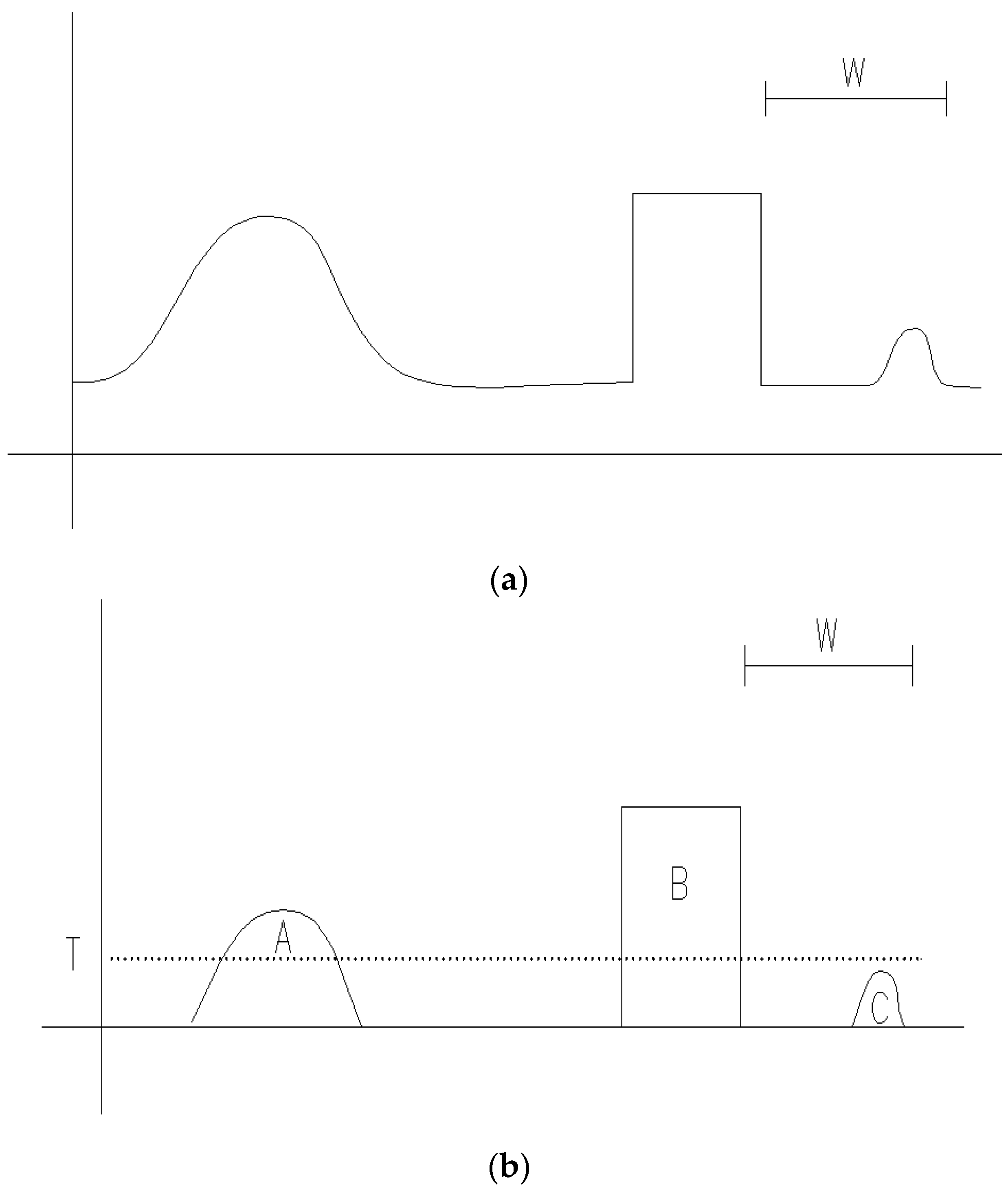
Figure 1a illustrates an area with protruding terrains. When morphological filtering with filtering window
W is applied, a result like shown in
Figure 1b can be obtained. From
Figure 1b, it can be seen that building B is completely removed while small protruding terrain C is preserved with elevation difference threshold for
T. However, the larger protruding terrain A is removed as object, which would make the final result have larger omission error. Therefore, a conclusion to be drawn here is that traditional morphological filtering algorithms have challenges in determining whether the height differences are caused by protruding terrain or by objects, especially when using large filtering windows.
In order to suppress the omission error caused by protruding terrain, this paper improved the traditional progressive morphological filtering algorithm. Although protruding terrain and objects both have elevation-jump, for the region as a whole, the terrain slope gradient of the DTM in the location of protruding terrain is greater than that of the DTM in the location of object. The terrain slope gradient can be obtained by the DTM’s dilation result minus the original DTM. This can be represented in Equation (1) as [
24]:
where,
is the terrain slope gradient,
is the morphological dilation result of DTM with 3 × 3 filtering window.
Figure 1.
Example of traditional morphological filtering algorithm for removing non-ground points: (a) original point cloud; and (b) filtering results with threshold T.
Figure 1.
Example of traditional morphological filtering algorithm for removing non-ground points: (a) original point cloud; and (b) filtering results with threshold T.
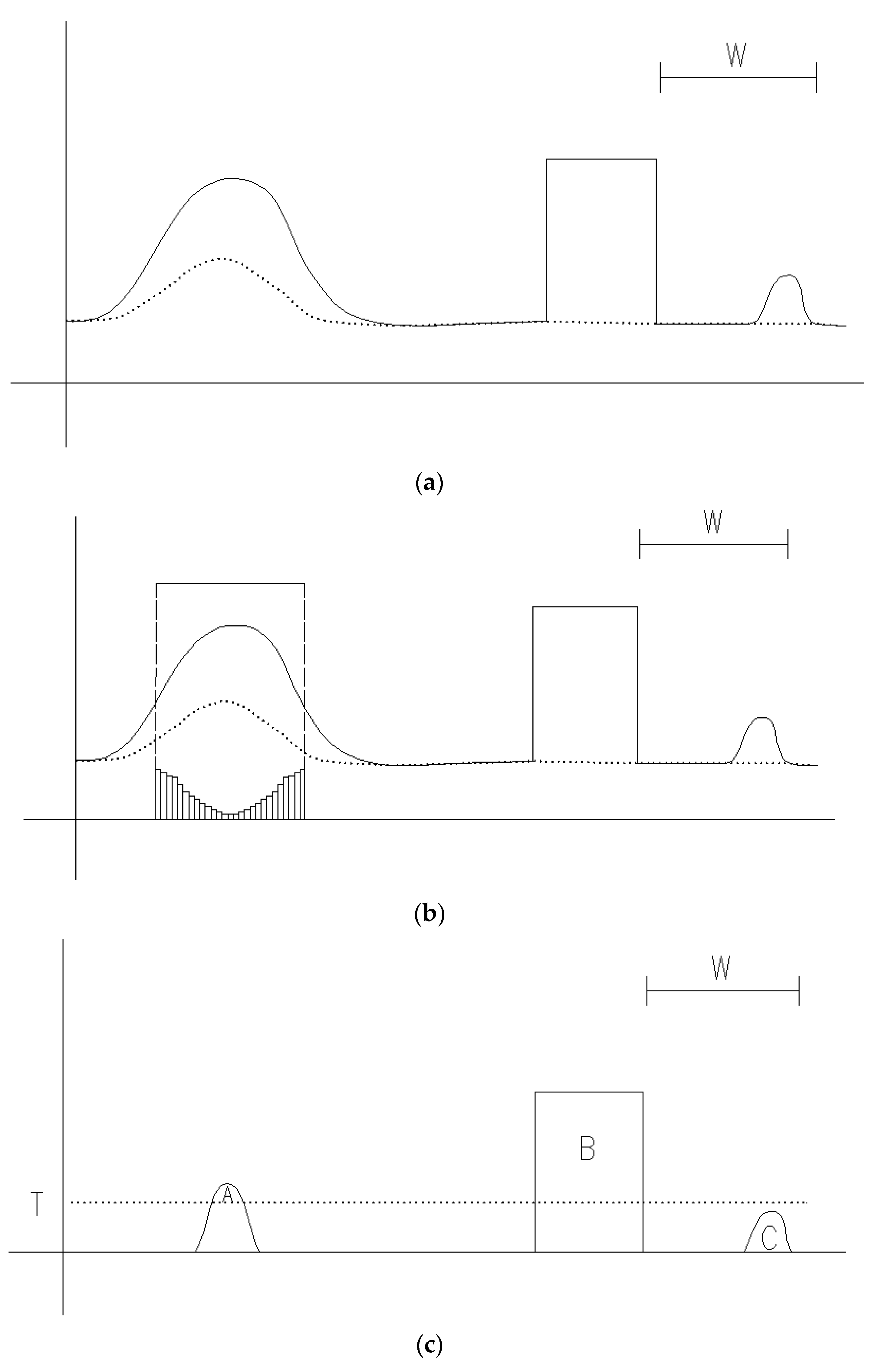
From Equation (1), it can be seen that to calculate the terrain slope gradient, the DTM should be obtained first. The DTM can be gotten by interpolating with points with local minimum elevation value under the window
, as shown in
Figure 2a. The morphological dilation operation can then be performed to the DTM, and the terrain slope gradient calculated, as shown in
Figure 2b. The final filtering results (
Figure 2c) can be obtained using the morphological filtering results in
Figure 1b minus the terrain slope gradient in
Figure 2b. With reference to
Figure 2c, it can be found that compared with the results in
Figure 1b, the misjudgment area
A reduces much while the building B is still removed and the small protruding terrain
C is still preserved. Therefore, it can be seen that the proposed method not only retains the filtering effect of the traditional progressive morphological filtering algorithm, but also reduces the misjudgment of protruding terrain and preserves terrain details as much as possible.
Figure 2.
Example of working flow of the proposed method: (a) original point cloud (solid line) and interpolated surface (dotted line); (b) the terrain slope gradient (small rectangles); and (c) filtering results.
Figure 2.
Example of working flow of the proposed method: (a) original point cloud (solid line) and interpolated surface (dotted line); (b) the terrain slope gradient (small rectangles); and (c) filtering results.
3. Implementation Steps
It is important to note that the proposed algorithm is a type of progressive multi-level method just like in [
14]. However, a distinction between the two methods is that, the present study algorithm is based on morphology while the interpolation method was only applied to calculate the slope gradient to suppress omission errors in protruding terrain.
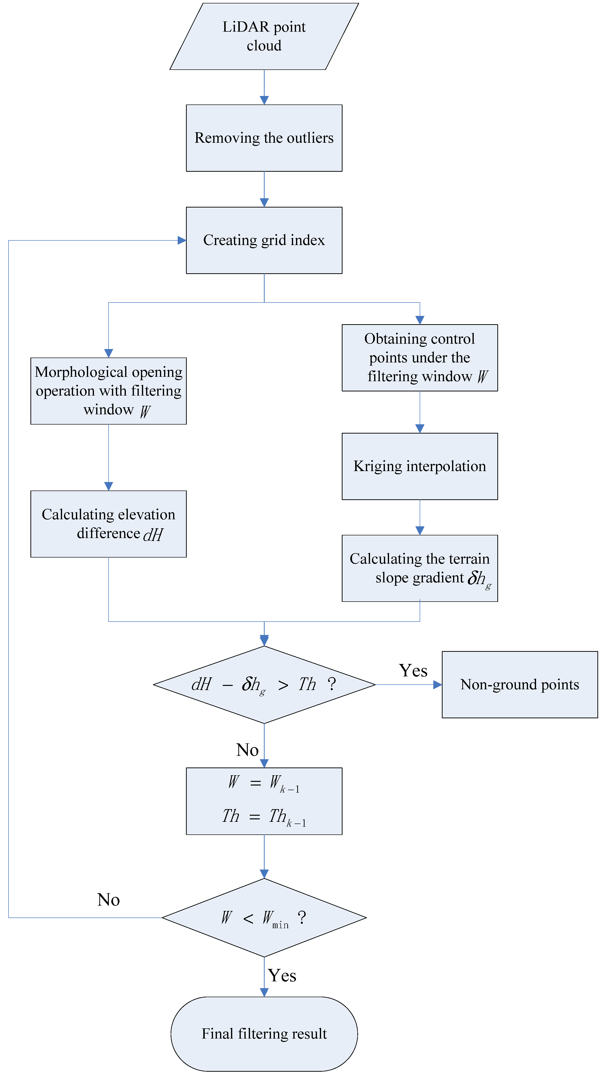
The filtering window is downsized gradually in a top-to-bottom fashion with the largest window slightly larger than the largest object in the landscape. Firstly, a grid index of the point cloud was created. Morphological filtering was then conducted to the grid cell organized data under the filtering window
W, and the differences in elevation
dH between the two successive filtered surfaces was calculated. At the same time, the reference surface of this level was interpolated with points having minimum elevation under the current window
W using a kriging method. The terrain slope gradient
δhg was then estimated using morphological dilation to the reference surface. Finally, the difference value of elevation difference
dH and terrain slope gradient
δhg was calculated to know whether the point is an object point or ground point. It is worth mentioning that if
dH is greater than
Th, the point will be classified as object and removed. On the other hand, if
dH is less than
Th, the point will be classified as ground point and preserved to do the next level’s operation. When this level’s filtering is done, the filtering window size decreases and elevation difference threshold
Th changes accordingly. This level’s filtering results were used to create new grid index. This process iterates until the window size
W is not larger than the preset minimum window size
Wmin. The flow chart of this proposed algorithm is shown in
Figure 3. The improved algorithm is mainly composed of the following five steps.
Figure 3.
Flow chart of the proposed method.
Figure 3.
Flow chart of the proposed method.
3.1. Creating Grid
To manage irregular point cloud, a grid
was created. Point cloud was first partitioned in XY-plane according to the preset cell size.
f(p) is the value of
f at p, which is selected as the lowest point within the corresponding cell [
24]. If a cell contains no point, it is assigned the value of the nearest point.
3.2. Removing Low Outliers
Low outliers originate from multi-path errors and errors in the laser range finder [
26]. As most filters work on the assumption that the lowest points in a point cloud must belong to terrain [
26], it is important to remove these low outliers first. This is because low outliers have no regularity and therefore impossible to accurately remove all low outliers without manual intervention. Consequently, the method of removing low outliers in this paper involved two steps:
(i) The denoising window was set based on point cloud partition result to 3 × 3. The low outliers were then removed based on the elevation point values within the denoising window. However, the elevation point values less than the minimum elevation threshold
were seen as low outliers. The minimum elevation threshold is defined in Equation (2) as:
where,
is the mean value of all elevation points within window, and
is the corresponding standard deviation.
(ii) The low outliers detected in the first step were then manually corrected.
3.3. Morphological Opening Operation
Morphological opening operation applied to point cloud consists of erosion operation followed by dilation operation. In the morphological erosion operation
Ew(
f) the smallest value of all points within the window was selected, while in the dilation operation
Dw(
f) the largest value of all points within the window was chosen. The morphological opening operation
Ow(
f) could be defined in Equation (3) as:
The elevation difference
between the morphological opening operation before and after was calculated using Equation (4):
3.4. Kriging Interpolation
Kriging interpolation is an unbiased and optimal estimation method by using known variables and structure features of the variogram [
27]. Assuming that the unknown point p is around several known sample points, namely
and their corresponding sample values are
f(p), (
). The estimation value of the unknown point
can be calculated according to ordinary kriging interpolation using Equation (5) [
27]:
where,
is the weight which denotes each of the samples’ proportion to the calculation of the unknown point.
As can be seen from Equation (5), if weight 𝜆
i is known, the estimation value of the unknown point can be calculated. Kriging interpolation is unbiased and has least variance. Its mean and variance are given in Equation (6) [
27] as:
Equation (6) denoted by variogram can be computed using the Lagrange multiplier method [
27]:
Equation (7) can also be written in matrix form [
27] as:
where
is the variogram, and 𝜆
i is the weight.
From Equations (9) and (10), in order to determine the weight 𝜆, the variogram
should be calculated first. This paper selected the spherical model as the theoretical variogram. This was selected because the spherical model shows the spatial correlation between an unknown point and the known point decreases when the distance between them increases. When the distance is greater than a certain value, the spatial correlation is zero. These characteristics meet the DTM interpolation requirement. The general form of spherical variogram [
27] can be expressed as:
where,
is nugget,
c is spatial variance,
h is lag distance, and
a is range.
Least squares method can be employed to fit the above model by using known sample points, and subsequently the coefficients of the spherical variogram model can be obtained. In this paper, the known sample points are points with the lowest elevation values referred to as control points found within the filtering window
W of the current hierarchy [
14]. Because the largest filtering window
W is larger than the largest object in the region, it is obvious that the control points obtained within the filtering window could be seen as ground points. Hence, the largest objects are removed and the window size is decreased. Thus, in the next hierarchy, the new control points obtained under the new window can also be seen as ground points. Therefore, the reference surface interpolated by kriging method using these control points can be seen as DTM. Moreover, the precision of the DTM could become better and better. After obtaining the DTM, the terrain slope gradient
δhg can be calculated using Equation (1).
3.5. Filtering Judgment
At each hierarchy, the elevation difference dH of the point between the morphological opening operation before and after can be calculated. If the difference between dH and δhg is greater than the threshold Th, this point will be classified as non-ground point and removed.
4. Experimental Comparison
This paper used a benchmark dataset provided by the ISPRS commission to test the performance of the proposed method. This benchmark dataset is collected with an Optech ALTM scanner and located in the Vaihingen/Enz test field and Stuttgart city center. The benchmark dataset consists of 15 samples with the average point-spacing of 1.0–1.5 m in urban areas (from S11 to S42) and 2.0–3.5 m in the rural areas (from S51 to S71). These samples cover diverse feature contents, such as large buildings, low vegetation, and steep slopes among others [
26]. Moreover, for each sample, the reference data is provided by semi-automatic filtering and manual editing with knowledge of the landscape and available aerial images [
25].
Four accuracy indexes namely omission error, commission error, total error and kappa coefficient were used to access the filtering effect of the proposed method in this paper. Omission error also referred to as type I error is the percentage of ground points rejected as non-ground points in all ground points; while commission error known as type II error refers to the percentage of non-ground points accepted as ground points in all non-ground points. Total error on the other hand is the percentage of incorrectly classified points in all points. Kappa coefficient is an alternative measure of the overall classification accuracy that subtracts the effect of chance agreement and quantifies how much better a particular classification is, as compared with a random classification [
15].
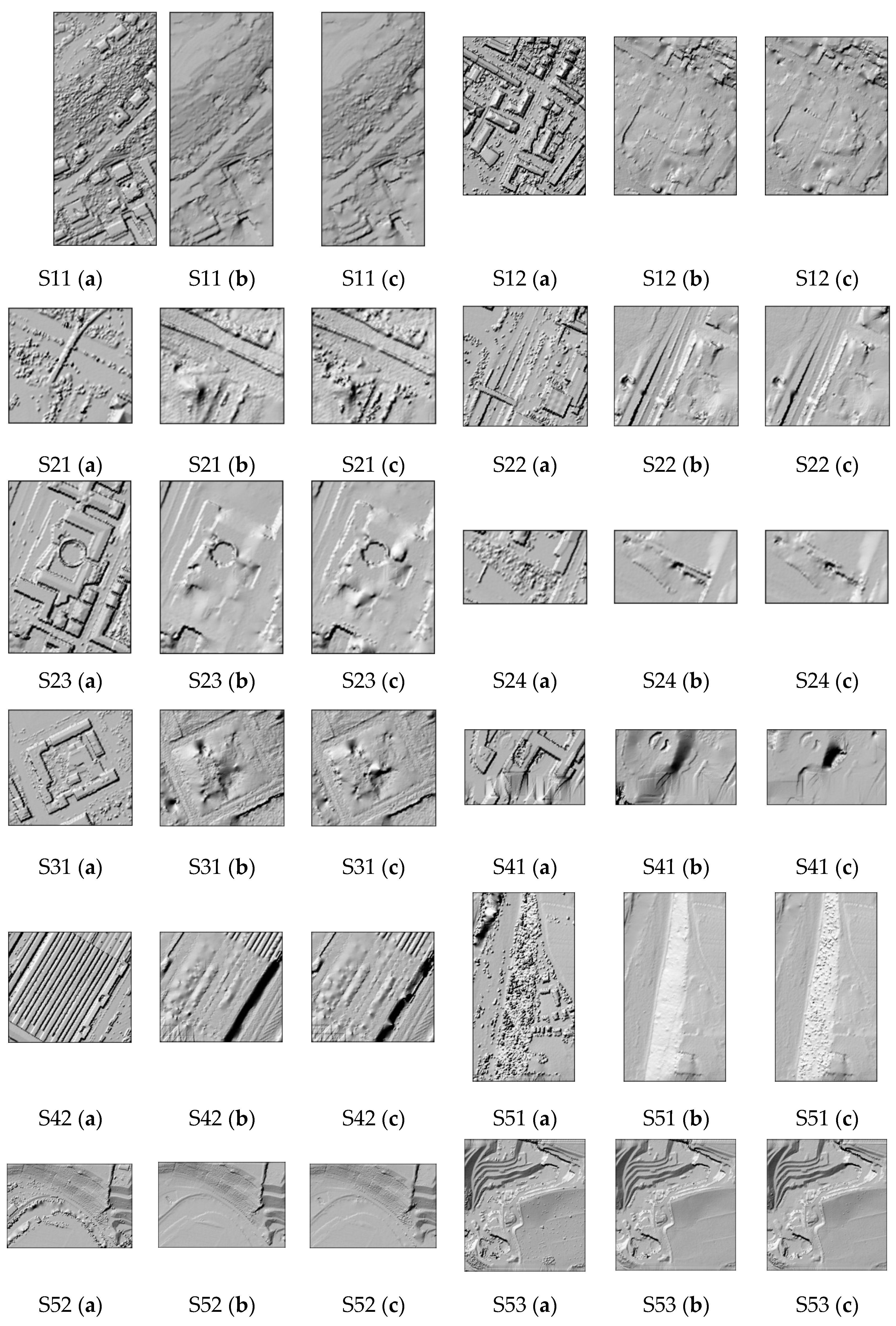
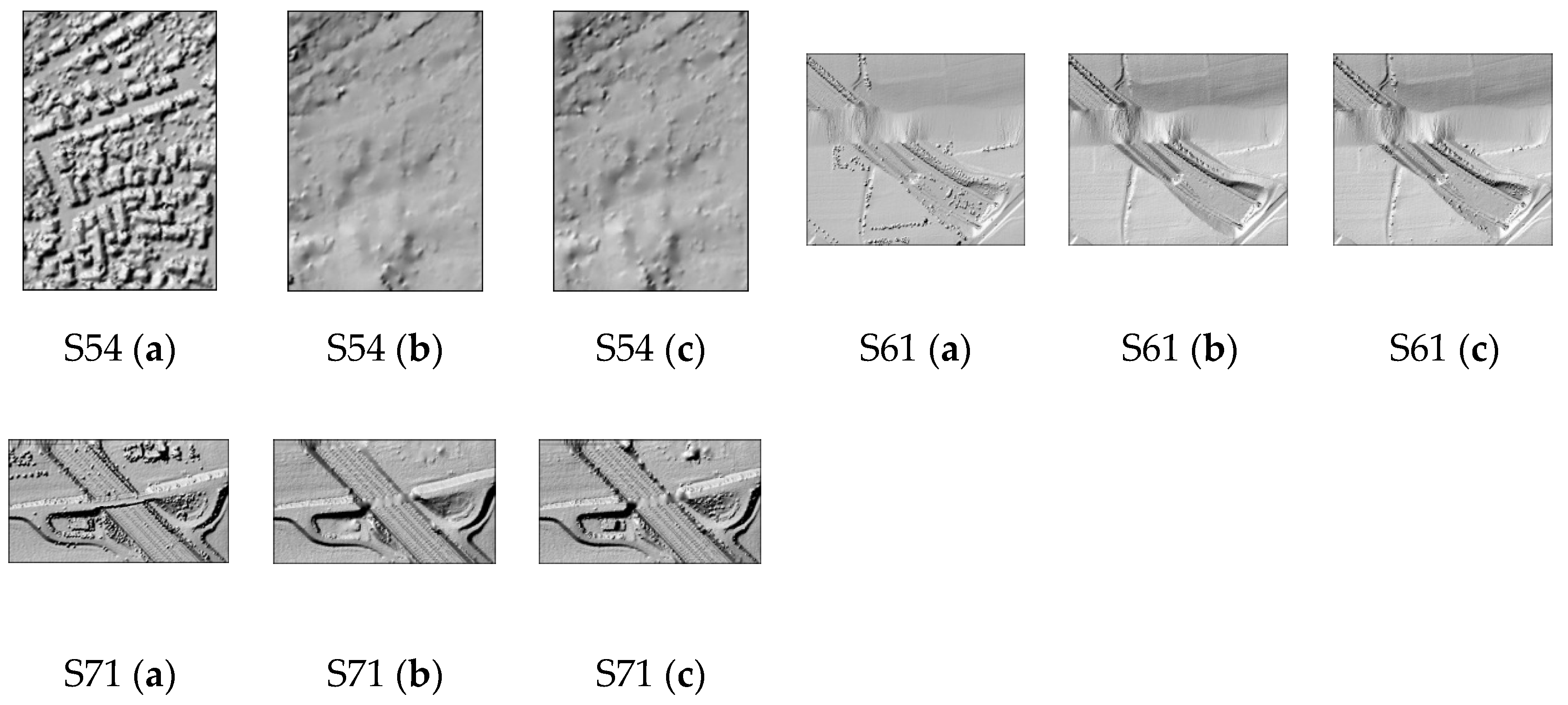
The results obtained from the various accuracy indexes are presented in
Table 1. To intuitively access the filtering effects, (a) the original digital surface model (DSM) generated from the raw point cloud; (b) the true digital elevation model (DEM) generated from the true ground points; and (c) the filtered DEM generated from the ground points derived by our filtering algorithm are shown in
Figure 4.
Table 1 shows that five samples, namely S12, S21, S31, S42, and S54 had a kappa coefficient more than 90% and total error less than 5%. This assertion is corroborated in
Figure 4 that the aforementioned five sample areas were all relatively flat and terrain slope changes slightly. This is consistent with the conclusion of the existing algorithms that filtering methods works well in fairly flat terrain but become less reliable as the slope of the terrain increases [
28]. The total error of S11 and S41 are both more than 10%.
Figure 4 indicates that sample S11 has greater slope change and many buildings are built on steep slopes. Besides, there are lots of low vegetation on the slope which was accepted as ground points. Whereas many low outliers were hard to remove in S41. From S41 (b) and S41 (c) in
Figure 4, it was observed that the filtered DEM of sample S41 has a bigger deviation with the true DEM. Thus, further confirming the assertion that the final filtering results are influenced by low outliers [
26]. In terms of the kappa coefficient, the proposed method had the poorest classification results for sample S53 because of the existence of many elevation-jump areas. In order to preserve more terrain details, the typeⅡerror was more than 20% for sample S53 with a total error less than 10% (
Table 1). In the case of samples S61 and S71, the typeⅡerror more than 20% was attained. The reason for this is that these two areas have much low vegetation. Conversely, their type I error and total error were both smaller.
Table 1.
Accuracy indexes for all sample dataset.
Table 1.
Accuracy indexes for all sample dataset.
| Sample | Type I | Type II | Total | Kappa |
|---|
| Dataset | (%) | (%) | (%) | (%) |
| S11 | 13.63 | 12.96 | 13.34 | 72.92 |
| S12 | 4.86 | 2.08 | 3.50 | 93.00 |
| S21 | 0.01 | 9.95 | 2.21 | 93.35 |
| S22 | 5.27 | 5.74 | 5.41 | 87.58 |
| S23 | 4.00 | 6.35 | 5.11 | 89.74 |
| S24 | 7.47 | 7.48 | 7.47 | 81.93 |
| S31 | 0.87 | 1.86 | 1.33 | 97.33 |
| S41 | 18.17 | 3.07 | 10.60 | 78.78 |
| S42 | 3.04 | 1.45 | 1.92 | 95.38 |
| S51 | 1.42 | 17.25 | 4.88 | 85.06 |
| S52 | 5.59 | 14.86 | 6.56 | 69.51 |
| S53 | 6.78 | 23.90 | 7.47 | 41.84 |
| S54 | 4.90 | 3.52 | 4.16 | 91.63 |
| S61 | 1.54 | 24.54 | 2.33 | 67.82 |
| S71 | 0.96 | 25.42 | 3.73 | 79.86 |
| Ave | 5.23 | 10.70 | 5.33 | 81.72 |
Figure 4.
Filtering results: (a) the DSMs before filtering; (b) the true DEMs generated from the true ground points; and (c) the filtered DEMs generated from the ground points derived by the proposed filtering algorithm.
Figure 4.
Filtering results: (a) the DSMs before filtering; (b) the true DEMs generated from the true ground points; and (c) the filtered DEMs generated from the ground points derived by the proposed filtering algorithm.
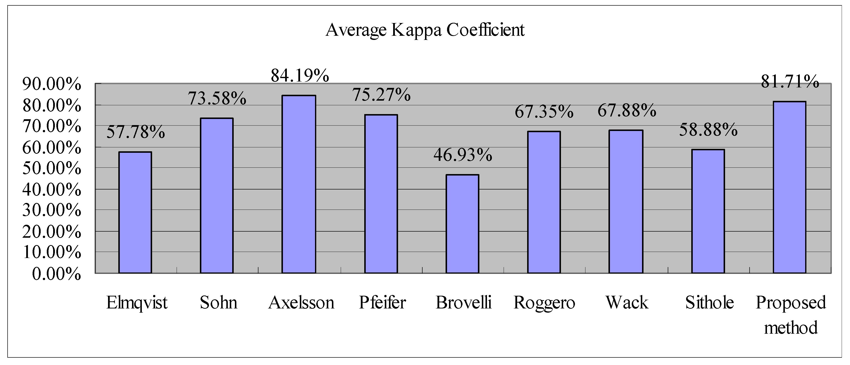
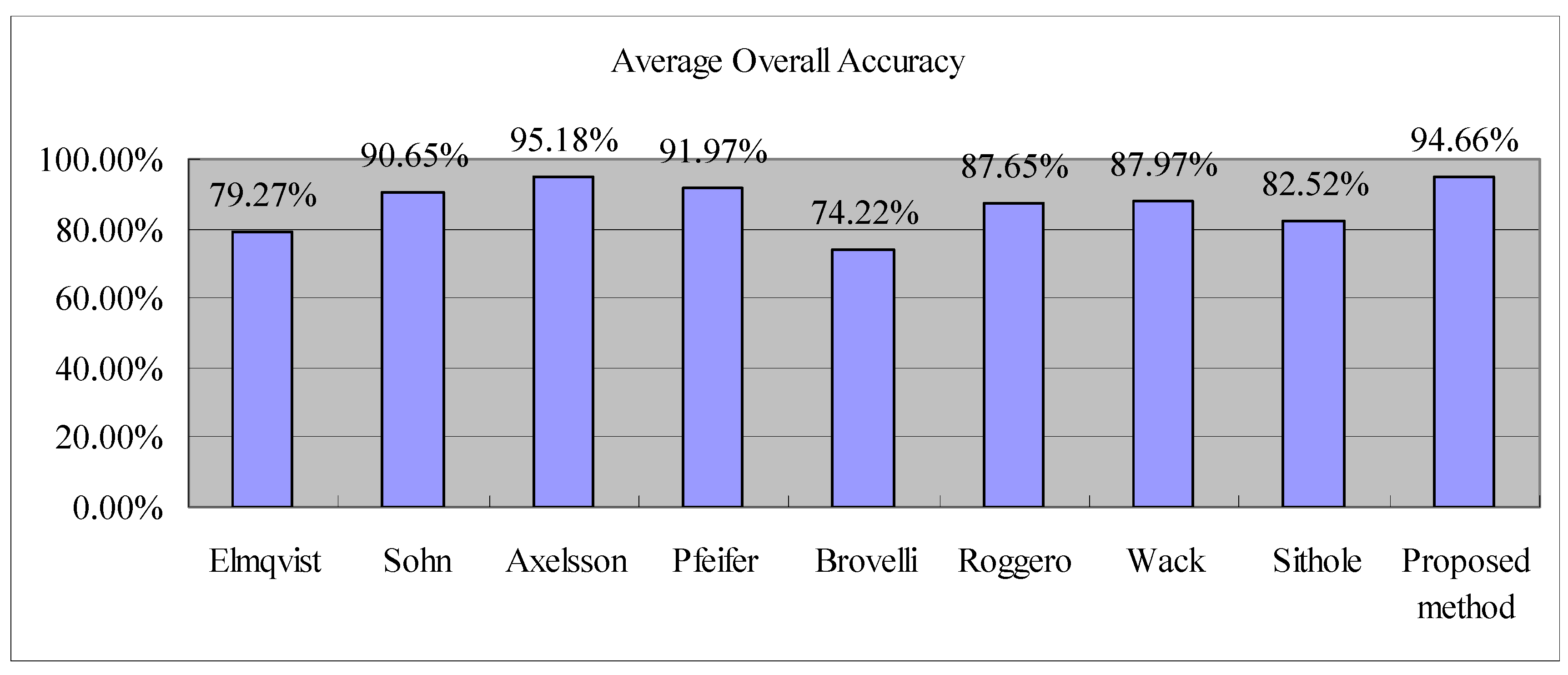
Table 1 and
Figure 4 show the filtering accuracy and filtering effect of the proposed method respectively. To objectively evaluate the merits of the proposed method, this paper compared the filtering results of the proposed method to eight other algorithms tested by the ISPRS [
28]. The comparison results are shown in
Figure 5 and
Figure 6. The precision evaluation indexes are the average kappa coefficient and the average overall accuracy of the 15 samples. The overall accuracy refers to the percentage of correctly classified points in all points. By visual inspection of
Figure 5 and
Figure 6, it can be observed that the accuracy of the proposed method is only 2.48% lower than that of Axelsson method. This is because results of the proposed method for three samples namely S52, S53 and S61 had kappa coefficient lower than 70%, which make the final average kappa coefficient slightly lower. Three methods (Sohn [
9], Pfeifer [
12], and Axelsson [
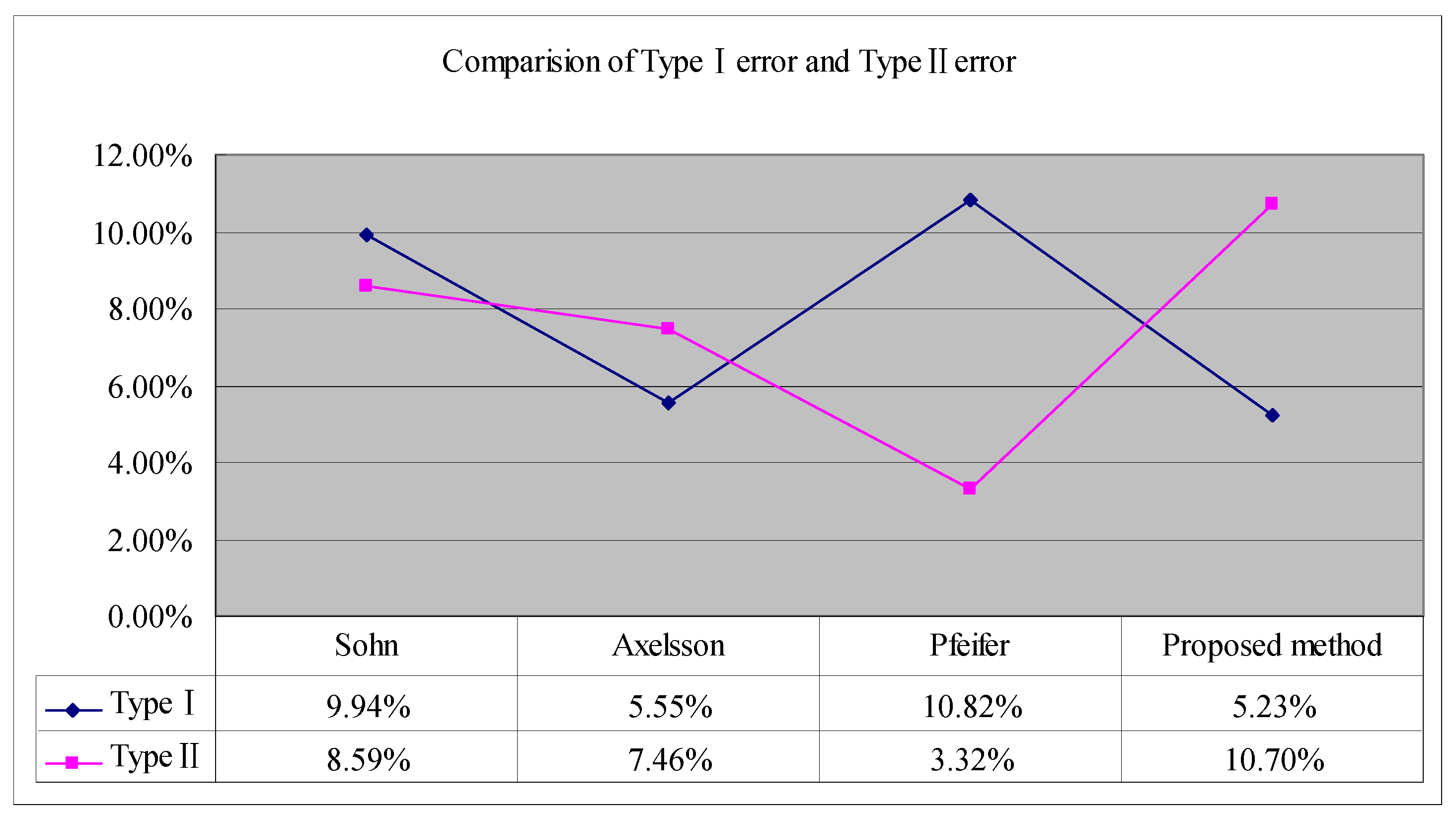
13]) with high kappa coefficient and overall accuracy were identified to have comparable average typeⅠerror and average typeⅡerror with the ones of the proposed method. As shown in
Figure 7, the average typeⅠerror of the proposed method is the lowest, but the average typeⅡerror is the highest. This is because the typeⅡerrors of samples S51, S53, S61 and S71 are too high making the final average typeⅡerror to be highest among the four methods. In view of this, a conclusion can be drawn that, typeⅡerror tends to increase with the decrease of type I error.
Figure 5.
Comparison of average kappa coefficient of the different filtering algorithms.
Figure 5.
Comparison of average kappa coefficient of the different filtering algorithms.
Figure 6.
Comparison of average overall accuracy of the different filtering algorithms.
Figure 6.
Comparison of average overall accuracy of the different filtering algorithms.
Figure 7.
Comparison of average type I error and average type II error of the four filtering algorithms.
Figure 7.
Comparison of average type I error and average type II error of the four filtering algorithms.
The total errors of the 15 samples for the proposed method and the eight classical filtering algorithms are shown in
Table 2. The proposed method obtained the lowest total error for samples S21, S31, and S53, whereas the total errors of the remaining samples are close to the corresponding lowest total errors. Although the average total error of the proposed method is 2.51% higher than that of Axelsson’s method [
13], the proposed method performs much better in areas with complex buildings, such as S21 and S31 with the total error 2.21% and 3.45% lower than that of Axelsson’s method [
13]. Furthermore, the proposed method also obtains the best filtering result in the area with many terrain discontinuities, such as S53. Thus, a conclusion can be drawn here is that the proposed method can perform well in most terrain environments, especially in areas with complex buildings or terrain discontinuities.
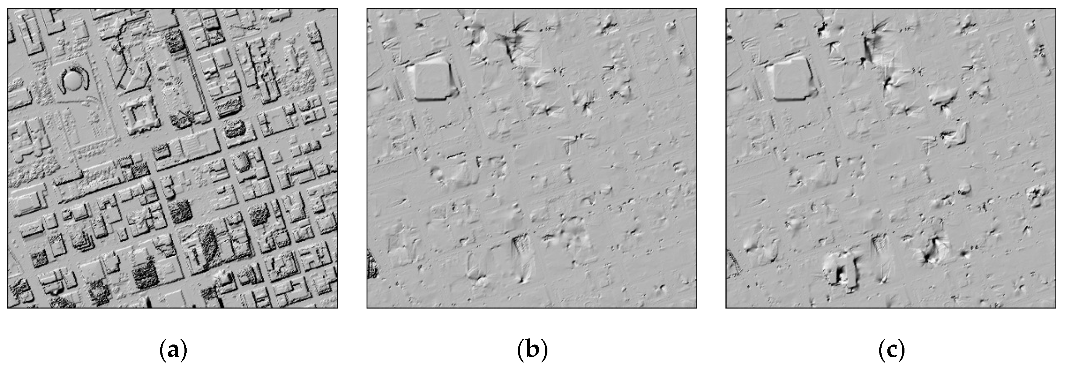
Another dataset used in practice was tested to evaluate the performance of the proposed method. The new dataset is located in Taiyuan, China with an average point density of 6 points/m
2. It is important to know that diverse terrain features such as complex buildings, low vegetation,
etc. (
Figure 8a), are covered in Taiyuan, China. True ground points were manually classified from original point cloud for accuracy evaluation (
Figure 8b). Filtering result is shown in
Figure 8c. Type I, type II and total errors are 0.75%, 1.80%, and 1.25%, respectively. It can be found that the performance of the proposed method is quite well, which also confirmed that the proposed method suits well in urban areas, where many buildings with complex structures and shapes existed.
Table 2.
Comparison of total errors of the proposed method and the eight classical filtering for all study samples (the bold value is the smallest one in each line).
Table 2.
Comparison of total errors of the proposed method and the eight classical filtering for all study samples (the bold value is the smallest one in each line).
| Samples | Elmqvist | Sohn | Axelsson | Pfeifer | Brovelli | Roggero | Wack | Sithole | Proposed Method |
|---|
| (%) | (%) | (%) | (%) | (%) | (%) | (%) | (%) | (%) |
|---|
| S11 | 22.4 | 20.49 | 10.76 | 17.35 | 36.96 | 20.8 | 24.02 | 23.25 | 13.34 |
| S12 | 8.18 | 8.39 | 3.25 | 4.5 | 16.28 | 6.61 | 6.61 | 10.21 | 3.5 |
| S21 | 8.53 | 8.8 | 4.25 | 2.57 | 9.3 | 9.84 | 4.55 | 7.76 | 2.21 |
| S22 | 8.93 | 7.54 | 3.63 | 6.71 | 22.28 | 23.78 | 7.51 | 20.86 | 5.41 |
| S23 | 12.28 | 9.84 | 4 | 8.22 | 27.8 | 23.2 | 10.97 | 22.71 | 5.11 |
| S24 | 13.83 | 13.33 | 4.42 | 8.64 | 36.06 | 23.25 | 11.53 | 25.28 | 7.47 |
| S31 | 5.34 | 6.39 | 4.78 | 1.8 | 12.92 | 2.14 | 2.21 | 3.15 | 1.33 |
| S41 | 8.76 | 11.27 | 13.91 | 10.75 | 17.03 | 12.21 | 9.01 | 23.67 | 10.6 |
| S42 | 3.68 | 1.78 | 1.62 | 2.64 | 6.38 | 4.3 | 3.54 | 3.85 | 1.92 |
| S51 | 23.31 | 9.31 | 2.72 | 3.71 | 22.81 | 3.01 | 11.45 | 7.02 | 4.88 |
| S52 | 57.95 | 12.04 | 3.07 | 19.64 | 45.56 | 9.78 | 23.83 | 27.53 | 6.56 |
| S53 | 48.45 | 20.19 | 8.91 | 12.6 | 52.81 | 17.29 | 27.24 | 37.07 | 7.47 |
| S54 | 21.26 | 5.68 | 3.23 | 5.47 | 23.89 | 4.96 | 7.63 | 6.33 | 4.16 |
| S61 | 35.87 | 2.99 | 2.08 | 6.91 | 21.68 | 18.99 | 13.47 | 21.63 | 2.33 |
| S71 | 34.22 | 2.2 | 1.63 | 8.85 | 34.98 | 5.11 | 16.97 | 21.83 | 3.73 |
| Ave | 20.87 | 9.35 | 4.82 | 8.02 | 25.78 | 12.35 | 12.04 | 17.48 | 5.33 |
Figure 8.
Filtering result: (a) the DSM before filtering; (b) the true DEM generated from the true ground points; and (c) the filtered DEM generated from the ground points derived by the proposed filtering algorithm.
Figure 8.
Filtering result: (a) the DSM before filtering; (b) the true DEM generated from the true ground points; and (c) the filtered DEM generated from the ground points derived by the proposed filtering algorithm.
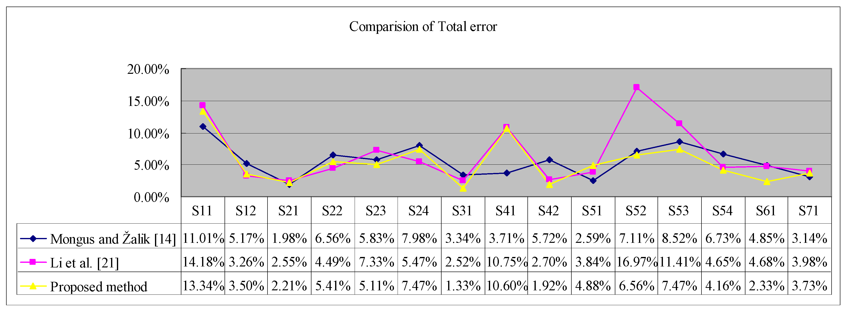
The proposed method in the present study is related to the multi-level interpolation method proposed by Mongus and Žalik [
14] and the morphological filtering algorithm proposed by Li
et al. [
21]. The comparison of the total error of the three methods against the 15 samples is shown in
Figure 9. The proposed method obtained the lowest total errors for 7 out of 15 samples, including S23, S31, S42, S52, S53, S54 and S61. Among the seven samples, S52, S53, and S61 had protruding terrain features and the proposed method’s total errors of these three samples are all lower than that of the other two methods. Thus, it can be seen that the proposed method has significant advantage in protecting terrain details hence realizing the purpose of the improved algorithm.
In recent years, several researchers have proposed their respective new filtering algorithms and used the 15 samples provided by the ISPRS to evaluate their performance. The average total errors of these filtering algorithms are summarized in
Table 3. The Results showed that the proposed method performed better than most of these algorithms, but the average total error was still 2.59% higher than the lowest one. This can be explained by the nature of the morphological filtering. Morphology-based filtering algorithms will not suite well for steep terrain with dense vegetation on top, such as sample S11. In this case, the suppressing omission error method introduced in this paper will not work so well and it will be hard to identify discrete objects to be removed by morphological filtering, since brush and trees are mixed up with the DTM in a fractal fashion.
Figure 9.
Comparison of the total error of different filtering algorithms for all samples.
Figure 9.
Comparison of the total error of different filtering algorithms for all samples.
Table 3.
Comparison of average total errors of the proposed method and other ten filtering algorithms proposed in recent years.
Table 3.
Comparison of average total errors of the proposed method and other ten filtering algorithms proposed in recent years.
| Author | Total (%) |
|---|
| Chen et al. [18] | 7.23 |
| Jahromi et al. [29] | 7.70 |
| Mongus and Žalik [14] | 5.62 |
| Susaki [11] | 7.39 |
| Chen et al. [15] | 4.11 |
| Pingel et al. [30] | 4.40 |
| Li et al. [20] | 6.19 |
| Mongus et al. [24] | 2.74 |
| Li et al. [21] | 6.58 |
| Li et al. [22] | 6.73 |
| Proposed method | 5.33 |


