Mapping Complex Urban Land Cover from Spaceborne Imagery: The Influence of Spatial Resolution, Spectral Band Set and Classification Approach

Abstract

Detailed land cover information is valuable for mapping complex urban environments. Recent enhancements to satellite sensor technology promise fit-for-purpose data, particularly when processed using contemporary classification approaches. We evaluate this promise by comparing the influence of spatial resolution, spectral band set and classification approach for mapping detailed urban land cover in Nottingham, UK. A WorldView-2 image provides the basis for a set of 12 images with varying spatial and spectral characteristics, and these are classified using three different approaches (maximum likelihood (ML), support vector machine (SVM) and object-based image analysis (OBIA)) to yield 36 output land cover maps. Classification accuracy is evaluated independently and McNemar tests are conducted between all paired outputs (630 pairs in total) to determine which classifications are significantly different. Overall accuracy varied between 35% for ML classification of 30 m spatial resolution, 4-band imagery and 91% for OBIA classification of 2 m spatial resolution, 8-band imagery. The results demonstrate that spatial resolution is clearly the most influential factor when mapping complex urban environments, and modern “very high resolution” or VHR sensors offer great advantage here. However, the advanced spectral capabilities provided by some recent sensors, coupled with contemporary classification approaches (especially SVMs and OBIA), can also lead to significant gains in mapping accuracy. Ongoing development in instrumentation and methodology offer huge potential here and imply that urban mapping opportunities will continue to grow.

1. Introduction

Detailed land cover information is crucial for mapping and managing complex urban environments across local and regional scales [1,2], and remote sensing is the only practical and cost-effective means of generating such information over large areas [3]. However, mapping urban land poses a significant challenge for remote sensing due to the high spatial frequency of surface features [4,5,6]; urban land is highly heterogeneous, involving a mosaic of both human-made materials (such as asphalt, concrete, roof tiles and other impervious surfaces) and semi-natural surfaces (for instance grass, trees, bare soil, water etc.). Therefore, although spaceborne remote sensing has been employed for urban land cover classification over several decades, early work was limited by the relatively coarse spatial resolution of available sensors, perhaps most commonly Landsat Thematic Mapper (TM) and its 30 m resolution multispectral imagery [7,8]. In urban environments, this level of spatial detail leads inevitably to mixed pixels, whereby each pixel exhibits some spectral average representing multiple surface features [9,10,11].

1.1. VHR Sensors

A breakthrough for urban mapping came around the turn of the millennium with the advent of so-called “very high resolution” (VHR) satellite sensors, led by the 4 m spatial resolution (multispectral) IKONOS mission in 1999, but followed by a series of other instruments including OrbView-3 (also 4 m resolution), QuickBird (2.4 m) and GeoEye-1 (1.6 m) [12]. The advantage of these image sources for classifying urban land cover is obvious; the fine spatial resolution enables relatively accurate identification of small urban features [13,14,15]. Nonetheless, despite their benefit of fine spatial resolution, these VHR instruments tended to have rather limited spectral capabilities. For instance, compared with Landsat TM’s seven spectral bands (three visible, near infrared, two shortwave infrared and thermal infrared), IKONOS, OrbView-3, QuickBird and GeoEye-1 each has only four (visible and near infrared) spectral bands. Such a limited spectral band set potentially constrains the ability of remotely sensed imagery to distinguish between urban surfaces, given their often subtly varying spectral properties [4,16]. This is perhaps especially a problem where detailed thematic classification is attempted (i.e., where many specific land cover classes are mapped rather than few broad categories). For instance, a planning agency official conducting a land use inventory may wish to map several different types of roofing materials rather than a single “buildings” class [17].

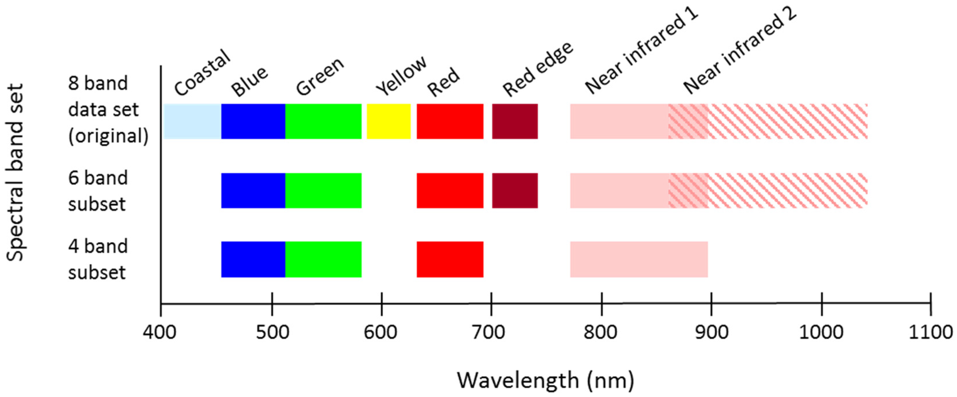
1.2. Enhanced Spectral Capabilities

Now, a latest generation of satellite sensors is emerging with enhanced spectral, as well as advanced spatial, properties. Notably, two new VHR instruments, WorldView-2 (WV2) and WorldView-3 (WV3), acquire multispectral imagery with eight spectral bands: coastal, blue, green, yellow, red, red-edge, near infrared 1 (NIR1) and near infrared 2 (NIR2). In particular, the coastal, yellow and red-edge bands, as well as NIR2, represent “new” spectral bands, not routinely found on multispectral sensors. (Indeed, these advancements in spectral capability are not restricted to VHR instruments; the most recent Landsat sensor, Operational Land Imager (OLI), has ten multispectral bands, including new coastal, cirrus and thermal infrared 2 bands.) These enhanced spectral properties may prove especially valuable for urban mapping, enabling subtly varying spectral classes to be identified [18]. This advantage is likely to be most pertinent where detailed classification schema are involved, for instance when identifying many different land cover classes in complex urban environments.

1.3. Pixel-Based versus Object-Based Classification

Notwithstanding these spectrally and spatially advanced satellite sensors, difficulties remain for urban mapping. Traditionally, urban classification has been conducted using pixel-based approaches, whereby land cover classes are allocated to each individual pixel [18,19]; and historically most such analysis has employed statistical parametric classifiers such as the maximum likelihood (ML) algorithm [15,20,21]. Though ML classification is a perfectly valid method, it makes certain statistical assumptions about the data, and the nature of VHR imagery can mean that it is difficult to honour these assumptions. Specifically, ML classification tends to work well where training data are relatively “clean”, such as where coarse spatial resolution imagery is used to classify general land cover classes. Where training data are rather noisier, such as where fine resolution imagery is used to map complex, e.g., urban, environments, the ML classifier can be considerably less accurate [9,21]. More generally, pixel-based approaches as a whole have limitations when it comes to urban analysis using VHR imagery [21,22]. Contrary to the problem of mixed pixels which occurs where image spatial resolution is too coarse, VHR imagery can effectively “over-sample” the scene whereby within-feature variation (occurring where image resolution is too fine) reduces pixel-based classification accuracy [5,23,24,25].

Recent years have seen significant development with classification methodologies, and some of these have particular relevance for urban mapping. Non-parametric pixel-based classifiers such as support vector machines (SVMs) seem well-suited to VHR urban classification since they are better able to handle noisy training data, compared to for instance the ML classifier [18,26]. Moreover, object-based classification has grown in popularity, whereby land cover classes are allocated to objects representing real-world features instead of somewhat arbitrary pixel structures [23]. Other practitioners have tested spatial indices and wavelet-based approaches to enhance classification performance [27].

The object-based approach directly addresses, and to an extent overcomes, the problem of within-feature variation and its attendant (pixel-based) misclassification [1,28,29]. Consequently, object-based classification, which exploits spatial, textural and topological (as well as spectral) information [30,31,32] may facilitate highly accurate mapping of complex urban environments using VHR imagery.

1.4. Mapping Complex Urban Land Cover

Theory underpinning spectral and spatial image properties and their influence on land cover classification accuracy is fairly well-established, and different image sources and classifiers have been tested quite widely on urban environments. However, such experiments have often tended to be limited in scope, perhaps comparing only one or two variables (e.g., spatial resolution or classification approach); and/or adopting general and unambitious thematic classification schema; and/or working with small image data sets. For instance, many studies have conducted fairly basic, procedural comparisons between pixel- and object-based classification [21,33,34], but these have not necessarily considered other influential variables such as input spatial resolution or spectral bands, or classification algorithm. Some practitioners have (sensibly) adopted VHR imagery, including WV2 data with its enhanced spectral properties, for mapping urban environments, but commonly these attempt only broad differentiation between a few general land cover classes [34,35,36] rather than detailed distinction of many specific classes. In effect, these studies seem content to replicate the sort of classification schema used for decades with medium spatial resolution imagery, rather than attempting to exploit the full information content of WV2 imagery and create very thematically-detailed urban land cover maps. Also, most test WV2 data sets tend to be very small, often only a few hectares [37], and this can limit the strength of the scientific findings since there is no consideration of spatial extrapolation or transferability of the approach. That is, the results may be very parochial and depend strongly on local context.

This paper builds on our theoretical understanding of how image and classifier characteristics influence land cover accuracy by presenting an exhaustive and rigorous practical experiment to compare the influence of spatial resolution, spectral band set and classification approach for mapping complex urban environments. Uniquely this study provides a full test of the latest VHR imagery for urban classification, demonstrating how its component (spatial and spectral) parts contribute to output mapping accuracy. Analysis is iterated using a series of different spatial resolutions and spectral band sets to simulate imagery ranging from traditional medium spatial resolution satellite sensors such as Landsat TM to state-of-the-art VHR sensors like WV2, adapting an approach developed by [38]. Moreover, given the influential role that classification approach plays on output accuracy, and how this is linked intrinsically with image specifications, all image data sets are classified using parametric and non-parametric pixel-based, and object-based, classifiers. Unlike earlier work, this study adopts a detailed classification system, including many specific land cover classes rather than few general categories. This enables a fuller and more robust assessment of the WV2 data, but also delivers helpful practical information for urban planners and other user communities on the level of thematic detail that can be achieved when mapping complex urban environments. Finally, analysis is conducted using a relatively large image covering approximately 121 km² of the city of Nottingham, UK and its environs. This means that urban land cover information is generated at a scale of practical value and relevance (the whole city-scale), unlike earlier experiments that have been limited to very small, local areas.

2. Research Materials

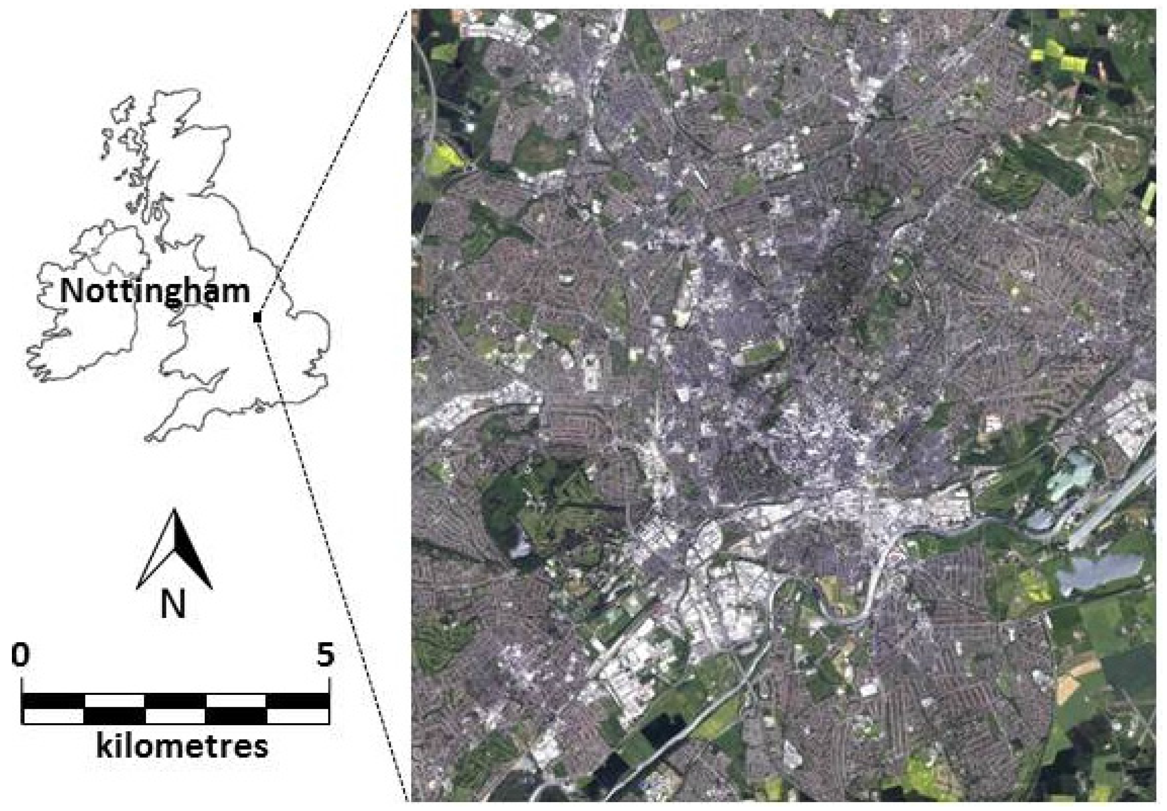
2.1. Study Area and Classification Schema

The study area is the city of Nottingham, UK and its environs (Figure 1), located at 52°57′N latitude, 1°08′W longitude. Nottingham has a population of slightly more than 300,000 [39] and covers an area of approximately 121 km². The climate is cool, moist temperate, with average high summer temperatures around 20 °C, and average monthly precipitation around 50 mm throughout the year. The topography is fairly flat, with altitude generally around 100 m. Nottingham is a relatively typical UK city, in that it comprises a mixture of residential, industrial and commercial land use, and therefore represents a good test for urban mapping methodologies. Land cover can be broadly categorised into various types of anthropogenic features (e.g., asphalt, concrete, roof materials) intersecting with the semi-natural environment (e.g., vegetation (grass, trees), bare soil and water). The central urban core is generally more built-up and less vegetated than the outlying residential areas, though this varies considerably across the city and its districts. A classification schema was developed that captured the detailed spatial heterogeneity of the urban land cover throughout Nottingham. In total, eleven classes were identified: asphalt, concrete roofs, clay roofs, slate roofs, metal roofs, grass, broadleaved trees, needle-leaved trees, bare soil, water and shadow (Table 1).

Figure 1. Nottingham, UK study area location and WorldView-2 image (© DigitalGlobe, Inc. All Rights Reserved).

Figure 1. Nottingham, UK study area location and WorldView-2 image (© DigitalGlobe, Inc. All Rights Reserved).

Table 1. Nottingham urban land cover classification schema.

Class	Description
Asphalt	Urban ground surfaces covered in asphalt such as roads and car parks
Concrete roofs	Predominantly residential buildings covered in dark grey concrete tiles
Clay roofs	Predominantly residential buildings covered in red clay tiles
Slate roofs	Predominantly residential buildings covered in light grey slate tiles
Metal roofs	Predominantly industrial buildings covered in white metal panels
Grass	Areas of grassland such as urban parks and lawns, plus surrounding rural agriculture
Broad-leaved trees	Patches of deciduous broad-leaved trees
Needle-leaved trees	Patches of evergreen needle-leaved trees
Bare soil	Open areas covered by bare soil
Water	Water bodies including lakes, rivers, ponds and canals
Shadow	Areas of shadow cast from tall structures such as buildings and trees

Table 1. Nottingham urban land cover classification schema.

Class	Description
Asphalt	Urban ground surfaces covered in asphalt such as roads and car parks
Concrete roofs	Predominantly residential buildings covered in dark grey concrete tiles
Clay roofs	Predominantly residential buildings covered in red clay tiles
Slate roofs	Predominantly residential buildings covered in light grey slate tiles
Metal roofs	Predominantly industrial buildings covered in white metal panels
Grass	Areas of grassland such as urban parks and lawns, plus surrounding rural agriculture
Broad-leaved trees	Patches of deciduous broad-leaved trees
Needle-leaved trees	Patches of evergreen needle-leaved trees
Bare soil	Open areas covered by bare soil
Water	Water bodies including lakes, rivers, ponds and canals
Shadow	Areas of shadow cast from tall structures such as buildings and trees

2.2. Image and Reference Data

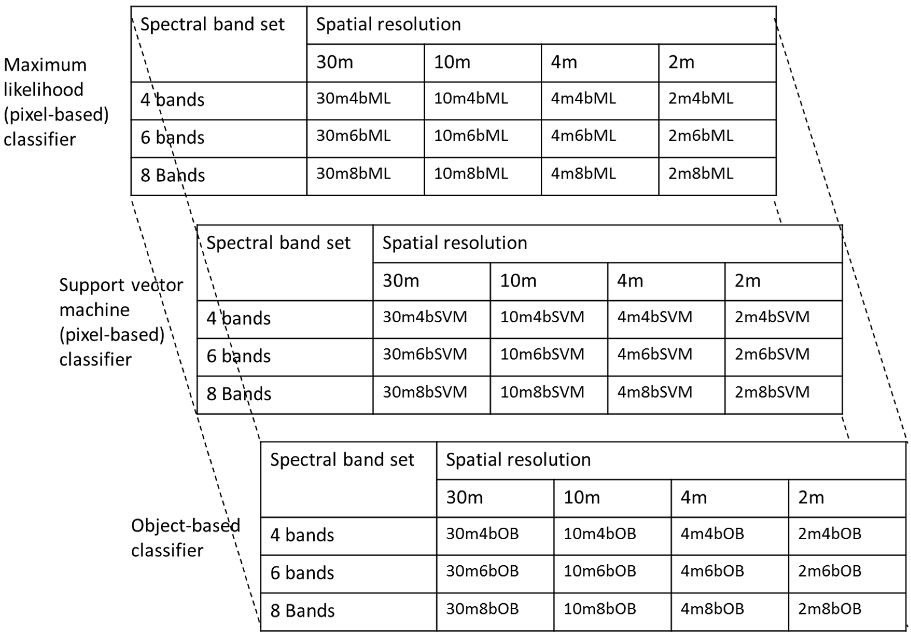
A WorldView-2 (WV2) image of Nottingham was acquired on 26 May 2012. The multispectral imagery was supplied in 11 bit data format, at a spatial resolution of 2 m and with eight spectral wavebands: coastal, blue, green, yellow, red, red edge, NIR1 and NIR2 (Figure 2, top line). Image preprocessing requirements were minimal for two reasons. First, a single source data set was used whereby all comparative outputs were derived from the original WV2 image, and this meant that geometric distortion was of relatively little consequence. Nonetheless, the image’s geometric fidelity was examined manually by cross-referencing the image with ancillary map data; geometric accuracy proved relatively high in general. Second, analysis involved thematic classification and the accuracy of output land cover maps was assessed independently (of the original spectral imagery). This meant that external factors such as atmospheric distortion that influence original (input) pixel digital numbers were of little consequence.

Figure 2. WorldView-2 spectral wavebands (top line) and spectral band subsets used for comparative analysis.

Figure 2. WorldView-2 spectral wavebands (top line) and spectral band subsets used for comparative analysis.

The original 2 m spatial resolution, 8 spectral band WV2 image was modified to create a series of spatial/spectral data sets for comparative classification analysis. First, the imagery was degraded successively to a series of coarser spatial resolutions: 4 m, 10 m and 30 m. These particular values were chosen to approximate the spatial properties of commonly used satellite sensors, ranging from state-of-the-art VHR imagery to traditional medium resolution imagery. For instance, while 2 m represents WV2, 4 m matches earlier VHR imagery from IKONOS, 10 m matches the new Sentinel-2 MultiSpectral Instrument (MSI), and 30 m matches Landsat TM or OLI.

Second, two additional spectral band subsets were created from the 8 band original. This was a simple process that just involved deselecting spectral bands as required; a 4 band subset was created using the blue, green, red and NIR1 bands, and a 6 band subset was created using these four plus the red edge and NIR2 bands (Figure 2). Again, the aim here was to compare a range of spectral band sets, and where possible approximate the spectral properties of commonly used satellite sensors. The original 8 band WV2 image represents state-of-the-art VHR remote sensing, but also shares some spectral innovations with other recently developed sensors. For instance, Landsat OLI, Sentinel-2 MSI and RapidEye use certain novel bands, including, in common with WV2, coastal (OLI) and red edge (RapidEye). The 4 band subset represents a conventional and widely used visible/near infrared band set. For instance, other VHR sensors such as IKONOS and GeoEye-1 use these four bands; and many medium resolution sensors, including some early Landsat instruments, typically use three or four visible and near infrared bands. The 6 band subset is less direct in matching real-world sensors, but represents an intermediate step between the 4 and 8 band data sets, and also specifically targets spectral bands of value for characterising terrestrial features. In total, 12 spatial/spectral image combinations (4 spatial resolutions, 3 spectral band sets) were used for comparative classification analysis (see Figure 3).

Figure 3. The 36 image data set/classifier combinations (4 spatial resolutions × 3 spectral band sets × 3 classifiers) used for comparative classification analysis.

Figure 3. The 36 image data set/classifier combinations (4 spatial resolutions × 3 spectral band sets × 3 classifiers) used for comparative classification analysis.

Before proceeding to classification analysis, the (4, 6 and 8) spectral band sets were supplemented with certain spectral indices, with the underlying intention to increase the accuracy of the resultant classifications. Specifically, the 4 and 6 band sets were supplemented with a normalized difference vegetation index (NDVI, $\frac{\left(NIR1-red\right)}{\left(NIR1-red\right)}$) [40] layer (so they in effect became 5 and 7 band data sets, respectively). The 8 band set was supplemented with NDVI, Normalized Difference Bare Soil Index (NDBSI, $\frac{\left(green-yellow\right)}{\left(green-yellow\right)}$) and Normalized Difference Brick Roof Index (NDBRI, $\frac{\left(yellow-green\right)}{\left(yellow+green\right)}$) layers [41] (so this in effect became an 11 band data set). Note, NDBSI and NDBRI could be calculated for the 8 band set, but not the 4 or 6 band sets, because only the full 8 band set included a yellow band. These particular spectral indices were added through trial-and-error whereby many indices were tested and these three proved useful to aid identification of vegetation, soil and roof classes. The indices were added initially at the object-based classification stage (described below), but to ensure a fair comparison between all classification analysis, the same input data layers (i.e., spectral bands plus indices) were used for all classifiers.

Reference data were collected from a range of sources to create an independent data set for training and testing the classification analysis. Field land cover survey was conducted at locations throughout the study area in May 2013, matching the anniversary date of original image acquisition. Free online spatial data resources such as Google Street View and Bing Maps were used to supplement field survey [42,43], whereby secondary ground photos and images were browsed to identify the land cover classes present at sample locations. Detailed vector map data—specifically MasterMap data [44] created by Ordnance Survey—were also consulted and cross-referenced with the imagery to gain a fuller appreciation of the land cover and land use present throughout the study area. Reference data sources were compiled and triangulated to create a comprehensive reference data set of land cover at locations throughout the study area. This data set was split into two parts, one used to create training class samples for classification analysis, and the other used to test the accuracy of the output land cover maps.

3. Research Methods

Three different classification approaches were tested:

• Maximum likelihood classification: a parametric pixel-based approach;
• Support vector machine classification: a non-parametric pixel-based approach; and
• Object-based classification.

In total, land cover classification was conducted using 36 different data set/classifier combinations (4 spatial resolutions × 3 spectral band sets × 3 classifiers; Figure 3).

3.1. Pixel-Based Class Training

The first step in supervised land cover classification is generally class training. Indeed, choosing appropriate training samples is one of the most critical aspects of classification methodologies, and can be very significant in determining the final success (or otherwise) of the classification process. Here, training was first conducted for pixel-based classification, and this involved laborious trial-and-error, iterating training samples to optimise classification performance. Initially, some theoretical considerations influenced training data selection. The author of [45] recommends a minimum of 10ρ to 30ρ training samples per class, where ρ = number of spectral bands. In this study, with eight spectral bands, the minimum requirement is therefore between 80 and 240 samples per class, and, with 11 classes, between 880 and 2640 for the whole classification. Also, training samples were selected randomly from locations throughout the study area, thereby avoiding any spatial bias that can be caused where training samples are spatially clustered.

Training was first carried out using the 2 m spatial resolution imagery. Because of the great spatial complexity of this VHR data, and drawing on contemporary research practice (e.g., [46]), it was decided that 3 × 3 blocks of pixels would be used for training here, rather than individual pixels. Blocks or groups of pixels provide some representation of the natural variation present within land cover structures at this scale of observation and, as [47] notes, this approach can avoid the selection of potentially noisy and unrepresentative individual pixels. In total, for the 2 m resolution image, 479 training samples were selected, each representing a block of nine (3 × 3) pixels, so 4311 pixels overall. This is well above the minimum requirement specified by [45].

Once class training was complete for the 2 m spatial resolution imagery, the process was repeated successively on the 4, 10 and 30 m imagery. Every attempt was made to use the same or similar training points at the different resolutions to ensure direct comparability between results, but some slight modifications were necessary. First, because of the spatial averaging implicit to coarsening resolution, it was neither desirable nor possible to maintain 3 × 3 blocks of pixels as training samples, so individual pixels were used instead. As spatial resolution becomes coarser, pixels cover larger areas on the Earth’s surface, so individual pixels are less likely to represent very small, unrepresentative features. Also, as resolution coarsens, it becomes harder to identify homogenous training samples that extend over 3 × 3 pixels; for a 30 m spatial resolution image, training samples would need to cover almost a hectare in size, and this is unlikely and uncommon in an urban environment.

Second, for accurate classification results (where hard training as opposed to soft or fuzzy training is used), training classes should be pure, or as pure as possible. That is, each training sample should represent only its designated land cover class, not a mixture of classes. Clearly, as spatial resolution coarsens, it becomes harder to identify pure pixels as training samples since there is more pixel mixing in general. Here, to ensure training samples were as pure as possible, each original (2 m imagery) training point was inspected to determine whether or not it represented a pure land cover class at the coarser spatial resolution. Only those samples that were deemed pure were retained for classification; others were discarded. This had the effect that the total number of training samples reduced successively at each coarser spatial resolution (4 m resolution = 412 training samples, 10 m = 299, 30 m = 254), meaning it was not always possible to achieve the recommended number. Nonetheless, relatively large samples were maintained for all classifications, and this approach enabled direct comparability between results. Further, to ensure the suitability of training classes, various statistical tests were conducted.

While conducting class training, care was taken to investigate and ensure the spectral separability of classes. In particular, class spectral graphs were examined and transformed divergence (TD) measures were calculated to enable a statistical assessment of class separability. Where initial TD values were relatively low, e.g., below 1.3 on the scale of 0–2 (where 0 = not separable and 2 = completely separate) as recommended by [48], training classes were inspected and refined, with the removal and addition of points as necessary. Eventually, through repeated evaluation of TD values and refinement of training classes, all training class sets achieved satisfactory spectral separability.

3.2. Pixel-Based Classification

Initially, maximum likelihood (ML) classification was performed on the 12 image data sets, using the training data as described above. The ML algorithm is perhaps the most commonly used image classification approach [49,50] and is now widely-known and well-understood (e.g., see [51] for a full description), so only brief detail is provided. The main intention of using ML classification here was to demonstrate the performance of a conventional parametric pixel-based classifier as a benchmark against which other, newer classification approaches could be compared. Though ML classification is generally effective where its assumptions of data normality are met, it may be that the inherent “noisiness” (i.e., spatial heterogeneity) of VHR image pixels renders this form of data unsuitable for parametric classification.

Next, a support vector machine (SVM) classification was performed on the 12 image data sets. The SVM is a non-probabilistic binary linear classifier which, through the operation of the kernel trick, determines the radial position of decision boundaries (support vectors) that yield the optimal separation of classes [52,53]. SVMs are increasingly used in image classification, often increasing classification accuracy over traditional approaches [37,54,55]. In locating the support vectors, SVMs tend to use only a subset of the training data and so they are particularly advocated for use with high-dimensional data sets primarily because it is believed that the decision making is not constrained by the Hughes effect [16,56,57]. Although others dispute this somewhat [58], use of the SVM as a classifier should benefit complex classification problems—e.g., where fine spatial resolution imagery is used to map detailed classification schema in heterogeneous environments—and can perform better than ML classification for urban environments using VHR imagery [59,60]. However, as a pixel-based approach, it may still suffer from within-feature variation leading to some degree of misclassification [1,23].

Parameter settings for the SVM classifier were chosen through consideration of prevailing theory and literature where available, plus trial-and-error testing, ultimately leading to optimum classification outputs. (SVM classification was conducted using ENVI image processing software [61]). A radial basis function nonlinear (Gaussian) kernel method was used [34,37,62] because it deals with non-linear problems [63] and can be used for various applications [34,64]. This kernel requires two main parameters to be determined: gamma and penalty. Gamma expresses the degree of influence of training samples on the classification process (as gamma increases, influence decreases), and penalty controls the trade-off between misclassification of training samples and simplicity of the decision surface [65]. After extensive trial-and-error testing, gamma and penalty were set at 0.5 and 500 respectively.

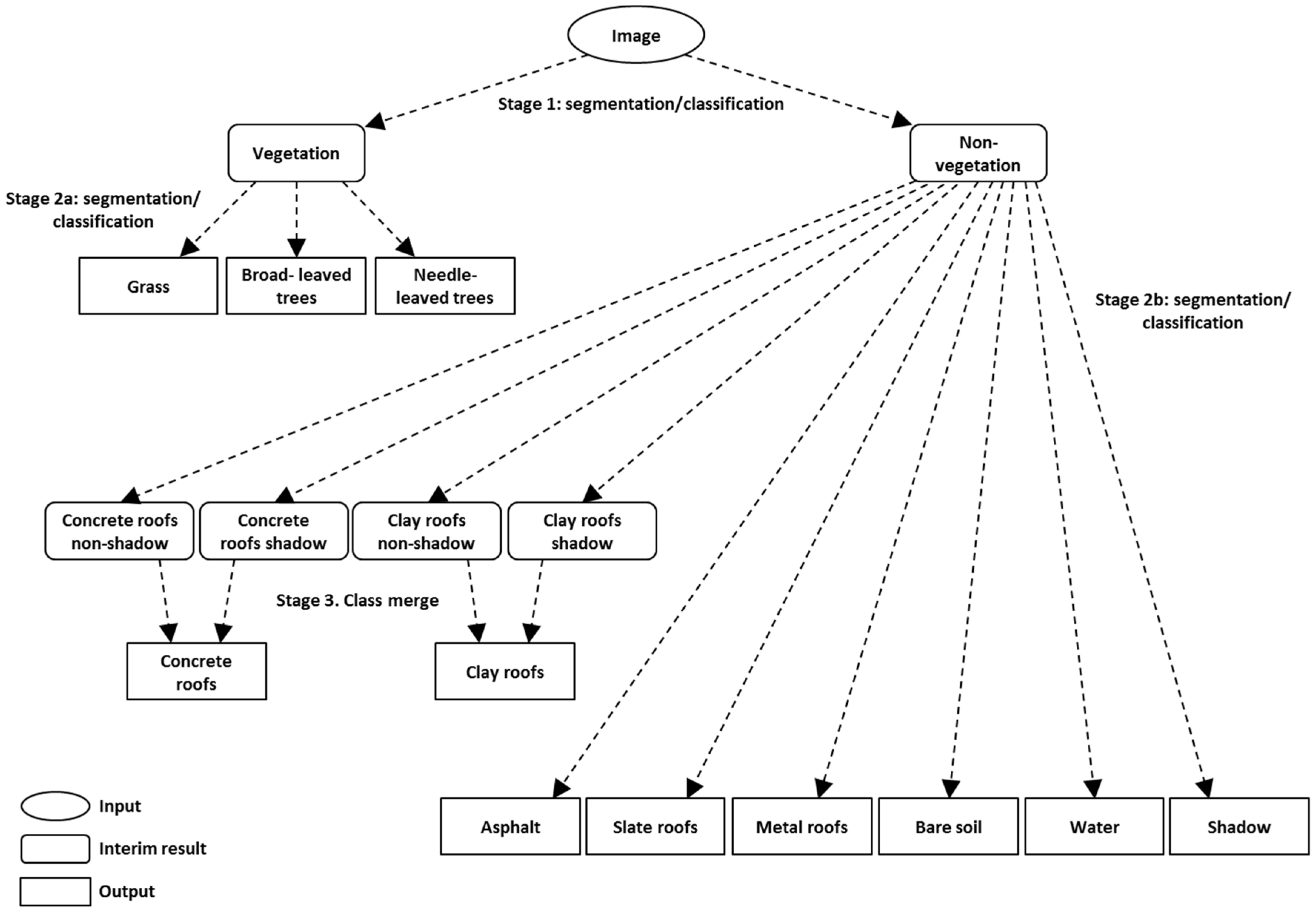
3.3. Object-Based Classification

Following pixel-based classification, object-based classification was performed on the 12 image data sets. Object-based classification operates at the scale of identifiable objects or patches in the landscape, rather than pixels. Usually these objects are derived directly from remotely sensed imagery, whereby spectrally similar neighbouring pixels are grouped together to form objects [32,51]. This is the main focus of the now established field of object-based image analysis (OBIA) or geographic object-based image analysis (GEOBIA). The development of OBIA has been linked closely with the emergence of VHR imagery since fine spatial resolution imagery is especially susceptible to within-feature (or within-object) variation and resultant pixel-based misclassification [1,19].

Object-based classification generally involves two main steps, segmentation and classification. Segmentation is conducted first, and this process can be influenced by various spatial parameters. For instance, in the case of eCognition [66] (the OBIA software package used here), the three main parameters of interest are scale, shape and compactness. These three parameters determine segmented objects on the basis of, respectively, the object’s size (determined by spatial heterogeneity), its regularity of form (i.e., the complexity of an object’s boundary configuration) and how closely packed the object’s pixels are (through comparison of the object to a circle). Following segmentation, classification is conducted on the segmented objects. Each object is classified on the basis of its pixels’ spectral information, but this can also be supplemented by additional discriminating variables such as object size and shape.

Here, considerable experimentation was conducted to determine the optimum OBIA approach, and ultimately a multi-stage (sometimes referred to as multi-scale) object-based classification procedure was developed (Figure 4). Initially, vegetation and non-vegetation features were distinguished (stage 1). Then, vegetation features were divided into their constituent classes (stage 2a), and separately non-vegetation features were divided into their constituent classes (stage 2b). Multi-stage OBIA approaches have been used widely in recent times to classify complex environments [24,67] since single-stage procedures cannot always achieve balanced segmentation outcomes for all classes of interest. That is, specific segmentation parameters may be suitable for certain classes (e.g., large areas of grassland), but lead to considerable under- (or over-) segmentation of other classes (e.g., buildings). Since multi-stage OBIA allows different parameter settings for different classes, this can achieve optimum classification outcomes for all classes [68].

Figure 4. Multi-stage object-based classification procedure.

Figure 4. Multi-stage object-based classification procedure.

A key factor for segmentation is how well segmented outputs correspond to real-world features. While the optimum shape and compactness settings remained consistent between input data sets (see Table 2 below), the scale setting had a significant impact on segmentation outcome [29]. Some recent work has promoted the use of built-in segmentation assessment, where appropriate segmentation scales are determined during the OBIA process (e.g., [69,70]). Here, we conducted sensitivity testing to compare a range of scale parameter settings and assessed their accuracy using a combination of objective metrics, as described by [71], and human assessment. 40 objects were selected randomly and compared against reference data acquired from the MasterMap vector coverage and field survey. In line with the recommendation in [72] to use multiple metrics to test the full range of segmentation characteristics, here we used five different metrics from [71] to check segmentation accuracy. The metrics employed were the Area Fit Index (AFI) which shows how closely segments overlap reference objects; two Relative Area (RA) measures, RAsub and RAsuper, which indicate over- and under-segmentation respectively; the Quality Rate (QR) which is an area-based measure that includes consideration of false positives when determining segmentation success; and the D index which is a combined metric that considers both over- and under-segmentation to indicate how closely objects produced match ideal segmentation output. See [71] for further detail on these. Collectively, the five metrics provided a strong and varied test of segmentation accuracy. Nonetheless, the somewhat arbitrary nature of accuracy metrics’ units and their sometimes conflicting outcomes [72] means that a visual check can also be useful [73,74,75]. The authors of [76] claimed that human interpretation represents the most effective means of assessing segmentation output, supported later by [77]. Therefore, ultimately, both quantitative metrics and qualitative assessment were used in combination to determine final scale settings.

Table 2. Segmentation parameter settings for multi-stage object-based classification.

Input Image Spatial Resolution (m)	Stage 1. Separation of Vegetation and Non-Vegetation		Stage 2a. Identification of Individual Vegetation Classes		Stage 2b. Identification of Individual Non-Vegetation Classes
	Segmentation Parameters (Scale, Shape, Compactness)	Spectral Merging Threshold	Segmentation Parameters (Scale, Shape, Compactness)	Spectral Merging Threshold	Segmentation Parameters (Scale, Shape, Compactness)	Spectral Merging Threshold
30	6, 0.3, 0.8	NA	7, 0.3, 0.8	NA	5, 0.3, 0.8	NA
10	10, 0.3, 0.8	NA	12, 0.3, 0.8	NA	6, 0.3, 0.8	NA
4	20, 0.3, 0.8	NA	30, 0.3, 0.8	NA	12, 0.3, 0.8	NA
2	25, 0.3, 0.8	20	35, 0.3, 0.8	35	17, 0.3, 0.8	10

Table 2. Segmentation parameter settings for multi-stage object-based classification.

Input Image Spatial Resolution (m)	Stage 1. Separation of Vegetation and Non-Vegetation		Stage 2a. Identification of Individual Vegetation Classes		Stage 2b. Identification of Individual Non-Vegetation Classes
	Segmentation Parameters (Scale, Shape, Compactness)	Spectral Merging Threshold	Segmentation Parameters (Scale, Shape, Compactness)	Spectral Merging Threshold	Segmentation Parameters (Scale, Shape, Compactness)	Spectral Merging Threshold
30	6, 0.3, 0.8	NA	7, 0.3, 0.8	NA	5, 0.3, 0.8	NA
10	10, 0.3, 0.8	NA	12, 0.3, 0.8	NA	6, 0.3, 0.8	NA
4	20, 0.3, 0.8	NA	30, 0.3, 0.8	NA	12, 0.3, 0.8	NA
2	25, 0.3, 0.8	20	35, 0.3, 0.8	35	17, 0.3, 0.8	10

Following segmentation, standard nearest neighbour classification was conducted to label objects to the most appropriate class. To ensure a fair comparison between pixel-based and object-based classification, the same training samples were used in all cases. As well as the straightforward spectral information provided by the different band sets, classification performance was enhanced (determined through trial-and-error) with additional discriminatory variables. Certain spatial object characteristics were incorporated, including area, shape and length/width ratio; and various spectral indices (described above) were also used: NDVI for all spectral band sets, plus NSDBI and NSDBRI for the 8 band set only. Finally, because of shadow effects with certain roof classes when using the 2 m spatial resolution imagery, individual buildings often tended to be classified as two objects, one representing the non-shaded side of the roof and the other representing the shaded side. Here, therefore, the concrete and clay roof classes were each first classified as two separate sub-classes (e.g., non-shadowed clay roofs, shadowed clay roofs) and then later combined to form a single (e.g., clay roofs) class (Figure 4, stage 3).

In the past, considerable attention has focused on specific OBIA parameter settings, especially for the widely used eCognition [29], though this has created some difficulties for transferability since the OBIA process can be highly idiosyncratic to each particular study or image data set. As such, there is only limited benefit in reporting parameter settings, since these may not be directly transferable to another context. However, here, for completeness, but especially since this study is principally concerned with comparison between spatial, spectral and classifier characteristics using a common study area and data set, parameter settings are presented in Table 2. Notably, it is interesting to compare settings between the different spatial resolution inputs (30 m, 10 m, 4 m, 2 m), bearing in mind that in each case sensitivity testing was used to optimize classification outcome. It can be seen that the shape and compactness settings are consistent throughout all 12 classifications, whereas the optimum scale setting increased consistently from 30 m to 2 m resolution. Broadly speaking, increasing the scale parameter increases average segment size, and this makes sense in the current context whereby the higher scale settings at finer resolutions offset smaller pixel sizes, leading to consistently sized objects (i.e., consistent between varying input spatial resolution). Also, the optimum scale setting was consistently larger for vegetation classes (e.g., large parcels of grassland and woodland) than non-vegetation classes (e.g., small urban features such as buildings and roads). Finally, following segmentation, a merging procedure can be used to combine spectrally similar objects thus refining the final segmented output. Here, this proved helpful only in the case of the input 2 m spatial resolution data, since the complexity of this imagery led inevitably to some degree of over-segmentation.

3.4. Accuracy Assessment and Statistical Testing

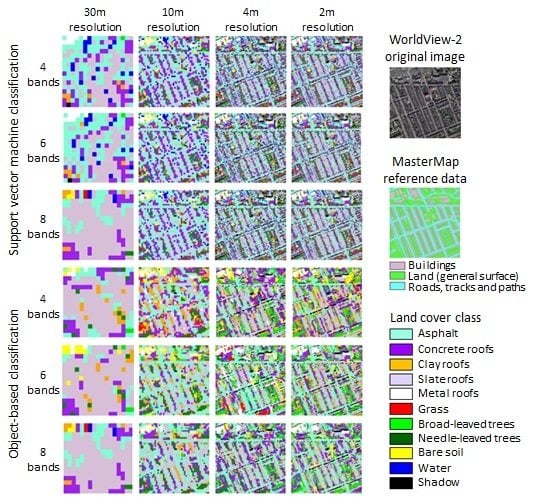
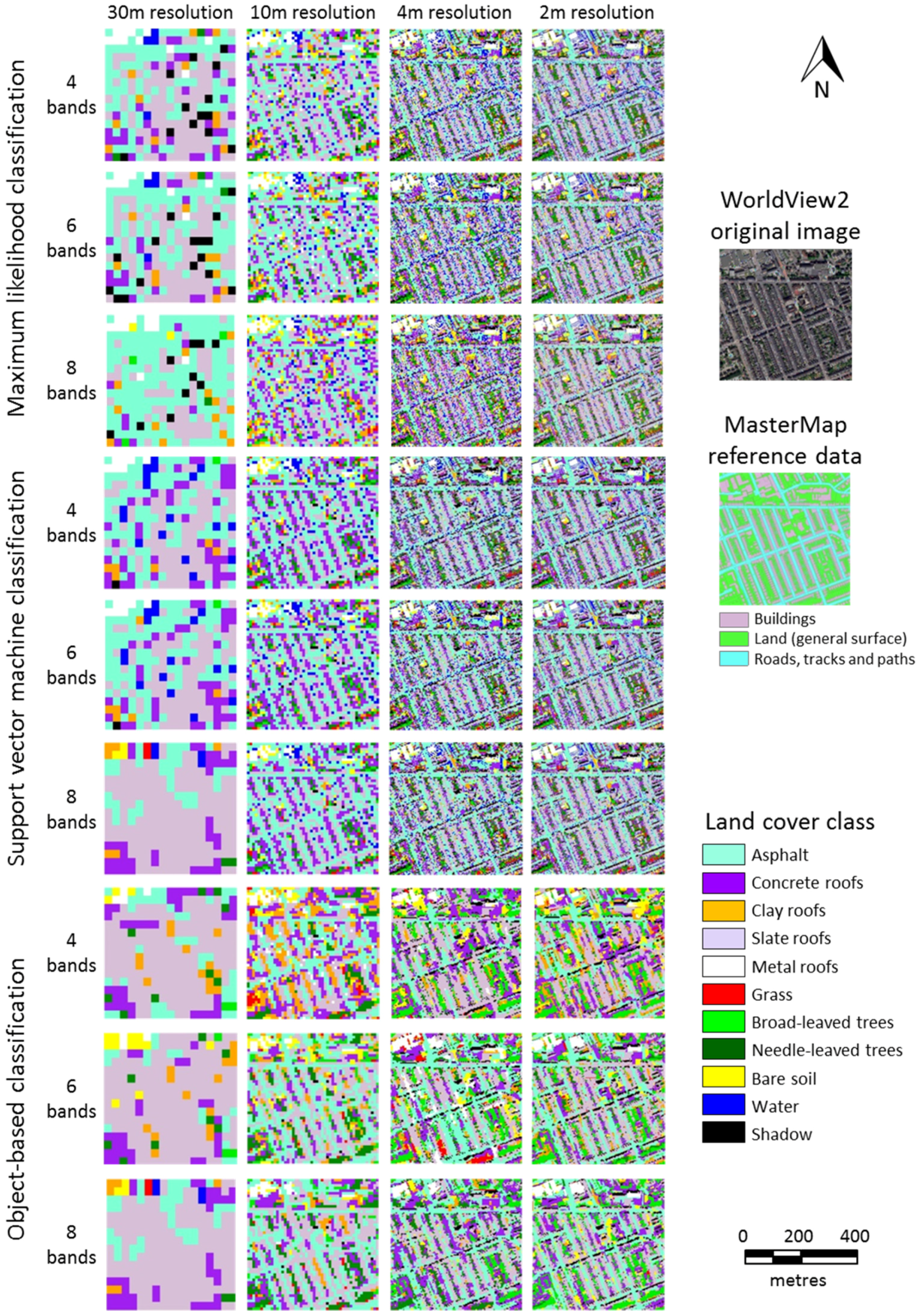
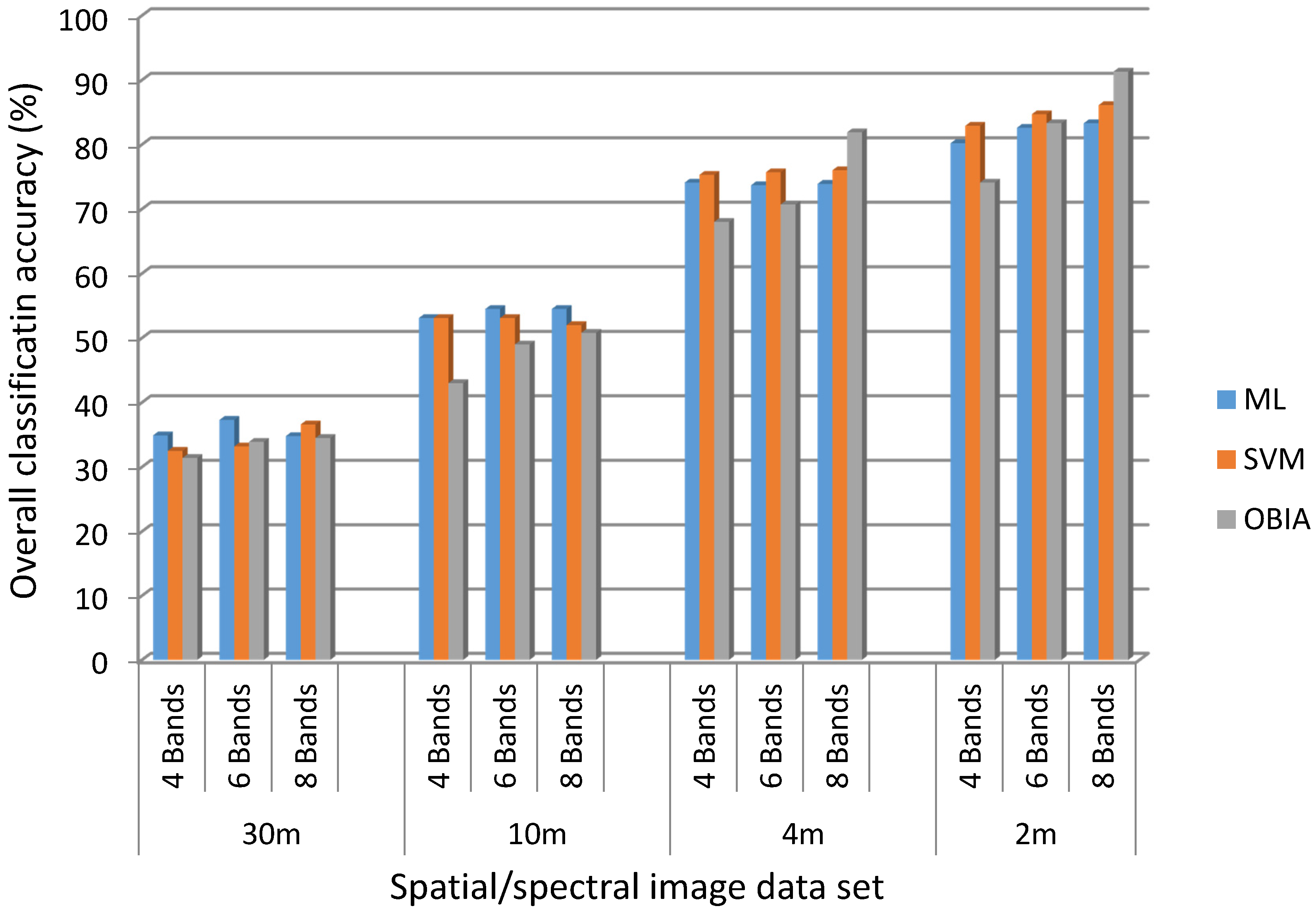
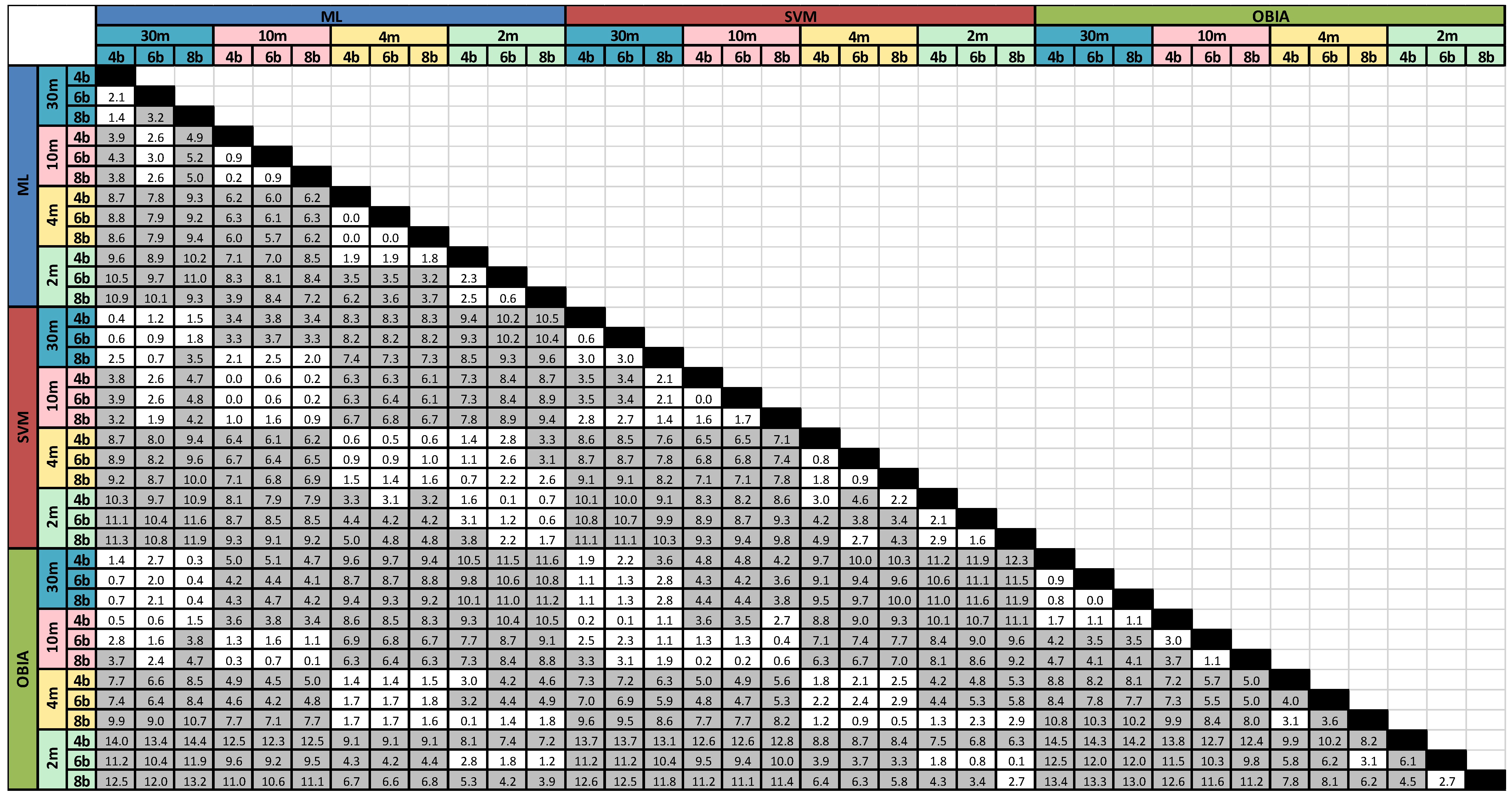
Following classification, the 36 output land cover maps were tested against reference data to calculate their accuracy. To enable direct comparison between the three different classification approaches, it was necessary to adopt a common means of accuracy assessment, so point-based checking was conducted. It is important to note that alternative object-based approaches are now available for use with OBIA outputs [78,79,80,81], and these can have the benefit of providing an exact match between analysis data (i.e., classified objects) and reference data (e.g., vector map features). In total, 438 sample points were checked, with between 30 and 43 points used for each individual class. The same points were used for all classification outputs, ensuring direct comparability between results. Confusion or error matrices were generated to show correspondence between predicted (classified) and reference class labels, indicating class-level accuracies (including users and producers accuracy), inter-class confusion or error, and overall classification accuracy.

While error matrices provide a useful means of comparing classification results, they can only provide an “estimate” of classification accuracy (based on the sample of points used), and therefore only tentative conclusions can be drawn [82]. This is especially the case where differences in accuracy are marginal, for instance a few percentage points apart. For example, it may be unwise to assert that a land cover map with an accuracy of, say, 93% is definitively more accurate than a map with 89% accuracy. This 4% difference may in fact be a statistical artefact of the sample of test points. The authors of [83] state that accuracy statements should be compared in a statistically rigorous manner and the results expressed with confidence limits. Here, the McNemar test was used to compare classification outputs and indicate the statistical significance of any difference in results [82]. That is, in the example above, the McNemar test could indicate whether or not a difference of 4% is statistically significant. As [82] notes this is a non-parametric test that is focused on the binary distinction between correct and incorrect class allocations of two classification outputs (LC map 1 and LC map 2). The McNemar test calculates the z value:

$$\text{z} = \frac{f_{1 2}- f_{21}}{\sqrt{f_{1 2}+ f_{21}}}$$

(1)

where f₁₂ indicates the total number of paired class allocations correct in LC map 1 but incorrect in LC map 2, and f₂₁ indicates the total number of paired class allocations correct in LC map 2 but incorrect in LC map 1. If z ≥ 3.2, this demonstrates a significant difference between two LC maps at the 99% confidence level [84]. Here, a fully rigorous and exhaustive approach was adopted for expressing the statistical significance of classification output differences. The McNemar test was conducted on every possible pair of classified land cover maps. With 36 original maps, this meant 630 paired combinations. The results, expressed as a matrix, enable straightforward comparison between all classifications, clearly identifying those classification pairs that are significantly different and those that are not.

4. Results

In total, 36 land cover maps were produced, using a combination of four spatial resolutions (30 m, 10 m, 4 m, 2 m), three spectral band sets (4 bands, 6 bands, 8 bands) and three classifiers (ML, SVM, OBIA). The main aim of this paper is to provide a comprehensive comparison between these variables, so for completeness extracts of all 36 classified maps are provided in Figure 5. Note, this figure should be interpeted with some caution since it shows only one small area and is not therefore fully representative of land cover throughout the whole study extent. Nonetheless, the figure clearly shows the most significant and consistent pattern evident throughout the results: classification improves as spatial resolution becomes finer.

Figure 5. Land cover maps (detail) for the 36 data set/classifier combinations, plus the WorldView-2 image (© DigitalGlobe, Inc. All Rights Reserved) and MasterMap vector data (© Crown Copyright and Database Right 2015. Ordnance Survey (Digimap Licence).

Figure 5. Land cover maps (detail) for the 36 data set/classifier combinations, plus the WorldView-2 image (© DigitalGlobe, Inc. All Rights Reserved) and MasterMap vector data (© Crown Copyright and Database Right 2015. Ordnance Survey (Digimap Licence).

While the full set of statistical classification results are summarized below, two full error matrices are first presented to give some examples of class-level detail. To provide contrast and show the full range of classification success, the most accurate classification overall (2 m, 8 bands, OBIA) and least accurate classification overall (30 m, 4 bands, OBIA) are presented (Table 3 and Table 4, respectively). The highest overall classification accuracy (91%) was achieved by arguably the most sophisticated data set/classifier combination, using the most advanced spatial and spectral characteristics of WV2 imagery and state-of-the-art OBIA (Table 3). This classification enabled relatively accurate mapping of all classes, with only minor confusion between vegetation classes and between concrete and other impervious classes. In contrast, it is clear that the less sophisticated data set/classifier combination (using relatively coarse 30 m resolution and only four basic spectral bands) is wholly inadequate in classifying such detailed urban land cover classes (Table 4). Few classes are mapped with any success and overall classification accuracy is only 35%. Perhaps the most significant factor here, as will be discussed below, is the coarse spatial resolution, which prevents accurate identification of small urban features.

A summary of classification accuracies for all 36 land cover maps is provided in Figure 6. This figure presents raw overall classification accuracies and enables direct assessment of the differences between classifications. However, this does not indicate which of these differences are statistically significant. Therefore, a full matrix of z values (calculated from the McNemar test of statistical significance) between all 630 classification pairs is also presented, in Figure 7. Statistically significant differences (i.e., z values ≥ 3.2, at the 99% confidence level) are highlighted in grey. Note, the figure clearly contains a large volume of information and requires careful interpretation, but it is included here to enable comprehensive and unlimited comparison between data set/classifier combinations.

Figure 6. Overall land cover classification accuracies for the 36 data set/classifier combinations (ML = maximum likelihood, SVM = support vector machine, OBIA = object-based image analysis).

Figure 6. Overall land cover classification accuracies for the 36 data set/classifier combinations (ML = maximum likelihood, SVM = support vector machine, OBIA = object-based image analysis).

Table 3. Error matrix for the OBIA classification using 2 m spatial resolution, 8 spectral band imagery.

		Reference Class											Users Accuracy
		Asphalt	Concrete Roofs	Clay Roofs	Metal Roofs	Slate Roofs	Grass	Broad-leaved Trees	Needle-leaved trees	Bare Soil	Water	Shadow
Predicted Class	Asphalt	37	1	1	0	1	0	0	0	0	0	0	93%
	Concrete roofs	4	38	4	0	3	0	0	0	0	0	0	78%
	Clay roofs	0	1	34	0	1	0	0	0	0	0	0	94%
	Metal roofs	0	0	0	39	0	0	0	0	0	0	0	100%
	Slate roofs	1	1	0	0	35	0	0	0	0	0	0	95%
	Grass	1	0	0	0	0	36	0	0	1	0	1	92%
	Broad-leaved trees	0	0	0	0	0	5	40	8	0	0	0	75%
	Needle-leaved trees	0	0	0	0	0	0	2	30	0	0	0	94%
	Bare soil	0	0	1	1	0	0	0	0	29	0	0	94%
	Water	0	0	0	0	0	0	0	0	0	43	0	100%
	Shadows	0	0	0	0	0	0	0	0	0	0	39	100%
Producers accuracy		86%	93%	85%	98%	88%	88%	95%	79%	97%	100%	98%
Overall classification accuracy = 91%

Table 3. Error matrix for the OBIA classification using 2 m spatial resolution, 8 spectral band imagery.

		Reference Class											Users Accuracy
		Asphalt	Concrete Roofs	Clay Roofs	Metal Roofs	Slate Roofs	Grass	Broad-leaved Trees	Needle-leaved trees	Bare Soil	Water	Shadow
Predicted Class	Asphalt	37	1	1	0	1	0	0	0	0	0	0	93%
	Concrete roofs	4	38	4	0	3	0	0	0	0	0	0	78%
	Clay roofs	0	1	34	0	1	0	0	0	0	0	0	94%
	Metal roofs	0	0	0	39	0	0	0	0	0	0	0	100%
	Slate roofs	1	1	0	0	35	0	0	0	0	0	0	95%
	Grass	1	0	0	0	0	36	0	0	1	0	1	92%
	Broad-leaved trees	0	0	0	0	0	5	40	8	0	0	0	75%
	Needle-leaved trees	0	0	0	0	0	0	2	30	0	0	0	94%
	Bare soil	0	0	1	1	0	0	0	0	29	0	0	94%
	Water	0	0	0	0	0	0	0	0	0	43	0	100%
	Shadows	0	0	0	0	0	0	0	0	0	0	39	100%
Producers accuracy		86%	93%	85%	98%	88%	88%	95%	79%	97%	100%	98%
Overall classification accuracy = 91%

Table 4. Error matrix for the OBIA classification using 30 m spatial resolution, 4 spectral band imagery.

		Reference Class											Users Accuracy
		Asphalt	Concrete Roofs	Clay Roofs	Metal Roofs	Slate Roofs	Grass	Broad-leaved Trees	Needle-leaved Trees	Bare Soil	Water	Shadow
Predicted Class	Asphalt	14	9	2	5	7	2	7	0	3	6	12	23%
	Concrete roofs	16	18	15	1	11	0	4	1	2	3	7	33%
	Clay roofs	6	6	18	2	6	5	4	3	0	0	5	71%
	Metal roofs	0	0	0	25	2	0	0	0	2	0	6	57%
	Slate roofs	3	3	1	0	12	0	0	0	0	0	2	44%
	Grass	0	1	0	0	0	12	7	5	2	0	0	26%
	Broad-leaved trees	0	2	1	0	1	12	13	16	3	1	1	15%
	Needle-leaved trees	0	0	0	0	0	1	4	2	0	5	1	32%
	Bare soil	3	3	1	7	0	6	1	9	16	2	2	76%
	Water	0	1	0	0	0	2	0	0	0	22	4	0%
	Shadows	0	0	2	0	2	0	2	1	2	3	0	23%
Producers accuracy		33%	42%	45%	63%	29%	30%	31%	5%	53%	52%	0%
Overall classification accuracy = 35%

Table 4. Error matrix for the OBIA classification using 30 m spatial resolution, 4 spectral band imagery.

		Reference Class											Users Accuracy
		Asphalt	Concrete Roofs	Clay Roofs	Metal Roofs	Slate Roofs	Grass	Broad-leaved Trees	Needle-leaved Trees	Bare Soil	Water	Shadow
Predicted Class	Asphalt	14	9	2	5	7	2	7	0	3	6	12	23%
	Concrete roofs	16	18	15	1	11	0	4	1	2	3	7	33%
	Clay roofs	6	6	18	2	6	5	4	3	0	0	5	71%
	Metal roofs	0	0	0	25	2	0	0	0	2	0	6	57%
	Slate roofs	3	3	1	0	12	0	0	0	0	0	2	44%
	Grass	0	1	0	0	0	12	7	5	2	0	0	26%
	Broad-leaved trees	0	2	1	0	1	12	13	16	3	1	1	15%
	Needle-leaved trees	0	0	0	0	0	1	4	2	0	5	1	32%
	Bare soil	3	3	1	7	0	6	1	9	16	2	2	76%
	Water	0	1	0	0	0	2	0	0	0	22	4	0%
	Shadows	0	0	2	0	2	0	2	1	2	3	0	23%
Producers accuracy		33%	42%	45%	63%	29%	30%	31%	5%	53%	52%	0%
Overall classification accuracy = 35%

The most obvious finding is the clear correlation between spatial resolution and classification accuracy. As spatial resolution becomes finer—from 30 m, through 10 m and 4 m, to 2 m—classification accuracy increases consistently, with all spectral band sets and all classifiers (Figure 6). Moreover, these differences across resolutions (i.e., comparing common spectral band sets and classifiers) are all statistically significant (Figure 7). At the coarsest resolution (30 m), accuracy ranges between 30% and 40%; while the finest (2 m) resolution imagery leads to accuracies routinely in the 80s%, and at maximum in excess of 90% (Table 3). This finding reaffirms the contention that accurate and detailed mapping of complex urban environments requires spatially detailed data, and here contemporary VHR imagery holds considerable value for the mapping community.

The relationship between the number of spectral bands and classification accuracy is less marked than that of spatial resolution. Nonetheless, overall, increasing the number of spectral bands—from 4, through 6, to 8—does lead to modest increases in classification accuracy (Figure 6), though these are not always statistically significant (Figure 7). This trend is consistent at all spatial resolutions, though more pronounced at the finer (4 m and especially 2 m) resolutions than the coarser (30 m and 10 m) resolutions. For instance, for the 2 m resolution imagery, average accuracy (i.e., the average of all three classifiers) increases from 79.1% when using 4 bands, to 83.5% when using 6 bands and 86.9% when using 8 bands. In contrast, for the 30 m imagery, average accuracy increases only very slightly from 32.9% for 4 bands, to 34.8% for 6 bands and 35.3% for 8 bands. (Note, the influence of the number of spectral bands on classification accuracy also depends on the classifier used, as discussed below.) This finding demonstrates that enhanced spectral information can aid distinction of detailed thematic classes in complex environments. Notably, here, the additional bands offered by contemporary VHR sensors such as WV2 and WV3 may offer some advantage over early VHR sensors such as IKONOS.

The influence of choice of classifier on classification accuracy is more complex than that of spatial resolution or spectral band set. The results show that the classifier can have a noticable effect on accuracy, but only when considered in combination with spatial resolution and/or number of spectral bands (Figure 6). At the coarsest spatial resolution (30 m), differences between classifiers are marginal, and generally not statistically significant (Figure 7). However, it is interesting to note that the ML classifier performs slightly better overall at this resolution (or at least no worse, when factoring in statistical significance) than the more sophisticated SVM and OBIA approaches. This pattern continues at the next finest resolution (10 m), and here both pixel-based classifiers (ML, SVM) also prove significantly more accurate than OBIA.

At the finest spatial resolutions (4 m, 2 m), patterns related to choice of classifier change from those observed at the coarser resolutions, and also become more defined (Figure 6). The SVM classifier is now consistently (often significantly) more accurate than the ML classifer (Figure 7). For instance, for the 4 m resolution imagery, average SVM accuracy (i.e., the average of all three spectral band sets) is 75.7%, compared to an average ML accuracy of 73.9%. At 2 m resolution, the difference is even more pronounced: average SVM accuracy = 84.6%, average ML accuracy = 82%.

The most distinct classifier/accuracy pattern, though, relates to OBIA accuracy and how this increases as both spatial resolution becomes finer and the number of spectral bands increases. At the smallest band set (four spectral bands), OBIA is consistently the least accurate of the three classifiers. For instance, at 2 m resolution, 4 band OBIA accuracy is 74.1%, considerably lower than 4 band ML (80.2%) and SVM (82.9%) accuracy. However, at the largest band set (eight spectral bands), this relationship is reversed and OBIA is significantly more accurate (91.3%) than SVM (86.1%) or ML (83.3%). These findings demonstrate that the choice of classifier can influence the accuracy with which complex urban environments are mapped, but due consideration should also be given to image characteristics. Contemporary classification approaches such as pixel-based SVM and OBIA perhaps hold considerable potential here where state-of-the-art VHR imagery (i.e., with enhanced spectral capabilities) are available.

Figure 7. Matrix of McNemar test z values showing the statistical significance of differences between all classification pairs (ML = maximum likelihood, SVM = support vector machine, OBIA = object-based image analysis; 30 m, 10 m, 4 m and 2 m refer to spatial resolution; 4b, 6b and 8b refer to the number of spectral bands; z values ≥ 3.2 (highlighted grey) are statistically significant at the 99% confidence level).

Figure 7. Matrix of McNemar test z values showing the statistical significance of differences between all classification pairs (ML = maximum likelihood, SVM = support vector machine, OBIA = object-based image analysis; 30 m, 10 m, 4 m and 2 m refer to spatial resolution; 4b, 6b and 8b refer to the number of spectral bands; z values ≥ 3.2 (highlighted grey) are statistically significant at the 99% confidence level).

5. Discussion

5.1. The Key Role of Spatial Resolution

Spatial resolution is the most significant factor in determining the success or otherwise of mapping complex urban land cover (Figure 6); this is clear, and indeed unsurprising [21]. VHR satellite sensor imagery has proved a game-changer here, obviously increasing the spatial detail and spatial accuracy of urban land cover maps as compared against medium resolution imagery, but also substantially increasing the level of thematic detail. While Landsat-like image classifications were often limited to a single general “urban” class [11,85], VHR imagery enables many constituent urban land cover types to be discriminated [35,86].

5.2. Spectral Data Dimensionality

While the role of spatial resolution in urban mapping is fairly straightforward, the role of image spectral characteristics is less clear. Recent VHR sensors such as WV2 and WV3 now have enhanced spectral capabilities compared to early generation VHR instruments like IKONOS and QuickBird. It should be noted the new bands provided by WV2 and WV3—coastal, yellow, red edge and NIR2—were not necessarily developed with urban environments in mind. Instead, the main stated intentions were to enhance capabilities for bathymetry (coastal) and vegetation (yellow, red edge, NIR2) analysis. However, we show some evidence here that the greater spectral capability of WV2 can indeed increase urban mapping accuracy over old four-band, e.g., IKONOS, imagery (Figure 6). This benefit is most pronounced, and only really statistically significant, at the finest spatial resolutions, and especially using OBIA.

When designing this experiment, we did wonder whether the Hughes effect would play any obvious role in influencing classification accuracy. This effect refers to the “curse of dimensionality” where adding spectral bands can in fact reduce classification accuracy, essentially since more statistical demands are being made of (inherently limited or sparse) training data. Clearly, any such effect would counteract the intuitive expectation, as here, that added spectral detail should increase class separation. Overall, there was no noticable Hughes effect. Generally classification accuracy stayed static or increased modestly as the number of spectral bands increased; there were certainly no obvious cases where accuracy decreased (Figure 6). This outcome seems satisactory. The Hughes effect is perhaps more of a concern with higher dimension, e.g., hyperspectral, data, where it may be necessary to perform data reduction on a data set with 10s or 100s of spectral bands [87]. It seems WV2’s eight-band data set is sufficiently small not to invoke any Hughes effect. This is useful since it means there would be no particular need to consider data reduction at the outset of any project, at least from an accuracy perspective (there may be other, e.g., computer processing time, considerations).

5.3. Classifier Choice

Choice of classifier is important in determining the success of classifying complex urban environments and the optimum choice will vary depending on image data characterstics. First, we consider the comparison between parametric (ML) and non-parametric (SVM) pixel-based approaches. An interesting pattern emerged here: ML was generally more accurate at the coarser spatial resolutions, but this trend was reversed at the finer resolutions with SVM becoming superior (Figure 6). This outcome is likely explained by the quality of the training data at the different resolutions and the fact that SVMs are better able than ML to handle complex, noisy data (i.e., as may occur at finer resolutions) [18]. As might be expected, this finding was most pronounced at the finest, 2 m, resolution, where differences between SVM and ML were generally statistically significant (Figure 7).

Next, we consider the comparison between pixel- and object-based approaches. Here, somewhat surprisingly, at the coarser spatial resolutions, pixel-based approaches tended to be more accurate than OBIA (Figure 6). In fact, even at the finer resolutions, for small spectral band sets (4 bands, and sometimes even 6 bands), ML and SVM outperformed OBIA. However, for the most sophisticated and complex data sets (2 m/8 bands; also 4 m/8 bands), OBIA was markedly (and significantly, Figure 7) more accurate. Indeed the OBIA classification of the 2 m resolution, 8 band data set was comfortably the most accurate result overall (Table 3). This finding reinforces the contention that OBIA is particularly well suited for VHR imagery [88,89,90]. At this fine scale of observation, within-feature variation is likely which may well lead to pixel-based misclassification, but may be mitigated by aggregation at the scale of the object. It is interesting, though, that the number of spectral bands has a noticable influence on OBIA classification accuracy, and the results imply that contemporary VHR instruments with enhanced spectral capabilities have particular potential for urban mapping, holding a considerable advantage over early VHR sensors.

When considering pixel- and object-based classification accuracy, it should be noted that a point-based assessment procedure was adopted since this enabled direct comparison between the different classification approaches. However, some practitioners have recently promoted the uptake of object-based assessment procedures, suggesting they may provide a more appropriate test of OBIA outputs [78,79,80,81].

5.4. Project Requirements versus Project Resources

This research presents various data and analysis considerations for urban mapping projects. The other essential consideration relates to project resourcing, since this will have a bearing on both the imagery acquired and the methodology employed. The results here show that VHR imagery is essential for accurate, detailed thematic mapping of urban land cover. Unfortunately this imagery can be costly, unlike the free provision of all Landsat data. Moreover, the more advanced image products (e.g., 2 m, 8 band WV3 imagery) tend to be considerably more expensive than basic (e.g., 4 m, 2 band) products. Also important here are computer, software and operator resources, and in general OBIA approaches tend to require more resource than pixel-based classification approaches. For instance, OBIA generally involves considerably more operator input than ML or SVM analysis, some OBIA operations require substantial computer processing resources, and OBIA packages can be relatively costly. This experiment found OBIA classification of 2 m spatial resolution, 8 spectral band imagery most accurate, though this combination is perhaps the most expensive in terms of resourcing. Satisfactory, cheaper alternatives may exist, depending on user requirements. Here, for instance, SVM classification of 2 m, 4 band data resulted in only a fairly modest decrease in accuracy against the maximum, and this approach would incur considerable savings in terms of data costs (4 band WV2 or WV3 imagery), software requirements (no OBIA purchase) and manpower (reduced operator time).

6. Conclusions

This paper presents an exhaustive practical experiment to demonstrate the success of contemporary spaceborne imagery and classification methodologies for mapping complex urban environments. This is a unique investigation to provide a full test of the latest VHR imagery for detailed urban classification, examining the influence of spatial resolution and spectral band set, as well as comparing traditional and modern classification approaches. In contrast, previous studies have generally tended to conduct limited comparisons between, for instance, coarse and fine resolution or pixel- and object-based classification. A detailed, 11 class classification schema is used here to identify the maximum level of thematic information that can be achieved using VHR imagery. Again, this contrasts with earlier work that has usually opted for few, broad land cover classes. Finally, our work is conducted on a relatively large image area, the city of Nottingham, UK and its environs, ensuring that urban land cover information is generated at a scale of practical value. In contrast, earlier experiments have often been limited to very small, local areas.

Overall, it is clear that spatial resolution is the most influential factor in enabling accurate mapping of complex urban environments: the finer the resolution, the higher the accuracy. New VHR sensors offer huge potential here, and ongoing technological advancement (and accompanying changes in legislation) implies that opportunities will continue to grow. WV3 was launched in 2014 with the potential for acquiring multispectral (8 band) imagery at a resolution of 1.2 m. Crucially, in 2015 new U.S. governmental legislation was passed that then allowed this image resolution to be made available to commercial users. While not as influential as spatial resolution, the new spectral capabilities provided by, for instance, WV3 can also lead to modest increases in urban mapping accuracy. This advantage is maximized through the use of contemporary, e.g., SVM and especially OBIA, classification approaches, when compared against traditional ML classification. Overall, state-of-the-art VHR imagery (2 m resolution, 8 bands) and OBIA classification provides the most accurate combination for mapping complex urban land cover, but this is perhaps also the most costly and resource-hungry approach. Where resources are limited, requiring some compromise between imagery and methodology, the recommended order of priority is, first, spatial resolution (as fine as possible); second, classifier (first choice OBIA, second choice SVM); and, third, spectral band set (8 bands if possible).

References

1. Lu, D.; Weng, Q. A survey of image classification methods and techniques for improving classification performance. Int. J. Remote Sens. 2007, 28, 823–870. [Google Scholar] [CrossRef]
2. Zhou, Y.H.; Qiu, F. Fusion of high spatial resolution WorldView-2 imagery and LIDAR pseudo-waveform for object-based image analysis. ISPRS J. Photogramm. Remote Sens. 2015, 101, 221–232. [Google Scholar] [CrossRef]
3. Xu, H.Q. Rule-based impervious surface mapping using high spatial resolution imagery. Int. J. Remote Sens. 2013, 34, 27–44. [Google Scholar] [CrossRef]
4. Herold, M.; Gardner, M.E.; Roberts, D.A. Spectral resolution requirements for mapping urban areas. IEEE Trans. Geosci. Remote Sens. 2003, 41, 1907–1919. [Google Scholar] [CrossRef]
5. Lu, D.S.; Hetrick, S.; Moran, E. Land cover classification in a complex urban-rural landscape with QuickBird imagery. Photogramm. Eng. Remote Sens. 2010, 76, 1159–1168. [Google Scholar] [CrossRef]
6. Moreira, R.C.; Galvão, L.S. Variation in spectral shape of urban materials. Remote Sens. Lett. 2010, 1, 149–158. [Google Scholar] [CrossRef]
7. Guindon, B.; Zhang, Y.; Dillabaugh, C. Landsat urban mapping based on a combined spectral-spatial methodology. Remote Sens. Environ. 2004, 92, 218–232. [Google Scholar] [CrossRef]
8. Small, C.; Lu, J.W.T. Estimation and vicarious validation of urban vegetation abundance by spectral mixture analysis. Remote Sens. Environ. 2006, 100, 441–456. [Google Scholar] [CrossRef]
9. Lu, D.S.; Hetrick, S.; Moran, E. Impervious surface mapping with QuickBird imagery. Int. J. Remote Sens. 2011, 32, 2519–2533. [Google Scholar] [CrossRef] [PubMed]
10. Ling, F.; Li, X.; Xiao, F.; Fang, S.; Du, Y. Object-based sub-pixel mapping of buildings incorporating the prior shape information from remotely sensed imagery. Int. J. Appl. Earth Obs. Geoinform. 2012, 18, 283–292. [Google Scholar] [CrossRef]
11. Zhang, J.; Li, P.; Wang, J. Urban built-up area extraction from Landsat TM/ETM+ images using spectral information and multivariate texture. Remote Sens. 2014, 6, 7339–7359. [Google Scholar] [CrossRef]
12. Aplin, P. Remote sensing: Base mapping. Prog. Phys. Geogr. 2003, 27, 275–283. [Google Scholar] [CrossRef]
13. Inglada, J.; Michel, J. Qualitative spatial reasoning for high-resolution remote sensing image analysis. IEEE Trans. Geosci. Remote Sens. 2009, 47, 599–612. [Google Scholar] [CrossRef] [Green Version]
14. Weng, Q. Remote sensing of impervious surfaces in the urban areas: Requirements, methods, and trends. Remote Sens. Environ. 2012, 117, 34–49. [Google Scholar] [CrossRef]
15. Qin, Y.C.; Li, S.H.; Vu, T.T.; Niu, Z.; Ban, Y.F. Synergistic application of geometric and radiometric features of LIDAR data for urban land cover mapping. Opt. Express 2015, 23, 13761–13775. [Google Scholar] [CrossRef] [PubMed]
16. Tuia, D.; Pacifici, F.; Kanevski, M.; Emery, W.J. Classification of very high spatial resolution imagery using mathematical morphology and support vector machines. IEEE Trans. Geosci. Remote Sens. 2009, 47, 3866–3879. [Google Scholar] [CrossRef]
17. Fiumi, L. Surveying the roofs of Rome. J. Cult. Herit. 2012, 13, 304–313. [Google Scholar] [CrossRef]
18. Poursanidis, D.; Chrysoulakis, N.; Mitraka, Z. Landsat 8 vs. Landsat 5: A comparison based on urban and peri-urban land cover mapping. Int. J. Appl. Earth Obs. Geoinform. 2015, 35, 259–269. [Google Scholar] [CrossRef]
19. Blaschke, T.; Hay, G.J.; Kelly, M.; Lang, S.; Hofmann, P.; Addink, E.; Feitosa, R.Q.; van der Meer, F.; van der Werff, H.; van Coillie, F.; et al. Geographic object-based image analysis—Towards a new paradigm. ISPRS J. Photogramm. Remote Sens. 2014, 87, 180–191. [Google Scholar] [CrossRef] [PubMed]
20. Lu, D.S.; Weng, Q.H. Spectral mixture analysis of the urban landscape in Indianapolis with Landsat ETM plus imagery. Photogramm. Eng. Remote Sens. 2004, 70, 1053–1062. [Google Scholar] [CrossRef]
21. Myint, S.W.; Gober, P.; Brazel, A.; Grossman-Clarke, S.; Weng, Q.H. Per-pixel vs. object-based classification of urban land cover extraction using high spatial resolution imagery. Remote Sens. Environ. 2011, 115, 1145–1161. [Google Scholar] [CrossRef]
22. Campbell, J.B. Introduction to Remote Sensing, 4th ed.; Guilford Press: New York, NY, USA, 2007. [Google Scholar]
23. Aplin, P.; Smith, G.M. Introduction to object-based landscape analysis. Int. J. Geogr. Inf. Sci. 2011, 25, 869–875. [Google Scholar] [CrossRef]
24. Liu, J.J.; Shi, L.S.; Zhang, C.; Yang, J.Y.; Zhu, D.H.; Yang, J.H. A variable multi-scale segmentation method for spatial pattern analysis using multispectral WorldView-2 images. Sensor Lett. 2013, 11, 1055–1061. [Google Scholar] [CrossRef]
25. Huang, X.; Zhang, L.P. An SVM ensemble approach combining spectral, structural, and semantic features for the classification of high-resolution remotely sensed imagery. IEEE Trans. Geosci. Remote Sens. 2013, 51, 257–272. [Google Scholar] [CrossRef]
26. Mountrakis, G.; Im, J.; Ogole, C. Support vector machines in remote sensing: A review. ISPRS J. Photogramm. Remote Sens. 2011, 66, 247–259. [Google Scholar] [CrossRef]
27. Myint, S.W.; Mesev, V. A comparative analysis of spatial indices and wavelet-based classification. Remote Sens. Lett. 2012, 3, 141–150. [Google Scholar] [CrossRef]
28. Zhou, W.Q.; Troy, A.; Grove, M. Object-based land cover classification and change analysis in the Baltimore metropolitan area using multitemporal high resolution remote sensing data. Sensors 2008, 8, 1613–1636. [Google Scholar] [CrossRef]
29. Li, X.X.; Shao, G.F. Object-based land-cover mapping with high resolution aerial photography at a county scale in midwestern USA. Remote Sens. 2014, 6, 11372–11390. [Google Scholar] [CrossRef]
30. Walker, J.S.; Blaschke, T. Object-based land-cover classification for the Phoenix metropolitan area: Optimization vs. transportability. Int. J. Remote Sens. 2008, 29, 2021–2040. [Google Scholar] [CrossRef]
31. Bhaskaran, S.; Paramananda, S.; Ramnarayan, M. Per-pixel and object-oriented classification methods for mapping urban features using IKONOS satellite data. Appl. Geogr. 2010, 30, 650–665. [Google Scholar] [CrossRef]
32. Blaschke, T.; Hay, G.J.; Weng, Q.; Resch, B. Collective sensing: Integrating geospatial technologies to understand urban systems—An overview. Remote Sens. 2011, 3, 1743–1776. [Google Scholar] [CrossRef]
33. Baker, B.A.; Warner, T.A.; Conley, J.F.; McNeil, B.E. Does spatial resolution matter? A multi-scale comparison of object-based and pixel-based methods for detecting change associated with gas well drilling operations. Int. J. Remote Sens. 2013, 34, 1633–1651. [Google Scholar] [CrossRef]
34. Jebur, M.N.; Shafri, H.Z.M.; Pradhan, B.; Tehrany, M.S. Per-pixel and object-oriented classification methods for mapping urban land cover extraction using SPOT 5 imagery. Geocarto Int. 2014, 29, 792–806. [Google Scholar] [CrossRef]
35. Bouziani, M.; Goita, K.; He, D.C. Rule-based classification of a very high resolution image in an urban environment using multispectral segmentation guided by cartographic data. IEEE Trans. Geosci. Remote Sens. 2010, 48, 3198–3211. [Google Scholar] [CrossRef]
36. Ziaei, Z.; Pradhan, B.; Bin Mansor, S. A rule-based parameter aided with object-based classification approach for extraction of building and roads from WorldView-2 images. Geocarto Int. 2014, 29, 554–569. [Google Scholar] [CrossRef]
37. Hamedianfar, A.; Shafri, H.Z.M.; Mansor, S.; Ahmad, N. Improving detailed rule-based feature extraction of urban areas from WorldView-2 image and LIDAR data. Int. J. Remote Sens. 2014, 35, 1876–1899. [Google Scholar] [CrossRef]
38. Aplin, P. Comparison of simulated IKONOS and SPOT HRV imagery for classifying urban areas. In Remotely-Sensed Cities; Mesev, V., Ed.; Taylor and Francis: London, UK, 2003; pp. 23–45. [Google Scholar]
39. Nomis Official Labour Market Statistics. Available online: http://www.nomisweb.co.uk/census/2011/KS101EW/view/1946157131?cols=measures (accessed on 24 September 2015).
40. Hamedianfar, A.; Shafri, H.Z.M. Detailed intra-urban mapping through transferable OBIA rule sets using WorldView-2 very-high-resolution satellite images. Int. J. Remote Sens. 2015, 36, 3380–3396. [Google Scholar] [CrossRef]
41. Zhou, X.; Jancsó, T.; Chen, C.; Malgorzata, W. Urban land cover mapping based on object oriented classification using WorldView-2 satellite remote sensing images. In Proceedings of the International Scientific Conference on Sustainable Development and Ecological Footprint, Sopron, Hungary, 26–27 March 2012.
42. Gu, Y.F.; Wang, Q.W.; Jia, X.P.; Benediktsson, J.A. A novel MKL model of integrating LIDAR data and MSI for urban area classification. IEEE Trans. Geosci. Remote Sens. 2015, 53, 5312–5326. [Google Scholar]
43. Tsutsumida, N.; Comber, A.J. Measures of spatio-temporal accuracy for time series land cover data. Int. J. Appl. Earth Obs. Geoinform. 2015, 41, 46–55. [Google Scholar] [CrossRef]
44. OS MasterMap Topgraphy Layer. Available online: https://www.ordnancesurvey.co.uk/business-and-government/products/topography-layer.html (accessed on 24 September 2015).
45. Mather, P.M. Computer Processing of Remotely Sensed Images: An Introduction, 2nd ed.; Wiley: Chichester, UK, 1999. [Google Scholar]
46. Holland, J.; Aplin, P. Super-resolution image analysis as a means of monitoring bracken (pteridium aquilinum) distributions. ISPRS J. Photogramm. Remote Sens. 2013, 75, 48–63. [Google Scholar] [CrossRef]
47. McCoy, R.M. Field Methods in Remote Sensing; Guilford Press: New York, NY, USA, 2005. [Google Scholar]
48. Richards, J.; Jia, X. Remote Sensing Digital Image Analysis: An Introduction; Springer: New York, NY, USA, 1999. [Google Scholar]
49. Song, M.; Civco, D.L.; Hurd, J.D. A competitive pixel-object approach for land cover classification. Int. J. Remote Sens. 2005, 26, 4981–4997. [Google Scholar] [CrossRef]
50. Pu, R.; Landry, S.; Yu, Q. Object-based urban detailed land cover classification with high spatial resolution IKONOS imagery. Int. J. Remote Sens. 2011, 32, 3285–3308. [Google Scholar] [CrossRef]
51. Mather, P.M.; Koch, M. Computer Processing of Remotely-Sensed Images: An Introduction, 4th ed.; Wiley-Blackwell: Chichester, UK, 2011. [Google Scholar]
52. Cortes, C.; Vapnik, V. Support-vector networks. Mach. Learn. 1995, 20, 273–297. [Google Scholar] [CrossRef]
53. Huang, C.; Davis, L.S.; Townshend, J.R.G. An assessment of support vector machines for land cover classification. Int. J. Remote Sens. 2002, 23, 725–749. [Google Scholar] [CrossRef]
54. Boyd, D.S.; Sanchez-Hernandez, C.; Foody, G.M. Mapping a specific class for priority habitats monitoring from satellite sensor data. Int. J. Remote Sens. 2006, 27, 2631–2644. [Google Scholar] [CrossRef]
55. Otukei, J.R.; Blaschke, T. Land cover change assessment using decision trees, support vector machines and maximum likelihood classification algorithms. Int. J. Appl. Earth Obs. Geoinform. 2010, 12, S27–S31. [Google Scholar] [CrossRef]
56. Chi, M.M.; Feng, R.; Bruzzone, L. Classification of hyperspectral remote-sensing data with primal SVM for small-sized training dataset problem. Adv. Sp. Res. 2008, 41, 1793–1799. [Google Scholar] [CrossRef]
57. Plaza, A.; Benediktsson, J.A.; Boardman, J.W.; Brazile, J.; Bruzzone, L.; Camps-Valls, G.; Chanussot, J.; Fauvel, M.; Gamba, P.; Gualtieri, A.; et al. Recent advances in techniques for hyperspectral image processing. Remote Sens. Environ. 2009, 113, S110–S122. [Google Scholar] [CrossRef]
58. Pal, M.; Foody, G.M. Feature selection for classification of hyperspectral data by SVM. IEEE Trans. Geosci. Remote Sens. 2010, 48, 2297–2307. [Google Scholar] [CrossRef]
59. Pal, M.; Mather, P.M. Assessment of the effectiveness of support vector machines for hyperspectral data. Future Gener. Comput. Syst. 2004, 20, 1215–1225. [Google Scholar] [CrossRef]
60. Dixon, B.; Candade, N. Multispectral landuse classification using neural networks and support vector machines: One or the other, or both? Int. J. Remote Sens. 2008, 29, 1185–1206. [Google Scholar] [CrossRef]
61. Exelis Visual Information Solutions. Available online: http://www.exelisvis.co.uk/ProductsServices/ENVIProducts.aspx (accessed on 24 September 2015).
62. Keerthi, S.S.; Lin, C.J. Asymptotic behaviors of support vector machines with Gaussian kernel. Neural Comput. 2003, 15, 1667–1689. [Google Scholar] [CrossRef] [PubMed]
63. Marjanovic, M.; Kovacevic, M.; Bajat, B.; Vozenilek, V. Landslide susceptibility assessment using SVM machine learning algorithm. Eng. Geol. 2011, 123, 225–234. [Google Scholar] [CrossRef]
64. Wang, P.; Wang, Y.S. Malware behavioural detection and vaccine development by using a support vector model classifier. J. Comput. Syst. Sci. 2015, 81, 1012–1026. [Google Scholar] [CrossRef]
65. Scikit Learn. Available online: http://scikit-learn.org/stable/modules/svm.html#svm (accessed on 24 September 2015).
66. eCognition Suite Version 9.1. Available online: http://www.ecognition.com/ (accessed on 24 September 2015).
67. Wezyka, P.; Hawryloa, P.; Szostaka, M.; Pierzchalskib, M.; de Kok, R. Land use and land cover map of water catchments areas in south poland, based on geobia multi stage approach. South East. Eur. J. Earth Obs. Geomat. 2014, 3, 293–297. [Google Scholar]
68. Karl, J.W.; Maurer, B.A. Multivariate correlations between imagery and field measurements across scales: Comparing pixel aggregation and image segmentation. Landsc. Ecol. 2010, 25, 591–605. [Google Scholar] [CrossRef]
69. Drăguţ, L.; Tiede, D.; Levick, S.R. ESP: A tool to estimate scale parameter for multiresolution image segmentation of remotely sensed data. Int. J. Geogr. Inf. Sci. 2010, 24, 859–871. [Google Scholar] [CrossRef]
70. Drăguţ, L.; Csillik, O.; Eisank, C.; Tiede, D. Automated parameterisation for multi-scale image segmentation on multiple layers. ISPRS J. Photogramm. Remote Sens. 2014, 88, 119–127. [Google Scholar] [CrossRef] [PubMed]
71. Clinton, N.; Holt, A.; Scarborough, J.; Yan, L.; Gong, P. Accuracy assessment measures for object-based image segmentation goodness. Photogramm. Eng. Remote Sens. 2010, 76, 289–299. [Google Scholar] [CrossRef]
72. Weidner, U. Contribution to the assessment of segmentation quality for remote sensing applications. Int. Arch. Photogramm. Reomote Sens. 2008, 37, 479–484. [Google Scholar]
73. Zhang, H.; Fritts, J.E.; Goldman, S.A. Image segmentation evaluation: A survey of unsupervised methods. Comput. Vis. Image Underst. 2008, 110, 260–280. [Google Scholar] [CrossRef]
74. Myint, S.W.; Galletti, C.S.; Kaplan, S.; Kim, W.K. Object vs. pixel: A systematic evaluation in urban environments. Geocarto Int. 2013, 28, 657–678. [Google Scholar] [CrossRef]
75. Yang, J.; Li, P.J.; He, Y.H. A multi-band approach to unsupervised scale parameter selection for multi-scale image segmentation. ISPRS J. Photogramm. Remote Sens. 2014, 94, 13–24. [Google Scholar] [CrossRef]
76. Pal, N.R.; Pal, S.K. A review on image segmentation techniques. Pattern Recognit. 1993, 26, 1277–1294. [Google Scholar] [CrossRef]
77. Benz, U.C.; Hofmann, P.; Willhauck, G.; Lingenfelder, I.; Heynen, M. Multi-resolution, object-oriented fuzzy analysis of remote sensing data for GIS-ready information. ISPRS J. Photogramm. Remote Sens. 2004, 58, 239–258. [Google Scholar] [CrossRef]
78. Congalton, R.G.; Green, K. Assessing the Accuracy of Remotely Sensed Data: Principles and Practices, 2nd ed.; CRC/Taylor & Francis: Boca Raton, FL, USA, 2009. [Google Scholar]
79. Radoux, J.; Bogaert, P.; Fasbender, D.; Defourny, P. Thematic accuracy assessment of geographic object-based image classification. Int. J. Geogr. Inf. Sci. 2011, 25, 895–911. [Google Scholar] [CrossRef]
80. Stehman, S.V.; Wickham, J.D. Pixels, blocks of pixels, and polygons: Choosing a spatial unit for thematic accuracy assessment. Remote Sens. Environ. 2011, 115, 3044–3055. [Google Scholar] [CrossRef]
81. Zhan, Q.; Molenaar, M.; Tempfli, K.; Shi, W. Quality assessment for geo-spatial objects derived from remotely sensed data. Int. J. Remote Sens. 2005, 26, 2953–2974. [Google Scholar] [CrossRef]
82. Foody, G.M. Thematic map comparison: Evaluating the statistical significance of differences in classification accuracy. Photogramm. Eng. Remote Sens. 2004, 70, 627–633. [Google Scholar] [CrossRef]
83. Janssen, L.L.F.; van der Wel, F.J.M. Accuracy assessment of satellite-derived land-cover data—A review. Photogramm. Eng. Remote Sens. 1994, 60, 419–426. [Google Scholar]
84. Rees, D.G. Foundations of Statistics; Chapman & Hall: London, UK, 1987. [Google Scholar]
85. Estoque, R.C.; Murayama, Y. Classification and change detection of built-up lands from Landsat-7 ETM+ and Landsat-8 OLI/TIRS imageries: A comparative assessment of various spectral indices. Ecol. Indic. 2015, 56, 205–217. [Google Scholar] [CrossRef]
86. Pu, R.; Landry, S. A comparative analysis of high spatial resolution IKONOS and WorldView-2 imagery for mapping urban tree species. Remote Sens. Environ. 2012, 124, 516–533. [Google Scholar] [CrossRef]
87. Bruzzone, L.; Carlin, L. A multilevel context-based system for classification of very high spatial resolution images. IEEE Trans. Geosci. Remote Sens. 2006, 44, 2587–2600. [Google Scholar] [CrossRef]
88. Hussain, M.; Chen, D.M.; Cheng, A.; Wei, H.; Stanley, D. Change detection from remotely sensed images: From pixel-based to object-based approaches. ISPRS J. Photogramm. Remote Sens. 2013, 80, 91–106. [Google Scholar] [CrossRef]
89. Zhong, Y.F.; Zhao, B.; Zhang, L.P. Multiagent object-based classifier for high spatial resolution imagery. IEEE Trans. Geosci. Remote Sens. 2014, 52, 841–857. [Google Scholar] [CrossRef]
90. Gholoobi, M.; Kumar, L. Using object-based hierarchical classification to extract land use land cover classes from high-resolution satellite imagery in a complex urban area. J. Appl. Remote Sens. 2015, 9, 521–522. [Google Scholar] [CrossRef]