
Spatio-Temporal Modeling of the Urban Heat Island in the Phoenix Metropolitan Area: Land Use Change Implications


Abstract
:
1. Introduction
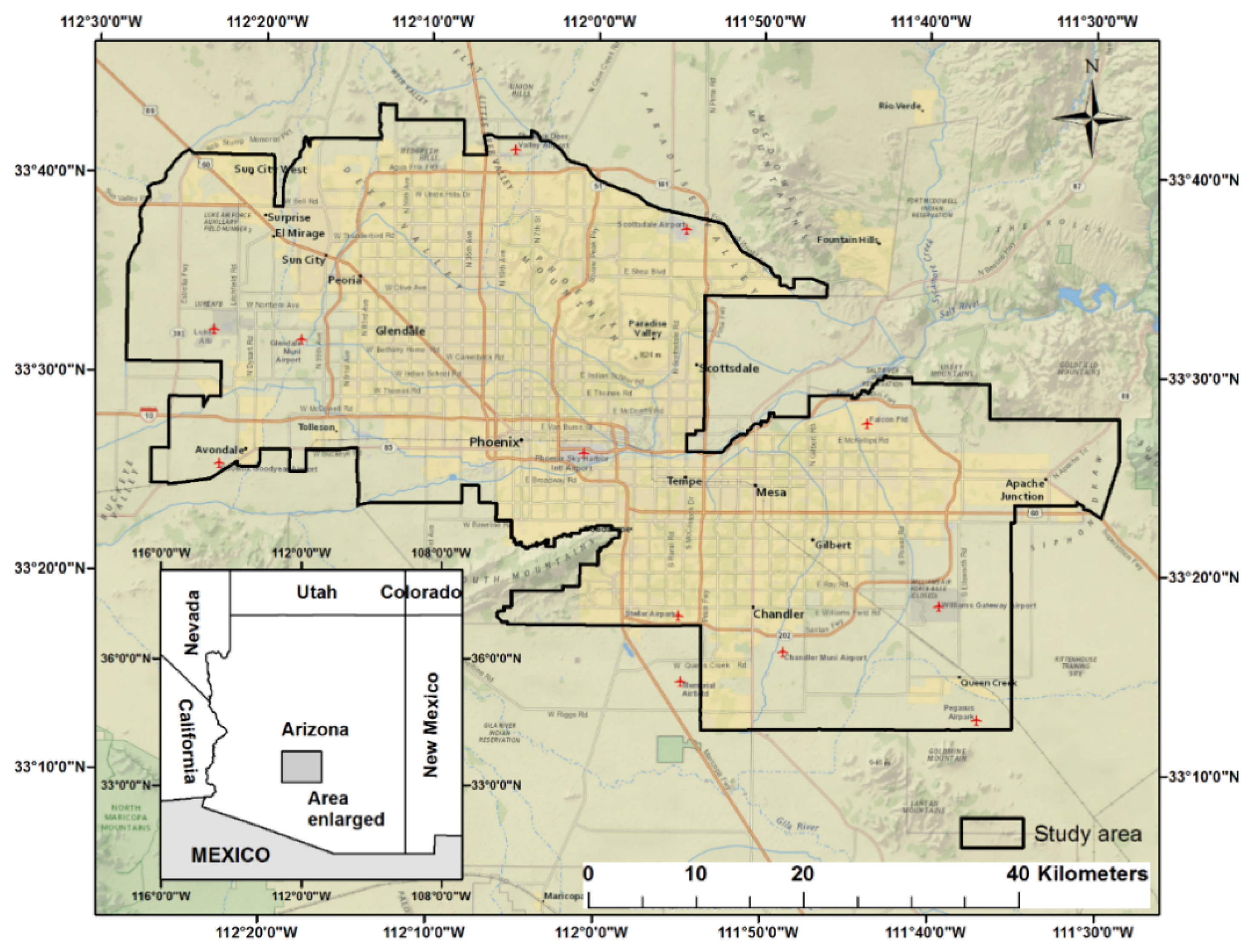
2. Study Area
3. Data and Methods
3.1. Data
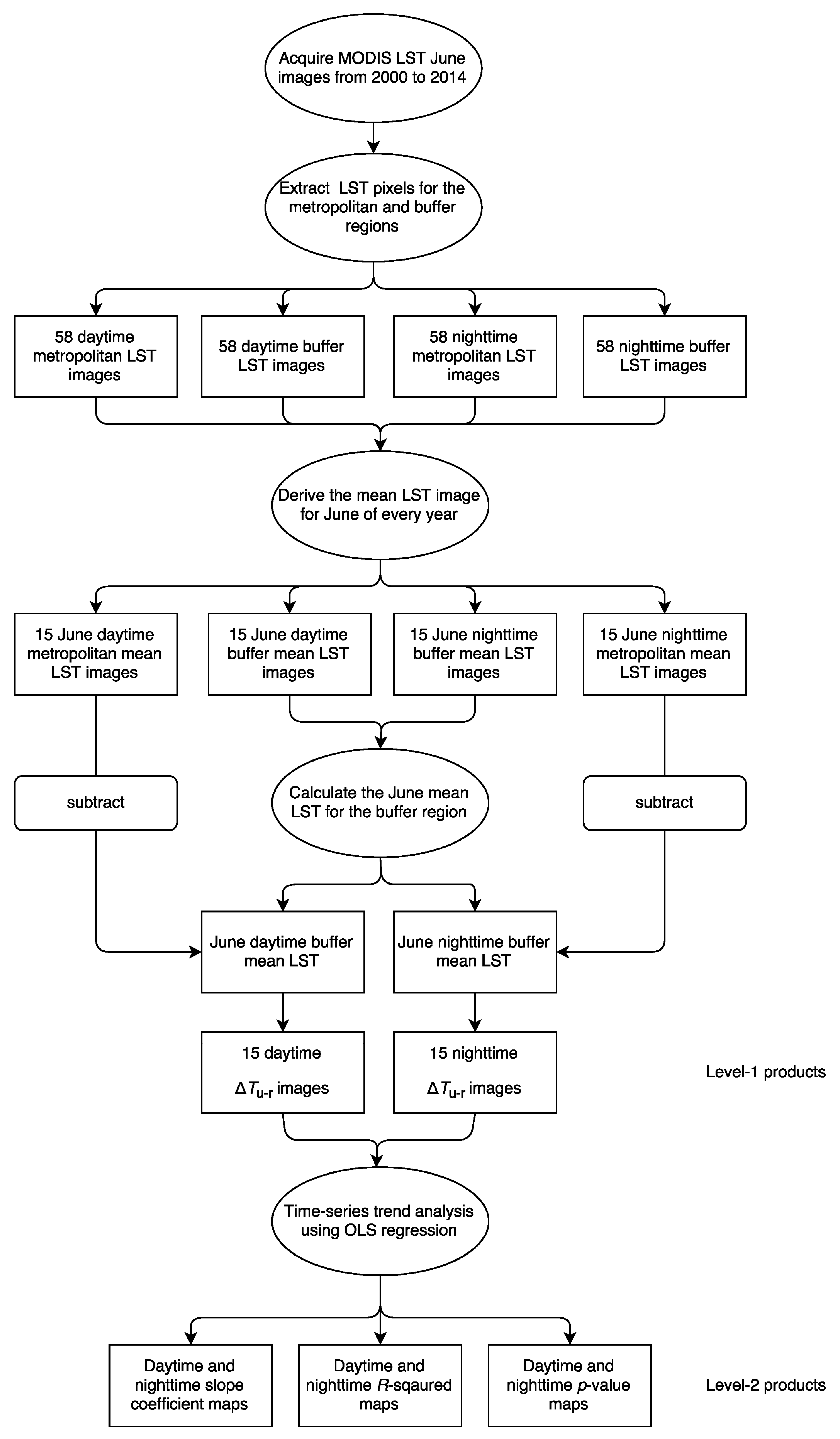
3.2. MODIS LST Image Processing and Data Analysis
3.3. LULC Change Analysis
4. Results
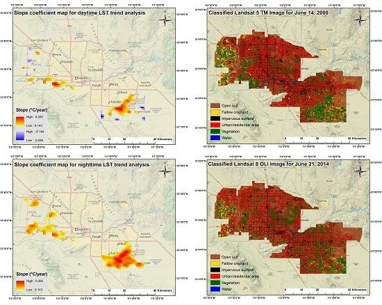
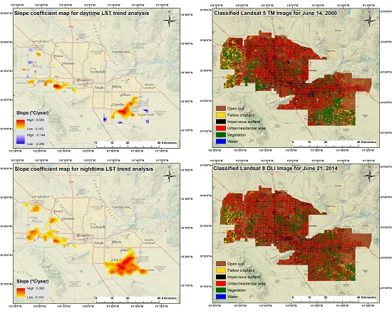
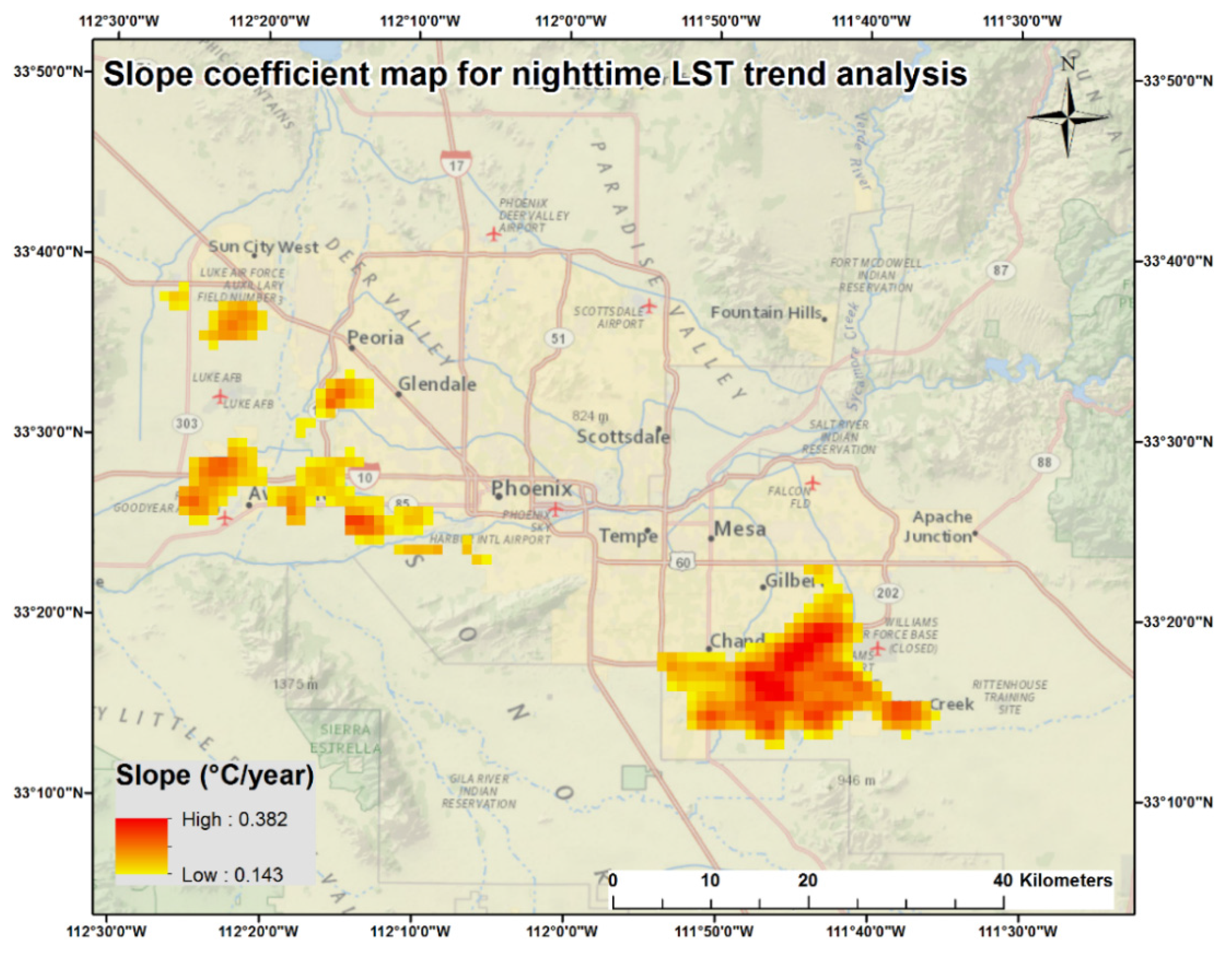
4.1. Ordinary Least Squares Regression Results
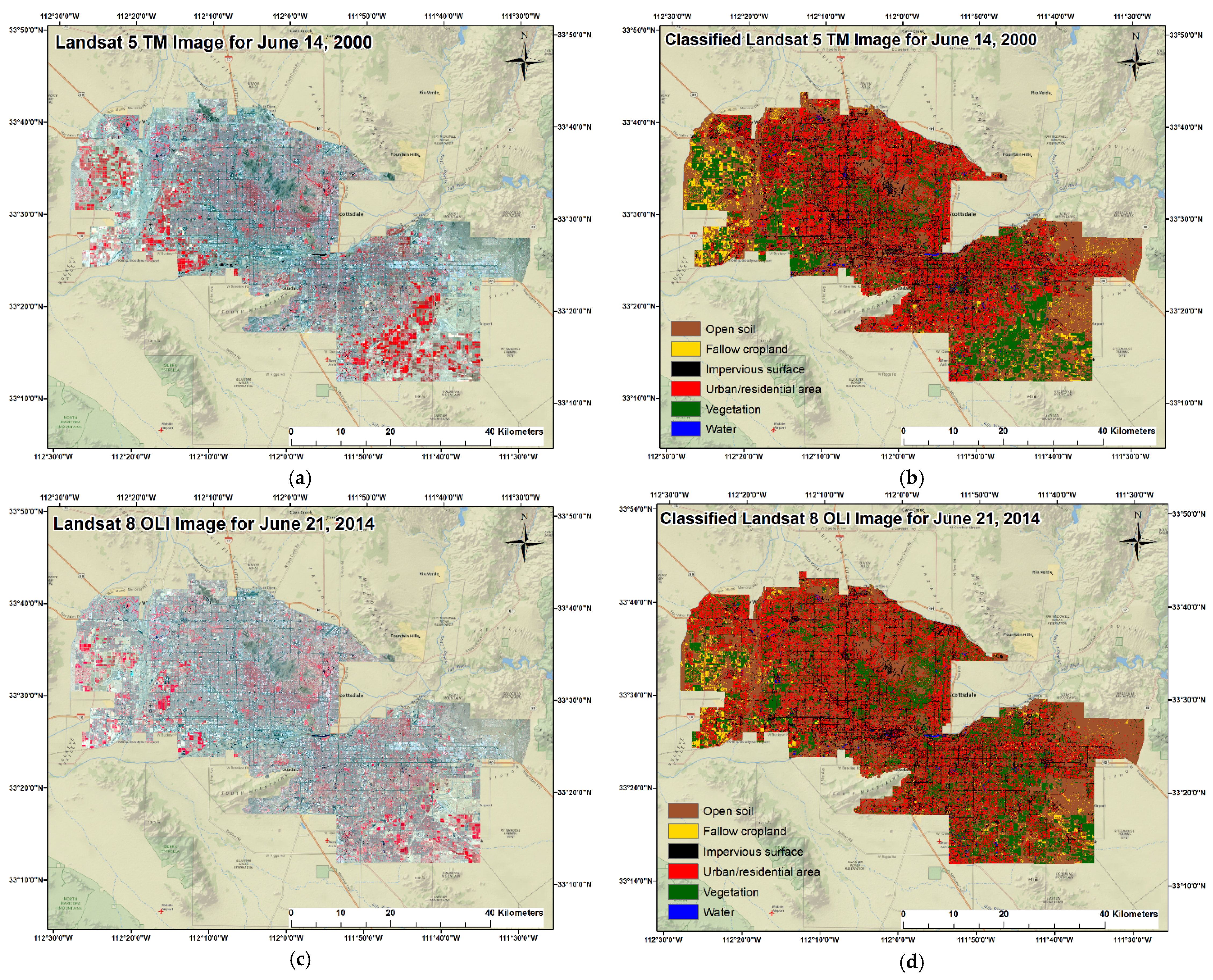
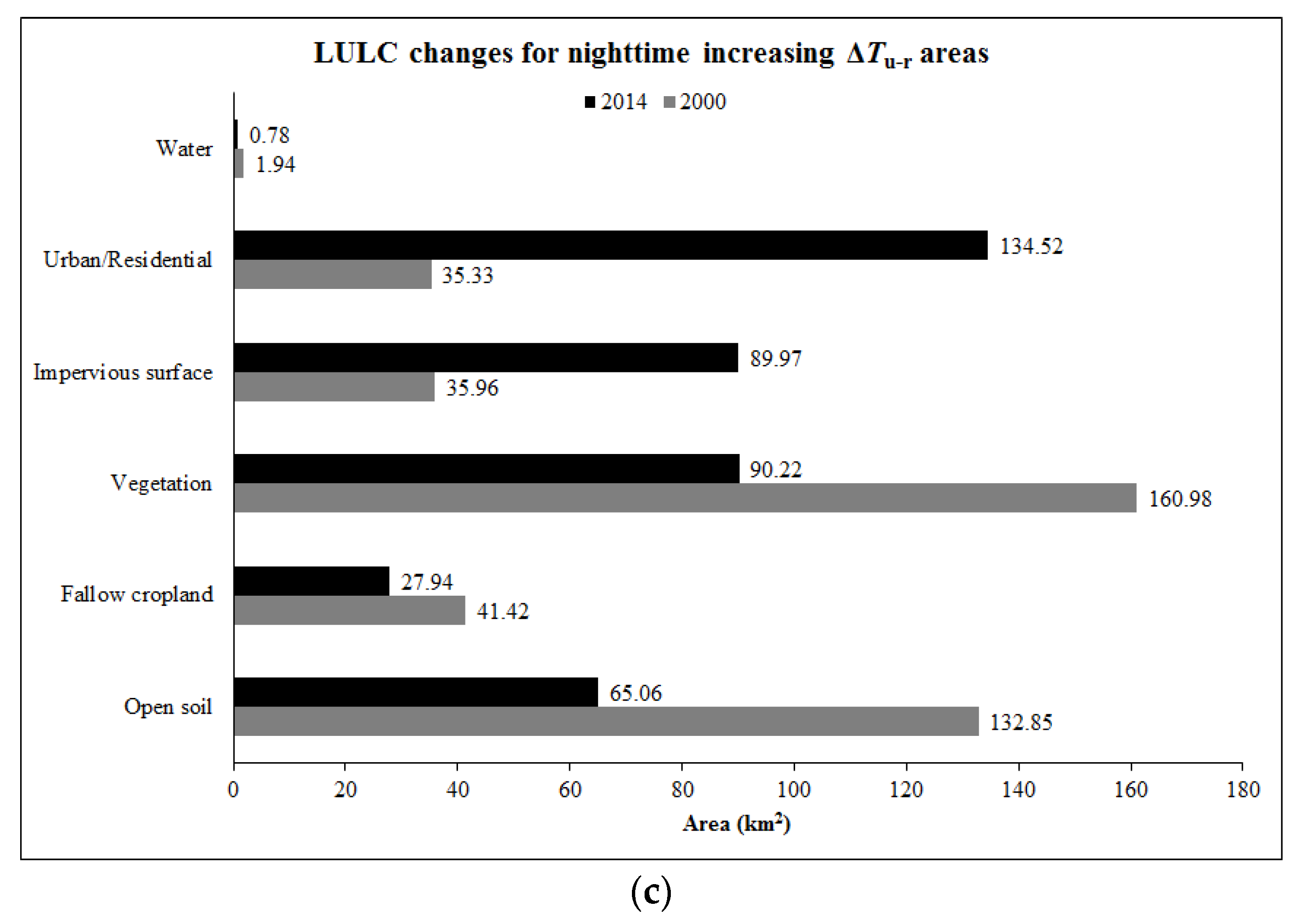
4.2. LULC Change Analysis Results
5. Discussion
6. Conclusions
Acknowledgments
Author Contributions
Conflicts of Interest
References
- Hansen, J.; Ruedy, R.; Glascoe, J.; Sato, M. GISS analysis of surface temperature change. J. Geophys. Res. 1999, 104, 30997–31022. [Google Scholar] [CrossRef]
- Akbari, H.; Pomerantz, M.; Taha, H. Cool surfaces and shade trees to reduce energy use and improve air quality in urban areas. Sol. Energy 2001, 70, 295–310. [Google Scholar] [CrossRef]
- Kolokotroni, M.; Ren, X.; Davies, M.; Mavrogianni, A. London’s urban heat island: Impact on current and future energy consumption in office buildings. Energy Build. 2012, 47, 302–311. [Google Scholar] [CrossRef]
- Guhathakurta, S.; Gober, P. The impact of the Phoenix urban heat island on residential water use. J. Am. Plan. Assoc. 2007, 73, 317–329. [Google Scholar] [CrossRef]
- Brazel, A.; Gober, P.; Lee, S.-J.; Grossman-Clarke, S.; Zehnder, J.; Hedquist, B.; Comparri, E. Determinants of changes in the regional urban heat island in metropolitan Phoenix (Arizona, USA) between 1990 and 2004. Clim. Res. 2007, 33, 171–182. [Google Scholar] [CrossRef]
- Taha, H.; Kalkstein, L.S.; Sheridan, S.C.; Wong, E. The potential of urban environmental control in alleviating heat-wave health effects in five US regions. In Proceedings of the 16th Conference on Biometeorology and Aerobiology, American Meteorological Society, Vancouver, BC, Canada, 23–27 August 2004.
- Taha, H.; Douglas, S.; Haney, J. The UAM sensitivity analysis: The 26–28 August 1987 oxidant episode. In Analysis of Energy Efficiency and Air Quality in the South Coast Air Basin—Phase II; Taha, H., Ed.; Lawrence Berkeley Laboratory: Berkeley, CA, USA, 1994; Chapter 1. [Google Scholar]
- Filleul, L.; Cassadou, S.; Médina, S.; Fabres, P.; Lefranc, A.; Eilstein, D.; Le Tertre, A.; Pascal, L.; Chardon, B.; Blanchard, M.; et al. The relation between temperature, ozone, and mortality in nine French cities during the heat wave of 2003. Environ. Health Perspect. 2006, 114, 1344–1347. [Google Scholar] [CrossRef]
- Balling, R.C., Jr.; Brazil, S.W. Time and space characteristics of the Phoenix urban heat island. J. Ariz.-Nev. Acad. Sci. 1987, 21, 75–81. [Google Scholar]
- Lee, T.-W.; Lee, J.Y.; Wang, Z.-H. Scaling of the urban heat island intensity using time-dependent energy balance. Urban Clim. 2012, 2, 16–24. [Google Scholar] [CrossRef]
- Yuan, F.; Bauer, M.E. Comparison of impervious surface area and normalized difference vegetation index as indicators of surface urban heat island effects in Landsat imagery. Remote Sens. Environ. 2007, 106, 375–386. [Google Scholar] [CrossRef]
- Chen, X.-L.; Zhao, H.-M.; Li, P.-X.; Yin, Z.-Y. Remote sensing image-based analysis of the relationship between urban heat island and land use/cover changes. Remote Sens. Environ. 2006, 104, 133–146. [Google Scholar] [CrossRef]
- Kato, S.; Yamaguchi, Y. Analysis of urban heat-island effect using ASTER and ETM+ data: Separation of anthropogenic heat discharge and natural heat radiation from sensible heat flux. Remote Sens. Environ. 2005, 99, 44–54. [Google Scholar] [CrossRef]
- Nichol, J.E.; Fung, W.Y.; Lam, K.; Wong, M.S. Urban head island diagnosis using ASTER satellite images and “in situ” air temperature. Atmos. Res. 2009, 94, 276–284. [Google Scholar] [CrossRef]
- Liu, L.; Zhang, Y. Urban heat island analysis using the Landsat TM data and ASTER data: A case study in Hong Kong. Remote Sens. 2011, 3, 1535–1552. [Google Scholar] [CrossRef]
- Myint, S.W.; Wentz, E.A.; Brazel, A.J.; Quattrochi, D.A. The impact of distinct anthropogenic and vegetation features on urban warming. Landsc. Ecol. 2013, 28, 959–978. [Google Scholar] [CrossRef]
- Imhoff, M.L.; Zhang, P.; Wolfe, R.E.; Bounoua, L. Remote sensing of the urban heat island effect across biomes in the continental USA. Remote Sens. Environ. 2010, 114, 504–513. [Google Scholar] [CrossRef]
- Zheng, B.; Myint, S.W.; Fan, C. Spatial configuration of anthropogenic land cover impacts on urban warming. Landsc. Urban Plan. 2014, 130, 104–111. [Google Scholar] [CrossRef]
- Gober, P.; Brazil, A.; Quay, R.; Myint, S.; Grossman-Clarke, S.; Miller, A.; Rossi, S. Using watered landscape to manipulate urban heat island effects: How much water will it take to cool Phoenix? J. Am. Plan. Assoc. 2009, 76, 109–121. [Google Scholar] [CrossRef]
- Rossi, F.; Pisello, A.L.; Nicolini, A.; Filipponi, M.; Palombo, M. Analysis of retro-reflective surfaces for urban heat island mitigation: A new analytical model. Appl. Energy 2014, 114, 621–631. [Google Scholar] [CrossRef]
- Santamouris, M.; Synnefa, A.; Karlessi, T. Using advanced cool materials in the urban built environment to mitigate heat islands and improve thermal comfort conditions. Sol. Energy 2011, 85, 3085–3102. [Google Scholar] [CrossRef]
- Uemoto, K.L.; Sato, N.M.N.; John, V.M. Estimating thermal performance of cool colored paints. Energy Build. 2010, 42, 17–22. [Google Scholar] [CrossRef]
- Jo, J.H.; Carlson, J.D.; Golden, J.S.; Bryan, H. An integrated empirical and modeling methodology for analyzing solar reflective roof technologies on commercial buildings. Build. Environ. 2010, 45, 453–460. [Google Scholar] [CrossRef]
- Yang, J.; Wang, Z.-H.; Kaloush, K. E. Environmental impacts on reflective materials: Is high albedo a “silver bullet” for mitigating urban heat island? Renew. Sustain. Energy Rev. 2015, 47, 830–843. [Google Scholar] [CrossRef]
- U.S. Census Bureau. Available online: http://www.census.gov/popest/data/metro/totals/2013/index.html (accessed on 29 January 2016).
- U.S. Climate Data. Available online: http://www.usclimatedata.com/climate/phoenix/arizona/united-states/usaz0166 (accessed on 29 January 2016).
- Peng, S.; Piao, S.; Ciais, P.; Friedlingstein, P.; Ottle, C.; Bréon, F.-M.; Nan, H.; Zhou, L.; Myneni, R.B. Surface Urban Heat Island across 419 Global Big Cities. Environ. Sci. Technol. 2012, 46, 696–703. [Google Scholar] [CrossRef] [PubMed]
- Schwarz, N.; Lautenbach, S.; Seppelt, R. Exploring indicators for quantifying surface urban heat islands of European cities with MODIS land surface temperatures. Remote Sens. Environ. 2011, 115, 3175–3186. [Google Scholar] [CrossRef]
- Tomlinson, C.J.; Chapman, L.; Thornes, J.E.; Baker, C.J. Derivation of Birmingham’s summer surface urban heat island from MODIS satellite images. Int. J. Climatol. 2010, 32, 214–224. [Google Scholar] [CrossRef]
- Rajasekar, U.; Weng, Q. Urban heat island monitoring and analysis using a non-parametric model: A case study of Indianapolis. ISPRS J. Photogramm. Remote Sens. 2009, 64, 86–96. [Google Scholar] [CrossRef]
- Cheval, S.; Dumitrescu, A. The July urban heat island of Bucharest as derived from MODIS images. Theor. Appl. Climatol. 2009, 96, 145–153. [Google Scholar] [CrossRef]
- Tran, H.; Uchihama, D.; Ochi, S.; Yasuoka, Y. Assessment with satellite data of the urban heat island effects in Asian mega cities. Int. J. Appl. Earth Obs. Geoinform. 2006, 8, 34–48. [Google Scholar] [CrossRef]
- Brazel, A.J.; Selover, N.; Vose, R.; Heisler, G. Tale of two climates—Baltimore and Phoenix urban LTER sites. Clim. Res. 2000, 15, 123–135. [Google Scholar] [CrossRef]
- Oke, T.R. The heat island of the urban boundary layer: Characteristics, causes and effects. In Wind Climate in Cities; Cermak, J.E., Davenport, A.G., Plate, E.J., Viegas, D.X., Eds.; Kluwer Academic: Dordrecht, The Netherlands, 1995; pp. 81–107. [Google Scholar]
- Steward, I.D.; Oke, T.R. Local climate zones for urban temperature studies. Bull. Am. Meteorol. Soc. 2012, 93, 1879–1900. [Google Scholar] [CrossRef]
- Wang, Z.-H.; Bou-Zeid, E.; Smith, J.A. A coupled energy transport and hydrological model for urban canopies with evaluation using a wireless sensor network. Q. J. R. Meteorol. Soc. 2013, 139, 1643–1657. [Google Scholar] [CrossRef]
- Schatz, J.; Kucharik, C.J. Seasonality of the urban heat island effect in Madison, Wisconsin. J. Appl. Meteorol. Clim. 2014, 53, 2371–2386. [Google Scholar] [CrossRef]
- Oke, T.R. The energetic basis of the urban heat island. Q. J. R. Meteorol. Soc. 1982, 108, 1–24. [Google Scholar] [CrossRef]
- Weng, Q. A remote sensing GIS evaluation of urban expansion and its impact on surface temperature in the Zhujiang Delta, China. Int. J. Remote Sens. 2001, 22, 1999–2014. [Google Scholar]
- Bouyer, J.; Musy, M.; Huang, Y.; Athamena, K. Mitigating urban heat island effect by urban design: Forms and materials. In Proceedings of the Fifth Urban Research Symposium 2009, World Bank: Cities and Climate Change: Responding to an Urgent Agenda, Marseille, France, 28–29 June 2009; pp. 1–15.
- Lu, J.; Li, C.; Yu, C.; Jin, M.; Dong, S. Regression analysis of the relationship between urban heat island effect and urban canopy characteristics in a mountainous city, Chongqing. Indoor Built Environ. 2012, 21, 821–836. [Google Scholar] [CrossRef]
- Song, J.; Wang, Z.-H. Interfacing the urban land-atmosphere system through coupled urban canopy and atmospheric models. Bound. Layer Meteorol. 2015, 154, 427–448. [Google Scholar] [CrossRef]
- Golden, J.S. The built environment induced urban heat island effect in rapidly urbanizing arid regions—A sustainable urban engineering complexity. Environ. Sci. 2004, 1, 321–349. [Google Scholar] [CrossRef]
- Mills, G. Urban climatology and urban design. In Proceedings of the 15th ICB & ICUC, Sydney, Australia, 8–12 November 1999.
- Bohnenstengel, S.I.; Evans, S.; Clark, P.A.; Belcher, S.E. Simulations of the Landon urban heat island. Q. J. R. Meteorol. Soc. 2011, 137, 1625–1640. [Google Scholar] [CrossRef]
- Pal, S.; Xueref-Remy, I.; Ammoura, L.; Chazette, P.; Gibert, F.; Royer, P.; Dieudonné, E.; Dupont, J.-C.; Haeffelin, M.; Lac, C.; et al. Spatio-temporal variability of the atmospheric boundary layer depth over the Paris agglomeration: An assessment of the impact of the urban heat island intensity. Atmos. Environ. 2012, 63, 261–275. [Google Scholar] [CrossRef]
- Lac, C.; Donnelly, R.P.; Masson, V.; Pal, S.; Riette, S.; Donier, S.; Queguiner, S.; Tanguy, G.; Ammoura, L.; Xueref-Remy, I. CO2 dispersion modelling over Paris region within the CO2-MEGAPARIS project. Atmos. Chem. Phys. 2013, 13, 4941–4961. [Google Scholar] [CrossRef]
- Rosenfeld, A.H.; Akbari, H.; Bretz, S.; Fishman, B.L.; Kurn, D.M.; Sailor, D.; Taha, H. Mitigation of urban heat islands: Materials, utility programs, updates. Energy Build. 1995, 22, 255–265. [Google Scholar] [CrossRef]
- Ca, V.T.; Asaeda, T.; Abu, E.M. Reductions in air-conditioning energy caused by a nearby park. Energy Build. 1998, 29, 83–92. [Google Scholar] [CrossRef]
- Ashie, Y.; Thanh, V.C.; Asaeda, T. Building canopy model for the analysis of urban climate. J. Wind Eng. Ind. Aerod. 1999, 81, 237–248. [Google Scholar] [CrossRef]
- Tong, H.; Walton, A.; Sang, J.; Chan, J.C.L. Numerical simulation of the urban boundary layer over the complex terrain of Hong Kong. Atmos. Environ. 2005, 39, 3549–3563. [Google Scholar] [CrossRef]
- Yu, C.; Hien, W.N. Thermal benefits of city parks. Energy Build. 2006, 38, 105–120. [Google Scholar] [CrossRef]
- Yang, J.; Wang, Z.-H. Optimizing urban irrigation schemes for the trade-off between energy and water consumption. Energy Build. 2015, 107, 335–344. [Google Scholar] [CrossRef]
- Taha, H. Urban climates and heat islands: Albedo, evapotranspiration, and anthropogenic heat. Energy Build. 1997, 25, 99–103. [Google Scholar] [CrossRef]
- Lo, C.P.; Quattrochi, D.A.; Luvall, J.C. Application of high-resolution thermal infrared remote sensing and GIS to assess the urban heat island effect. Int. J. Remote Sens. 1997, 18, 287–304. [Google Scholar] [CrossRef]


| LULC Types | 2000 Landsat 5 TM Image | 2014 Landsat 8 OLI Image | ||
|---|---|---|---|---|
| Producer’s Accuracy | User’s Accuracy | Producer’s Accuracy | User’s Accuracy | |
| Open soil | 79% | 83% | 77% | 85% |
| Fallow cropland | 79% | 80% | 84% | 76% |
| Urban/Residential | 83% | 86% | 79% | 85% |
| Vegetation | 100% | 90% | 98% | 94% |
| Impervious surface | 80% | 85% | 78% | 81% |
| Water | 97% | 92% | 97% | 89% |
| Overall accuracy | 86% | 85% | ||
| Kappa coefficient | 0.83 | 0.82 | ||
| Open Soil | Fallow Cropland | Urban/Residential | Vegetation | Impervious Surface | Water | |
|---|---|---|---|---|---|---|
| Slope (daytime) | 0.4287 * (0.0000) | 0.0564 (0.4016) | 0.1136 (0.0905) | −0.6087 * (0.0000) | 0.3631 * (0.0000) | 0.0253 (0.7076) |
| Slope (nighttime) | 0.1237 * (0.0122) | −0.1463 * (0.0030) | 0.3009* (0.0000) | −0.4157 * (0.0000) | 0.3399 * (0.0000) | 0.0209 (0.6729) |
© 2016 by the authors; licensee MDPI, Basel, Switzerland. This article is an open access article distributed under the terms and conditions of the Creative Commons by Attribution (CC-BY) license (http://creativecommons.org/licenses/by/4.0/).
Share and Cite
Wang, C.; Myint, S.W.; Wang, Z.; Song, J. Spatio-Temporal Modeling of the Urban Heat Island in the Phoenix Metropolitan Area: Land Use Change Implications. Remote Sens. 2016, 8, 185. https://0-doi-org.brum.beds.ac.uk/10.3390/rs8030185
Wang C, Myint SW, Wang Z, Song J. Spatio-Temporal Modeling of the Urban Heat Island in the Phoenix Metropolitan Area: Land Use Change Implications. Remote Sensing. 2016; 8(3):185. https://0-doi-org.brum.beds.ac.uk/10.3390/rs8030185
Chicago/Turabian StyleWang, Chuyuan, Soe W. Myint, Zhihua Wang, and Jiyun Song. 2016. "Spatio-Temporal Modeling of the Urban Heat Island in the Phoenix Metropolitan Area: Land Use Change Implications" Remote Sensing 8, no. 3: 185. https://0-doi-org.brum.beds.ac.uk/10.3390/rs8030185