
Mosaicking of Unmanned Aerial Vehicle Imagery in the Absence of Camera Poses

Abstract
:
1. Introduction
- (1)
- The camera lens has no evident distortion (or, in cases of significant distortion, lens distortion coefficients are available).
- (2)
- The ground is approximately planar.
2. Related Work
3. Methodology
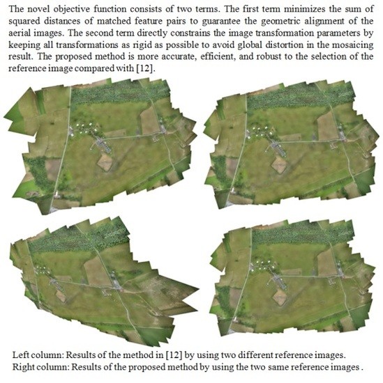
3.1. Objective Function
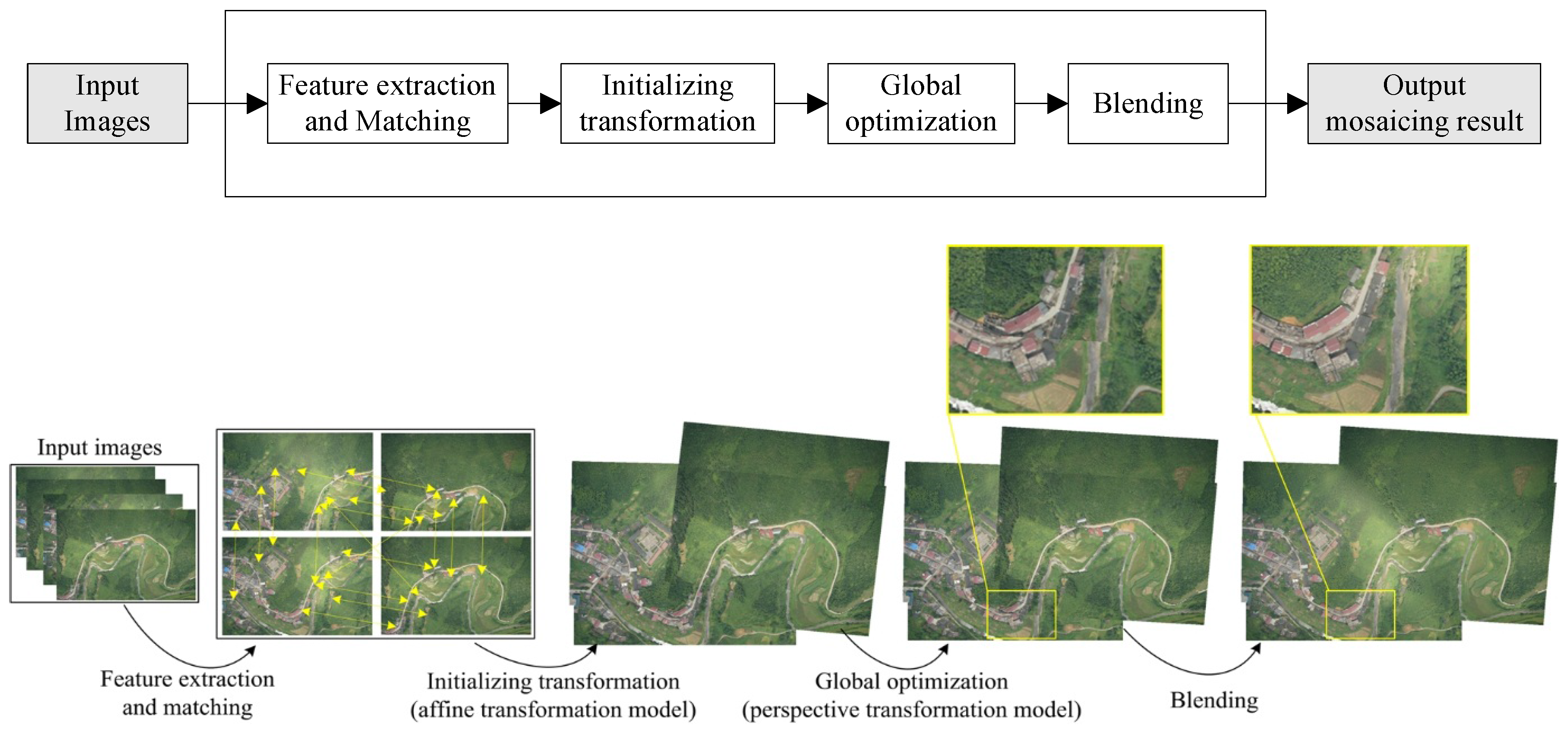
3.2. Mosaicking Work-Flow
3.2.1. Feature Extraction and Matching
3.2.2. Initialization of the Transformation Parameters
3.2.3. Global Optimization
3.2.4. Blending
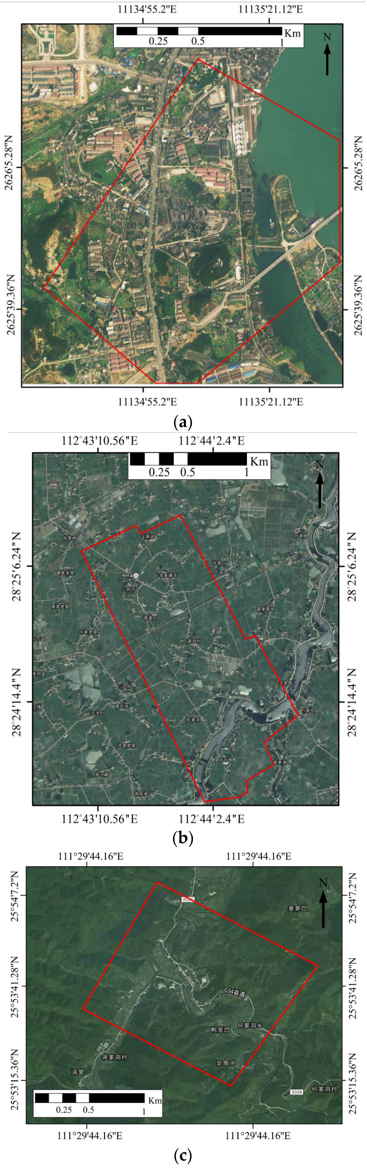
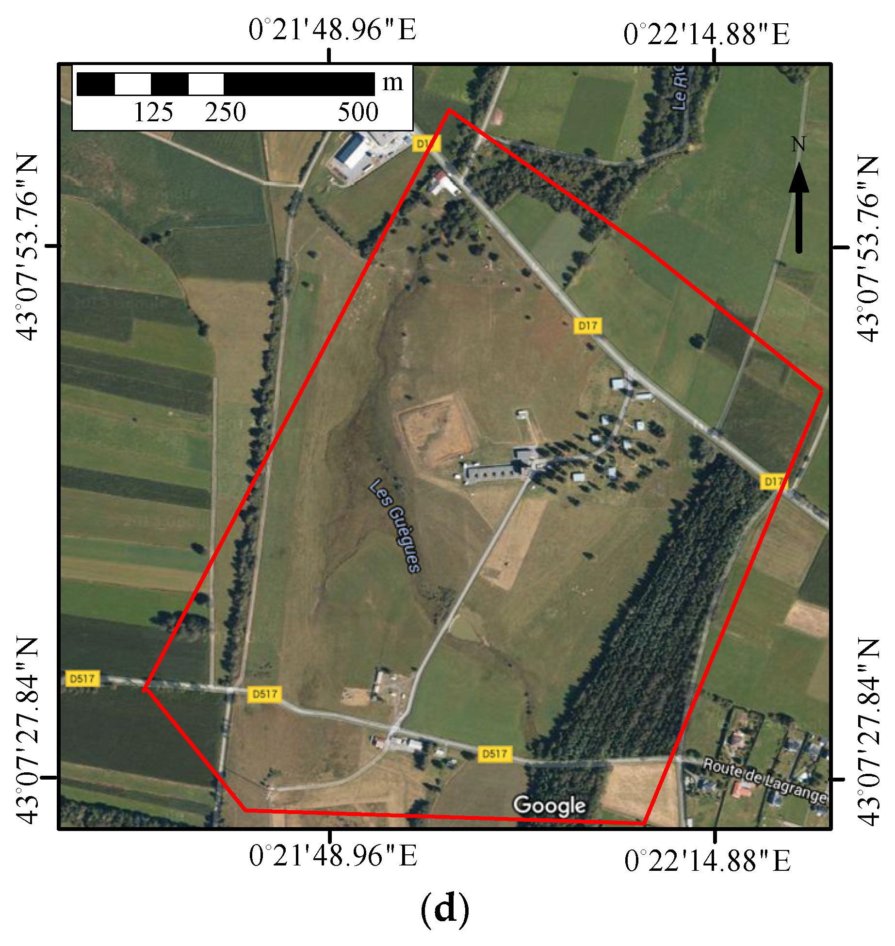
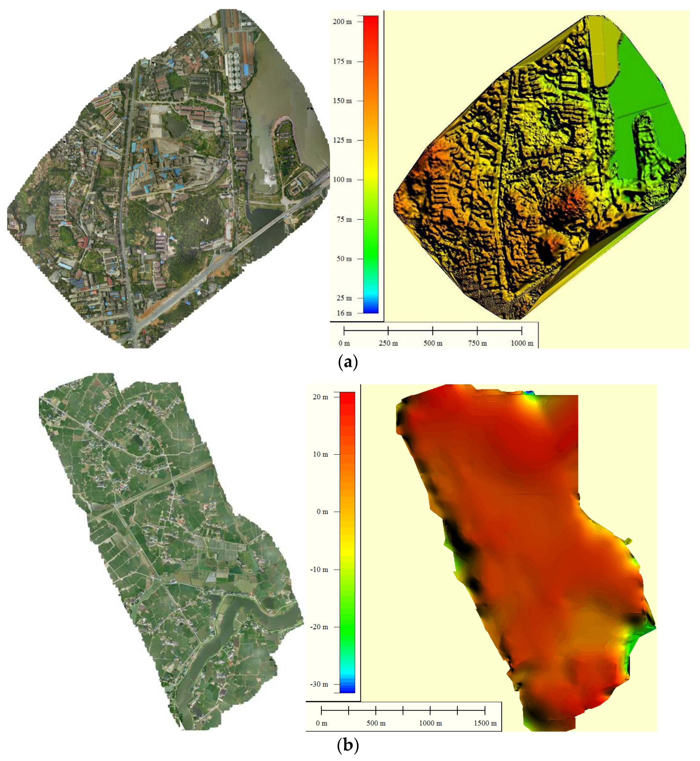
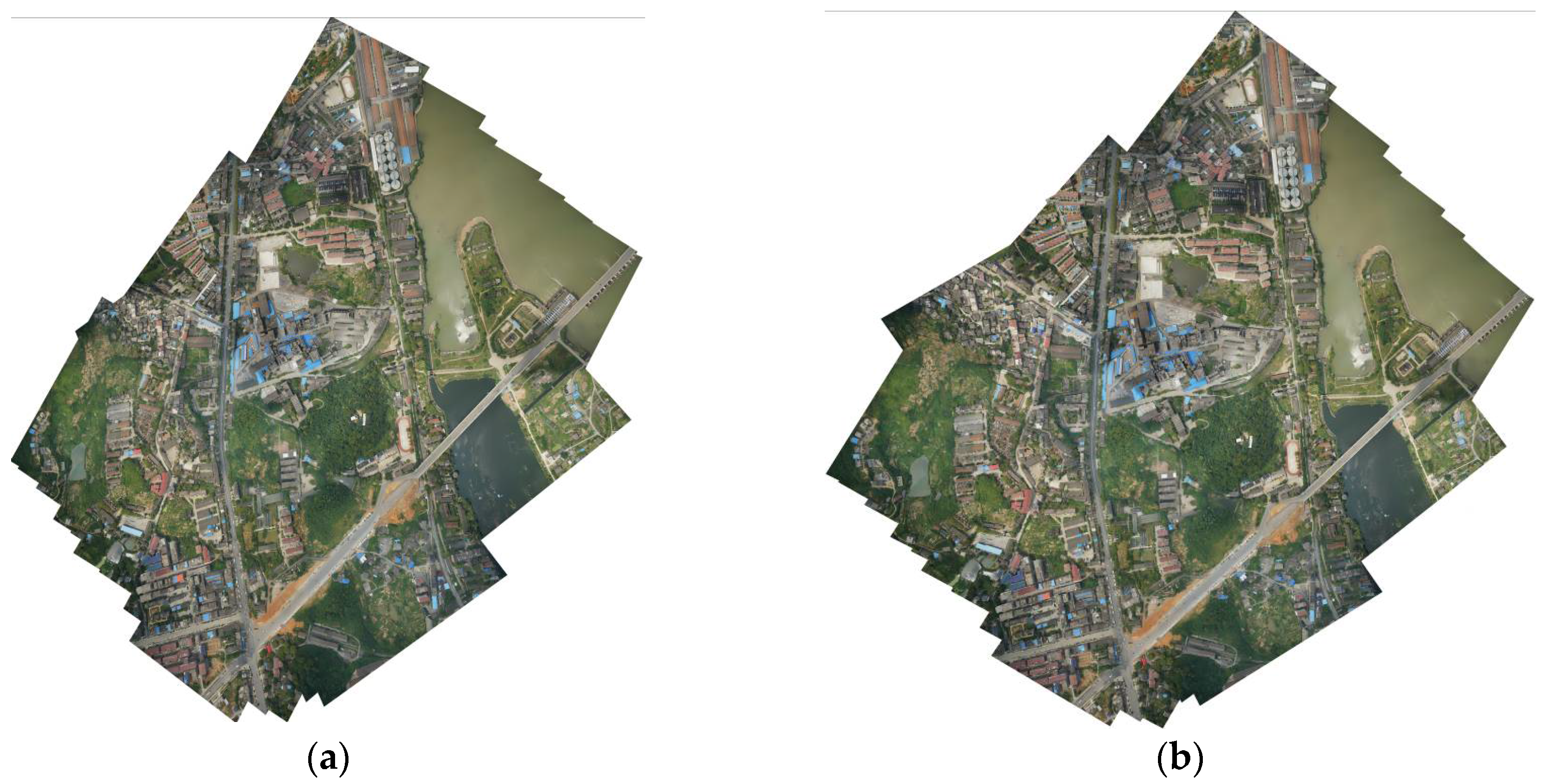
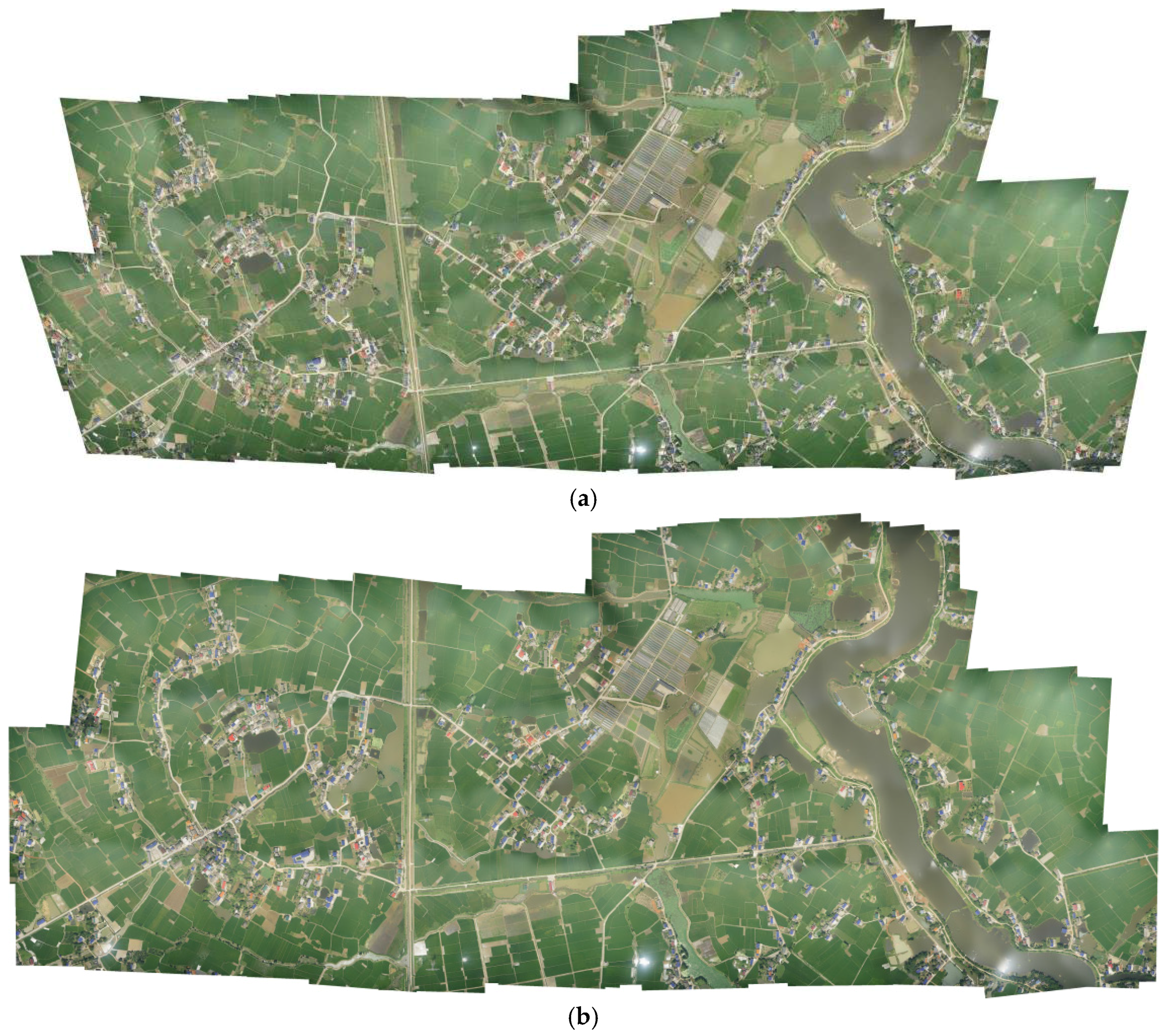
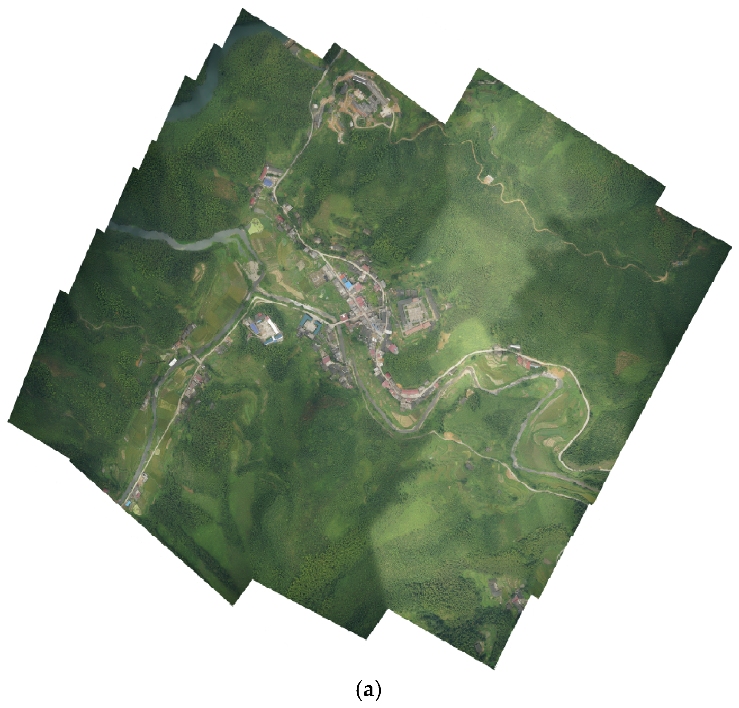
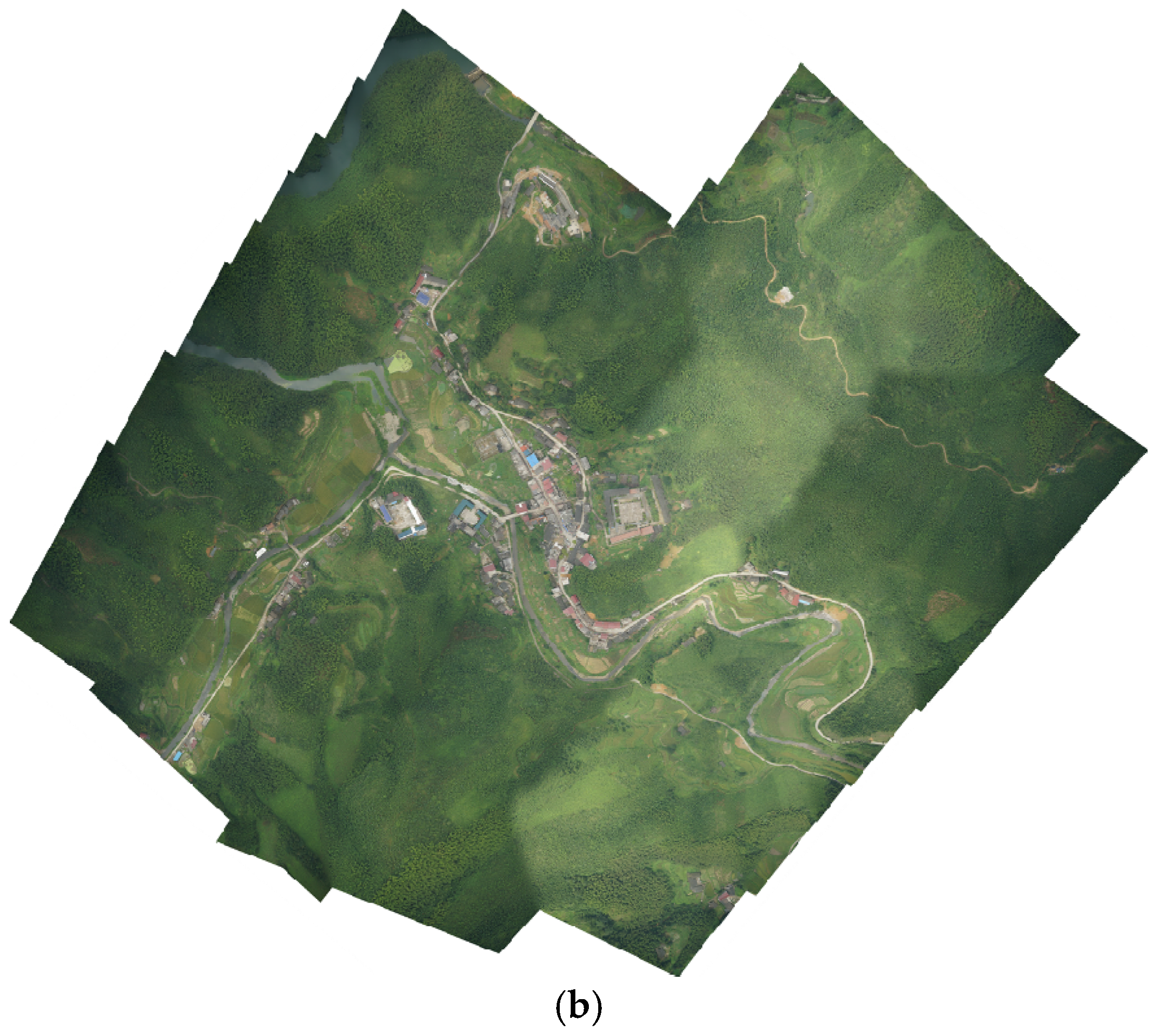
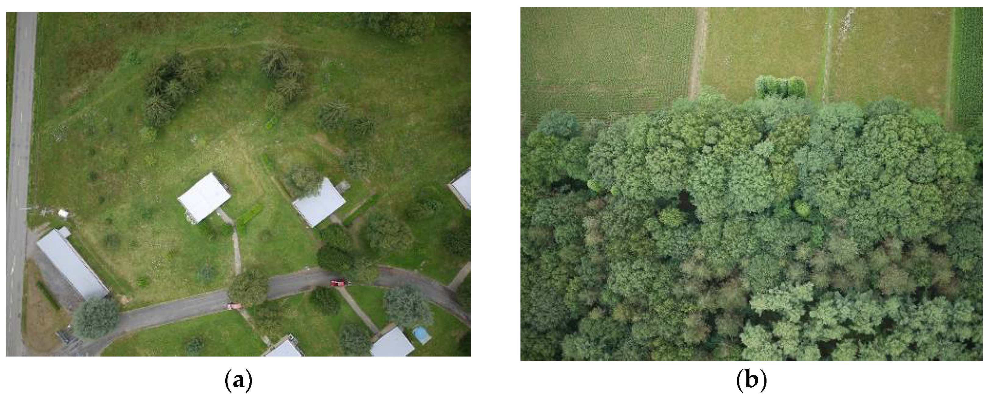
4. Datasets
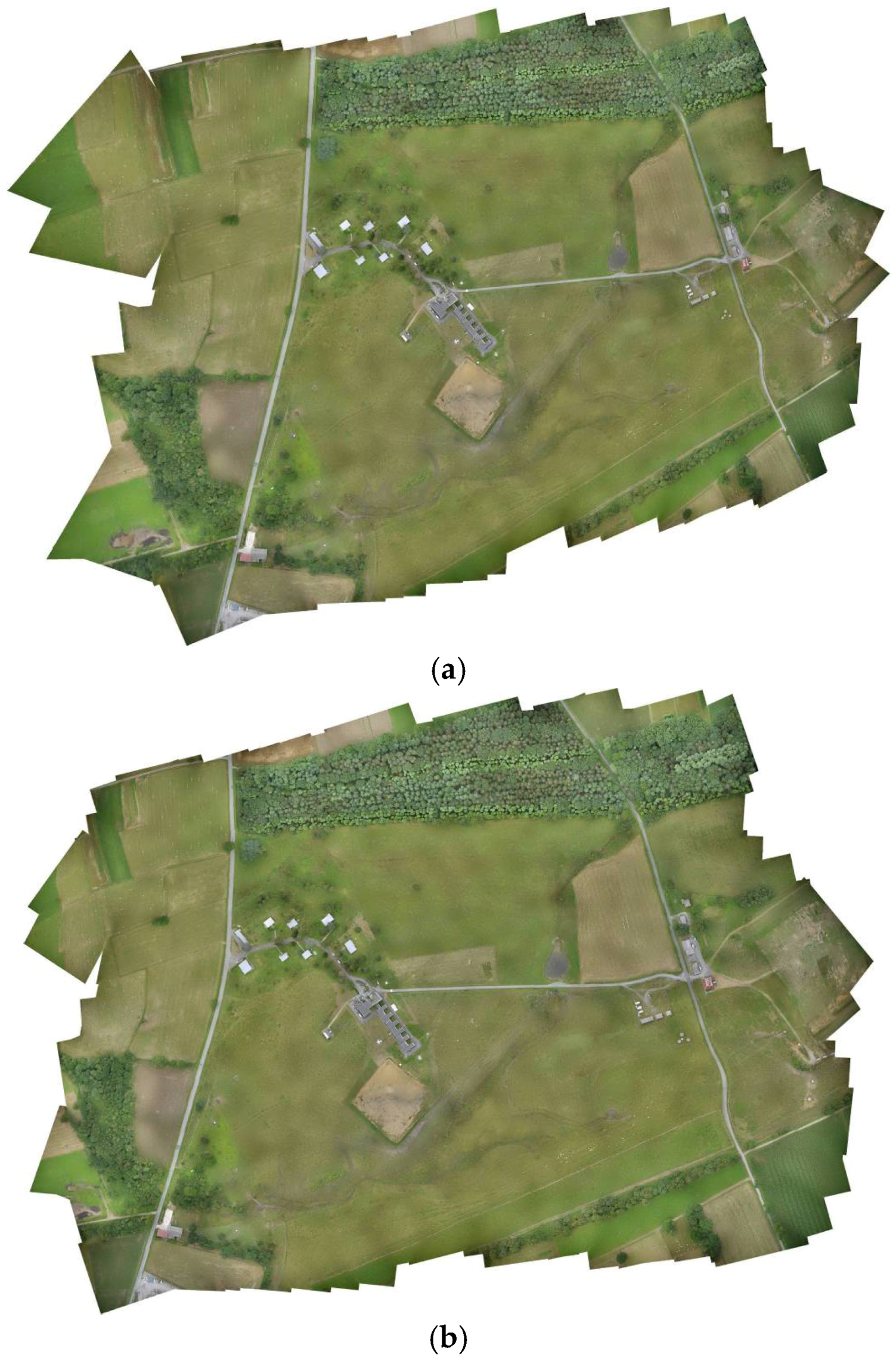
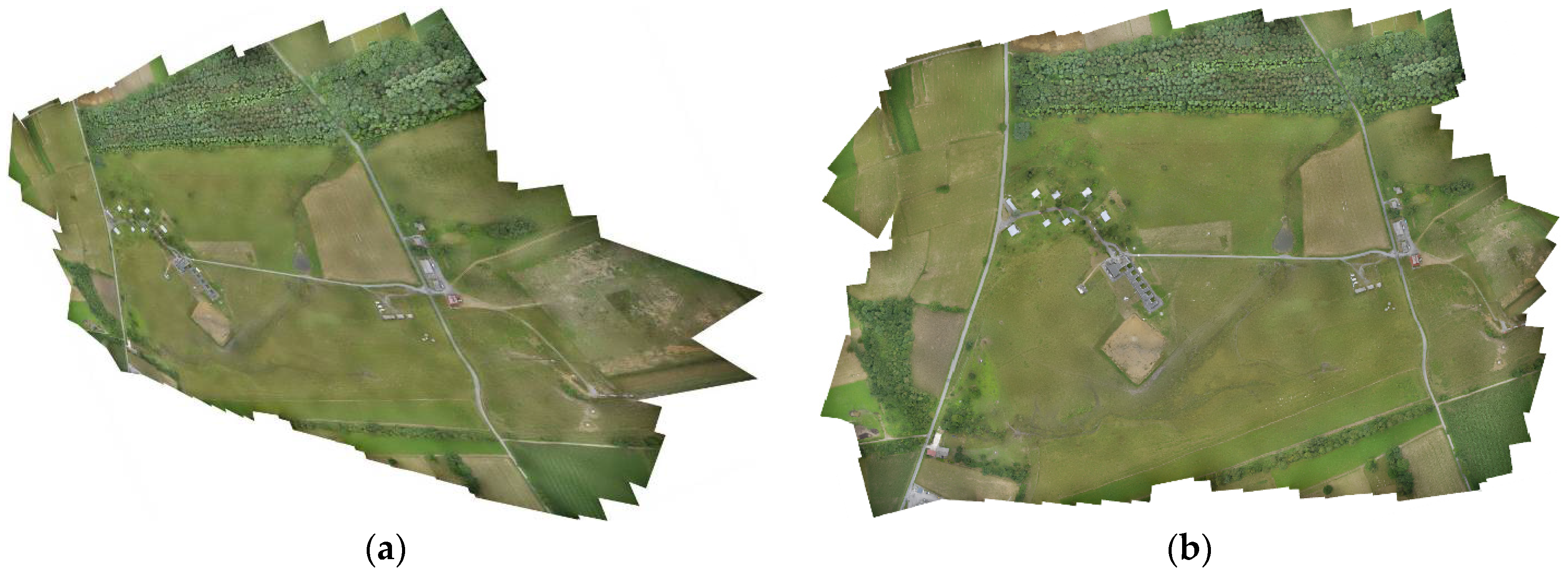
5. Results and Discussion
5.1. Accuracy
5.2. Efficiency
5.3. Impact of the Reference Image
5.4. Impact of Variations in Terrain Elevation
6. Conclusions
Acknowledgments
Author Contributions
Conflicts of Interest
References
- Bryson, M.; Reid, A.; Ramos, F.; Sukkarieh, S. Airborne vision-based mapping and classification of large farmland environments. J. Field Robot. 2010, 5, 632–655. [Google Scholar] [CrossRef]
- Heinze, N.; Esswein, M.; Krüger, W.; Saur, G. Automatic image exploitation system for small UAVs. Proc. SPIE 6946 2008. [Google Scholar] [CrossRef]
- Zhou, G. Near real-time orthorectification and mosaic of small UAV video flow for time-critical event response. IEEE Trans. Geosci. Remote Sens. 2009, 3, 739–747. [Google Scholar] [CrossRef]
- Chen, C.S.; Chen, Y.T.; Huang, F. Stitching and reconstruction of linear-pushbroom panoramic images for planar scenes. In Proceedings of the European Conference on Computer Vision, Prague, Czech Republic, 11–14 May 2004.
- Se, S.; Firoozfam, P.; Goldstein, N.; Wu, L.; Dutkiewicz, M.; Pace, P.; Naud, J.P. Automated UAV-based mapping for airborne reconnaissance and video exploitation. Proc. SPIE 7307 2009. [Google Scholar] [CrossRef]
- Stephen, H. Geocoded terrestrial mosaics using pose sensors and video registration. In Proceedings of the IEEE Computer Society Conference on Computer Vision and Pattern Recognition, Kauai, HI, USA, 8–14 December 2001.
- Yahyanejad, S.; Wischounig-Strucl, D.; Quaritsch, M.; Rin, B. Incremental mosaicking of images from autonomous small UAVs. In Proceedings of the 7th International Conference on Advanced Video and Signal-Based Surveillance, Boston, MA, USA, 29 August–1 September 2010.
- Turner, D.; Lucieer, A.; Watson, C. An automated technique for generating georectified mosaics from ultra-high resolution unmanned aerial vehicle (UAV) imagery, based on structure from motion (SFM) point clouds. Remote Sens. 2012, 5, 1392–1410. [Google Scholar] [CrossRef]
- Turner, D.; Lucieer, A.; Wallace, L. Direct georeferencing of ultrahigh-resolution UAV imagery. IEEE Trans. Geosci. Remote Sens. 2013, 5, 2738–2745. [Google Scholar] [CrossRef]
- Yahyanejad, S.; Rinner, B. A fast and mobile system for registration of low-altitude visual and thermal aerial images using multiple small-scale UAVs. ISPRS J. Photogramm. Remote Sens. 2015, 104, 189–202. [Google Scholar] [CrossRef]
- Sumner, R.W.; Schmid, J.; Pauly, M. Embedded deformation for shape manipulation. ACM Trans. Graph. 2007, 3, 1–7. [Google Scholar]
- Capel, D.P. Image mosaicing and super-resolution. Ph.D. Thesis, University of Oxford, Oxford, UK, 2001. [Google Scholar]
- Brown, M.; Lowe, D.G. Automatic panoramic image stitching using invariant features. Int. J. Comput. Vis. 2007, 1, 59–73. [Google Scholar] [CrossRef]
- Agarwala, A.; Agrawala, M.; Cohen, M.; Salesin, D.; Szeliski, R. Photographing long scenes with multi-viewpoint panoramas. ACM Trans. Graph. 2006, 25, 853–861. [Google Scholar] [CrossRef]
- Szeliski, R. Image alignment and stitching: A tutorial. Found. Trends Comput. Graph. Vis. 2006, 2, 1–87. [Google Scholar] [CrossRef]
- Caballero, F.; Merino, L.; Ferruz, J.; Ollero, A. Unmanned aerial vehicle localization based on monocular vision and online mosaicking. J. Intell. Robot. Syst. 2009, 4, 323–343. [Google Scholar] [CrossRef]
- Triggs, B.; McLauchlan, P.; Hartley, R.; Fitzgibbon, A.W. Bundle adjustment—A modern synthesis. In Proceedings of the International Workshop on Vision Algorithms, Corfu, Greece, 21–22 September 1999.
- Lin, C.C.; Pankanti, S.U.; Ramamurthy, K.N.; Aravkin, A.Y. Adaptive as-natural-as-possible image stitching. In Proceedings of the IEEE Conference on Computer Vision and Pattern Recognition, Boston, MA, USA, 7–12 June 2015.
- Madsen, K.; Nielsen, H.B.; Tingleff, O. Methods for Non-Linear Least Squares Problems, 2nd ed.; Informatics and Mathematical Modelling, Technical University of Denmark: Lyngby, Denmark, 2004; pp. 24–29. [Google Scholar]
- Lourakis, M.I.A. Sparse non-linear least squares optimization for geometric vision. In Proceedings of the European Conference on Computer Vision, Hersonissos, Crete, Greece, 5–11 September 2010.
- Lowe, D.G. Distinctive image features from scale-invariant key points. Int. J. Comput. Vis. 2004, 2, 91–110. [Google Scholar] [CrossRef]
- Muja, M.; Lowe, D.G. Fast approximate nearest neighbors with automatic algorithm configuration. In Proceedings of the International Conference on Computer Vision Theory and Applications (VISAPP’09), Lisboa, Portugal, 5–8 February 2009.
- Fischler, M.; Bolles, R. Random sample consensus: A paradigm for model fitting with application to image analysis and automated cartography. Comm. ACM 1981, 6, 381–395. [Google Scholar] [CrossRef]
- Wuhan Intelligent Bird Co., Ltd. Available online: http://www.aibird.com/ (accessed on 18 August 2014).
- DPGrid. Available online: http://www.supresoft.com.cn/ (accessed on 15 July 2015).
- Sample Image Data of Pix4D. Available online: http://www.pix4d.com/ (accessed on 12 February 2015).
- BaiduMap. Available online: http://map.baidu.com/ (accessed on 20 April 2015).
- GoogleMap. Available online: https://maps.google.com/ (accessed on 25 May 2015).


| Proposed Algorithm (m) | Capel’s Method (m) | |||||
|---|---|---|---|---|---|---|
| RMS | MIN | MAX | RMS | MIN | MAX | |
| Dataset 1 | 10.5 | 5.6 | 16.5 | 25.8 | 3.7 | 39.8 |
| Dataset 2 | 5.2 | 0.5 | 12.8 | 22.7 | 1.0 | 42.5 |
| Dataset 3 | 13.4 | 3.9 | 24.6 | 22.5 | 10.8 | 57.2 |
| Dataset 4 | 7.9 | 1.0 | 15.5 | 18.1 | 8.1 | 32.6 |
| Proposed Algorithm (s) | Capel’s Method (s) | |
|---|---|---|
| Dataset 1 | 2.3 | 43.1 |
| Dataset 2 | 35.1 | 1145.5 |
| Dataset 3 | 1.4 | 12.6 |
| Dataset 4 | 36.4 | 1482.6 |
© 2016 by the authors; licensee MDPI, Basel, Switzerland. This article is an open access article distributed under the terms and conditions of the Creative Commons by Attribution (CC-BY) license (http://creativecommons.org/licenses/by/4.0/).
Share and Cite
Xu, Y.; Ou, J.; He, H.; Zhang, X.; Mills, J. Mosaicking of Unmanned Aerial Vehicle Imagery in the Absence of Camera Poses. Remote Sens. 2016, 8, 204. https://0-doi-org.brum.beds.ac.uk/10.3390/rs8030204
Xu Y, Ou J, He H, Zhang X, Mills J. Mosaicking of Unmanned Aerial Vehicle Imagery in the Absence of Camera Poses. Remote Sensing. 2016; 8(3):204. https://0-doi-org.brum.beds.ac.uk/10.3390/rs8030204
Chicago/Turabian StyleXu, Yuhua, Jianliang Ou, Hu He, Xiaohu Zhang, and Jon Mills. 2016. "Mosaicking of Unmanned Aerial Vehicle Imagery in the Absence of Camera Poses" Remote Sensing 8, no. 3: 204. https://0-doi-org.brum.beds.ac.uk/10.3390/rs8030204