Technical Note

Assessing the Accuracy of High Resolution Digital Surface Models Computed by PhotoScan® and MicMac® in Sub-Optimal Survey Conditions

1
Laboratoire Domaines Océaniques—UMR 6538, Université de Bretagne Occidentale, IUEM, Technopôle Brest-Iroise, Rue Dumont D’Urville, F-29280 Plouzané, France
2
Laboratoire de Géologie de Lyon—UMR 5276, Université Claude Bernard Lyon 1, Campus de la Doua, 2 rue Raphaël Dubois, F-69622 Villeurbanne, France
3
CEREMA—Centre d’Etudes et d’expertise sur les Risques, l’Environnement, la Mobilité et l’Aménagement, DTecEMF, F-29280 Plouzané, France
*
Author to whom correspondence should be addressed.
Submission received: 1 February 2016 / Revised: 6 May 2016 / Accepted: 25 May 2016 / Published: 1 June 2016

Abstract

:
For monitoring purposes and in the context of geomorphological research, Unmanned Aerial Vehicles (UAV) appear to be a promising solution to provide multi-temporal Digital Surface Models (DSMs) and orthophotographs. There are a variety of photogrammetric software tools available for UAV-based data. The objective of this study is to investigate the level of accuracy that can be achieved using two of these software tools: Agisoft PhotoScan® Pro and an open-source alternative, IGN© MicMac®, in sub-optimal survey conditions (rugged terrain, with a large variety of morphological features covering a range of roughness sizes, poor GPS reception). A set of UAV images has been taken by a hexacopter drone above the Rivière des Remparts, a river on Reunion Island. This site was chosen for its challenging survey conditions: the topography of the study area (i) involved constraints on the flight plan; (ii) implied errors on some GPS measurements; (iii) prevented an optimal distribution of the Ground Control Points (GCPs) and; (iv) was very complex to reconstruct. Several image processing tests are performed with different scenarios in order to analyze the sensitivity of each software package to different parameters (image quality, numbers of GCPs, etc.). When computing the horizontal and vertical errors within a control region on a set of ground reference targets, both methods provide rather similar results. A precision up to 3–4 cm is achievable with these software packages. The DSM quality is also assessed over the entire study area comparing PhotoScan DSM and MicMac DSM with a Terrestrial Laser Scanner (TLS) point cloud. PhotoScan and MicMac DSM are also compared at the scale of particular features. Both software packages provide satisfying results: PhotoScan is more straightforward to use but its source code is not open; MicMac is recommended for experimented users as it is more flexible.

Graphical Abstract

1. Introduction

Remote sensing techniques combined with data from Unmanned Aerial Vehicles (UAVs) can provide imagery with very high spatial and temporal resolution and covering areas of a few hundred meters. Therefore, UAV-derived 3D models and associated orthophotographs have a great potential for landscape monitoring: coastal management [1,2], precision agriculture [3], erosion assessment, landslides monitoring [4], etc. In the aforementioned applications, mapping small-scale geomorphological features and identifying subtle topographic variations require very high spatial resolution and very high accuracy. The accuracy of the generated orthophoto and 3D model mainly depends on the Structure from Motion (SfM) photogrammetry processing chain and on the raw images.
With the recent developments of small UAVs and the use of Structure from Motion (SfM) algorithms, the rapid acquisition of topographic data at high spatial and temporal resolution is now possible at low costs [2,5,6,7]. The SfM approach is based on the SIFT (Scale-Invariant Feature Transform) image-to-image registration method [8]. In comparison to classic digital photogrammetry, the SfM workflow leads to more automation and is therefore more straightforward for the users [6,9]. Many recent studies deal with performance assessment of methods and software solutions for georeferenced point clouds or Digital Surface Models (DSMs) production; see [10], for instance, for a literature review on this issue. Neitzel and Klonowski [11] compare five software products for 3D point clouds generation. They notice that discrepancies depend on the applied software. Küng et al. [12] report that, with Pix4D® software, the accuracy is strongly influenced by the resolution of the images and the texture and terrain in the scene. Harwin and Lucieer [13] notice that the number and the distribution of the Ground Control Points (GCPs) have a major impact on the accuracy, particularly on the area with topographic relief. They claim that the best distribution of GCPs is an even distribution throughout the focus area with a spacing of 1/5 to 1/10 of the UAV flying height, and that GCPs should be closer in steeper terrain. Anders et al. [14] assess the quality of DSMs computed by PhotoScan for different flight altitudes. All the studies show that the results are highly dependent on the terrain and the topography of the test area and on the quality and distribution of GCPs.
The main objective of this study is to compare the geometric accuracy of the DSM computed from the same sets of images with two different software solutions: PhotoScan® Pro 1.1.5 (an integrated processing chain commercialized by AgiSoft®, which is more and more widely used) and MicMac® (an open-source photogrammetric toolset developed by Institut Géographique National (IGN®), the French National Institute of Geographic and Forestry Information). In this perspective, a high resolution photogrammetric survey was carried out by a multi-rotor UAV. Because the nature of the terrain of the study area affects the quality of the reconstruction, we selected a challenging environment (rugged terrain, range of roughness size) for the purpose of this study, in order to put to the test the performance of the UAV and both SfM software solutions. Furthermore, the topography of the study area prevented an optimal distribution of the Ground Control Points (GCPs) and involved poor GPS reception implying constraints on the flight plan and errors on some GPS measurements, in particular on the positioning of the GCPs. Thus, the survey was not performed in optimal conditions and therefore the results do not reflect the best achievable quality that these survey methods can yield.
For the comparison, the computed DSMs are exported in the widely used format of a raster grid of elevation. As the orthophoto and DSM produced by both methods need to be compared to a reference dataset, reference points were measured with centimetric precision and a 3D point cloud was acquired by a Terrestrial Laser Scanner (TLS). Several tests were performed to assess and compare the sensitivity of both processes to various factors, such as number of images, image size and number of GCPs.

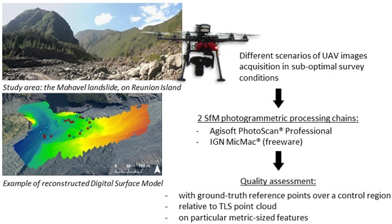
2. Scenario of the Survey and 3D Model Reconstruction

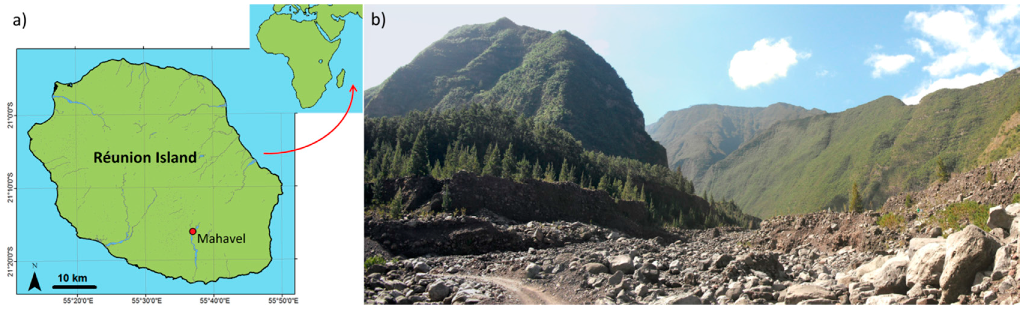
2.1. Description of the Study Area

The study area is located in the upper part of the Rivière des Remparts, a river on the island of La Reunion in the Indian Ocean (Figure 1). This river flows on the Western part of the active volcano of the Piton de la Fournaise. It is approximately 27 km long, up to 500 m wide, with a bed slope of about 5.2%. The upper part of the river, the Mahavel cliff, is an area where huge mass wasting processes have occurred during the last century. The most significant event occurred on 6 May 1965 and the volume of collapsed material reached 50 × 106 m3 [15]. Those mass wasting processes are mainly triggered by intense rainfalls that are common in this tropical area. They can also be influenced by earthquakes linked to the volcanic activity of the Piton de la Fournaise. The transport of the very large quantity of material released in the collapse occurs through bedload transport in the river network, but only during the wet season (November–March), the river bed being dry during most of the year. These particular geomorphological processes create alluvial terraces composed of centimetric to decametric blocks that are, in fact, the bedload transported during the wet season. This variety of boulder sizes is similar in the river bed.
This area was already surveyed as part of a monitoring program of the Réunion landslides [16]. It is barren and has large variety of morphological features covering a range of roughness sizes, such as pebbles of various sizes, eroded terraces and channels. Owing to its wide variety of roughness and terrain, and steep topographic variations (of ±20 m), this area was selected to assess the accuracy of the DSM computed by different SfM photogrammetry software solutions.

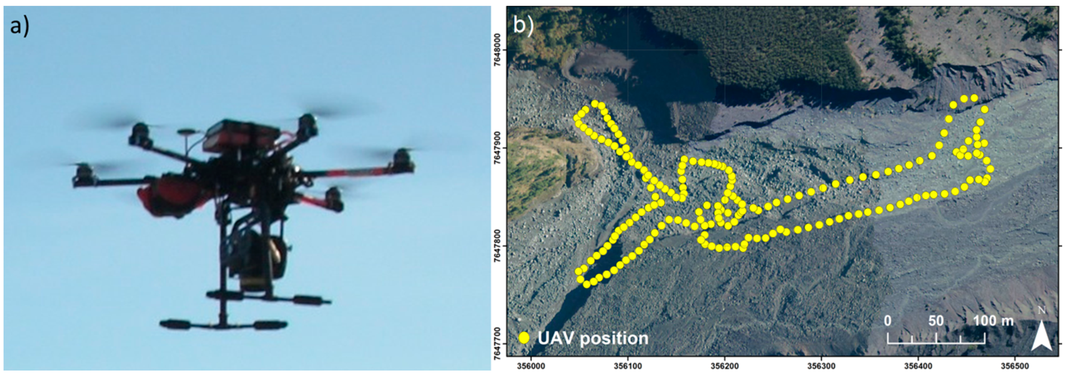
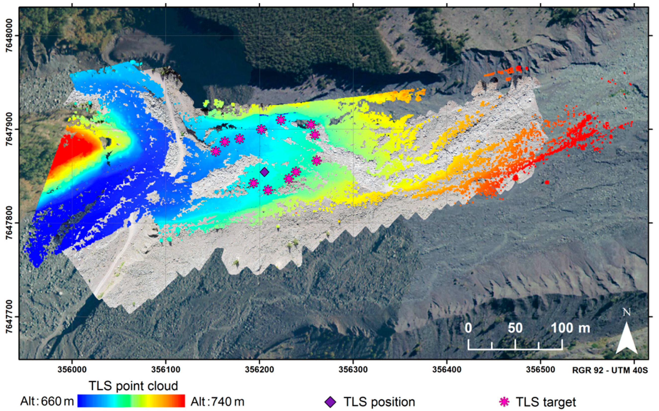
2.2. Data Collection

Data were collected during a UAV flight conducted on 26 May 2015. The survey was performed using DRELIO, an UAV based on a multi-rotor platform DS6, assembled by DroneSys (Figure 2a). This electric hexacopter UAV has a diameter of 0.8 m and is equipped with a collapsible frame allowing the UAV to be folded back for easy transportation. The DS6 weighs less than 4 kg and can handle a payload of 1.6 kg. The flight autonomy of DRELIO is about 20 min. It is equipped for nadir photography with a reflex camera Nikon D700 with a focal length of 35 mm, taking one 12 Mpix photo per second (stored in JPEG fine format). The flight control is run by the DJI® software iOSD. Although DRELIO is able to perform a semi-autonomous flight, take-off and landing, ground station software is used to control the UAV during the flight.
For this study, the flight was performed in “assisted mode”, i.e., without programming the drone, because the number of GPS satellites was not stable and most of the time under the minimum required for automatic mode. The flight altitude was around 100 m, which leads to a spatial resolution of 1.7 cm/pixel. Because of poor GPS reception in this steep-sided environment, the autonomous operation was affected by signal loss. Therefore, ground station software was used in manual mode to monitor the UAV during the flight. For security reasons (e.g., erratic streams of air near the rock faces), the flight plan did not follow the ideal theoretical flight plan. The flight plan is depicted in Figure 2b. During the flight, 278 images were acquired, covering around 7 ha.
Twenty-four highly visible targets were distributed in the study area (Figure 3). These targets are circular disks of 23 cm in diameter, colored in either red or blue. They are georeferenced with post-processed Differential GPS (DGPS), using a Topcon HiPer II GNSS receiver.
The base receiver is placed at a location that has not been previously surveyed. For the duration of the survey (~3 h), this base receiver collects position measurements and saves this data to its internal memory. At the same time, the base station determines differential corrections and transmits them to the RTK (Real Time Kinematic) rover receiver. The RTK rover receiver collects position measurements and accepts corrections from the base station to compute its RTK-corrected position. Each target (GCP, reference points—REF., TLS target) is recorded by the rover as the average position over 10 s (10 epochs) measurements/occupations. After the survey, the Topcon Tools software is used for post-processing the base position. An offset is computed to connect the RTK rover relative measurements to the post-processed absolute base position.
The positioning accuracy depends upon the observed satellite geometry (Geometric Dilution of Precision: GDOP) and the measurement errors. For RTK operations, it is important to consider that the GDOP is dependent on the number of common satellites in view at both the base receiver and the rover receiver. In addition, RTK rover measurements can also be adversely affected by nearby natural or man-made objects that block, interrupt, reflect, or partially obscure satellite signals. The accuracy of the base position, computed at the post-processing step, is 3.1 cm horizontally and 4.5 cm vertically. The precision of the RTK rover relatively to the base position can be up to 1.0 cm horizontally and 1.5 cm vertically [17]. Here, the distance from the base station, not exceeding 100 m, does not really affect the RTK accuracy (impact < 0.1 mm). Averaging the rover position over 10 s also contributes to minimizing the measurement errors. Nevertheless, measurements uncertainties are difficult to estimate. In addition, errors on targets positions may be due to multipath effects (particularly in this mountainous environment). Moreover, as all the targets (GCP, REF. and TLS targets) are measured during the same session, relative to the same base, the accuracy of base position does not impact the comparisons of the different datasets. This is why in the paper we use the precision rather than the accuracy to compare different methods.
The 12 red targets are used as Ground Control Points (GCPs) in the SfM photogrammetry processing chains (PhotoScan® and MicMac®) to compute georeferenced orthophotos and the DSM. The 12 blue targets have been distributed so as to be used as “ground truth” reference points to assess the quality of the results, independently from the photogrammetric software tools. The three blue targets (REF.10, REF.11, REF.12) situated in the Western part of the area appear to be affected by significant GPS positioning errors, probably due to multi-path reflections on the nearby steep face. Therefore, these targets will not be taken into account in the following calculations, leaving nine targets for “ground truth” reference points.
As the study area is very rugged, placing GCPs and reference targets and measuring their position is a very time-consuming step of the survey. Some parts of the area are impracticable because of obstacles. As a consequence, targets were not set up all over the study area. Moreover, in such environments, it may be difficult for people who set up the targets to have a synoptic view of their distribution. Considering the imperfect distribution of the GCPs, the study area can be subdivided into areas within the control region and areas outside. Such a configuration is not uncommon when using UAVs, as they constitute a solution for surveying areas that are not easily accessible.
To complement these datasets, a high resolution Terrestrial Laser Scanner (TLS) survey was simultaneously carried out using a Riegl© VZ-400 TLS. The TLS point cloud was collected with an angular resolution of 0.04° (vertically and horizontally) from one station. More than 10.6 million points were recorded over the study area (Figure 4); however, the point cloud density is heterogeneous. The TLS dataset was georeferenced indirectly, using 12 reflective targets. The absolute position of these targets was measured by post-processed RTK GPS, while their relative position in the point cloud was obtained with the TLS by semi-automatic detection and re-scanning at very fine spatial resolution. A least squares algorithm was applied to compute the transformation providing the best fit between absolute and relative positions of the targets. The residual error of this georeferencing process is about 5 cm for the targets. Such uncertainties result in errors up to 32 cm at a range of 300 m from the TLS position (e.g., in the Eastern part of the point cloud).
The whole survey, with two teams working in parallel, took more than 3 h.

3. Photogrammetric Processing Chain

3.1. PhotoScan Overview

PhotoScan Professional (version 1.1.5) is a commercial product developed by AgiSoft®. This software is commonly used for archeological purposes [18,19], but also for topography and mapping [20]. The procedure for deriving orthophotographs and the DSM consists of four main stages. There are a number of parameters to adjust at each of these steps:
  • Camera alignment by bundle adjustment. Common tie points are detected and matched on photographs so as to compute the external camera orientation parameters for each picture. Camera calibration parameters are refined, simulating the distortion of the lens with Brown’s distortion model [21]. This model allows correcting both for radial and tangential distortions. The “High” accuracy parameter is selected (the software works with original size photos) to obtain more accurate camera position estimates. The number of matching points (tie points) for every image can be limited to optimize performance. The default value of this parameter (1000) is kept.
  • Creation of the dense point cloud using the estimated camera positions and the pictures themselves. PhotoScan calculates depth maps for each image. The quality of the reconstruction is set to “High” to obtain a more detailed and accurate geometry.
  • Reconstruction of a 3D polygonal mesh representing the object surface based on the dense point cloud. The surface type may be selected as “Arbitrary” (no assumptions are made on the type of the reconstructed object) or “Height field” (2.5D reconstruction of planar surfaces). Considering the complexity of the study area (blocks, terrace fronts), the surface type is set to “Arbitrary” for 3D mesh construction, even if this implies higher memory consumption and higher processing time. The user can also specify the maximum number of polygons in the final mesh. In our study, this parameter is set to “High” (i.e., 1/5 of the number of points in the previously generated dense point cloud) to optimize the level of detail of the mesh.
  • The reconstructed mesh can be textured following different mapping modes. In this study, we used the default “Generic” mode.
The intermediate results can be checked and saved at every step. At the end of the process, a DSM and an orthophotograph are exported in GeoTiff format, without any additional post-processing (optimization, filtering, etc.). This format implies that datasets are converted to 2.5D. Such a conversion may have an effect on the reconstruction of complex structures. However, as there are almost no overhanging elements in the study area, the impact of the 2.5D conversion remains limited and is therefore neglected in this study, considering that photos are acquired from a nadir point of view and that both PhotoScan and MicMac DSM are affected in the same way by this conversion.
The software is user-friendly, but the adjustment of parameters is limited by pre-defined values. It can be noted that the user manual describes mainly the general workflow and gives only very limited details regarding the theoretical basis of the underlying calculations and the associated parameters.

3.2. MicMac Overview

MicMac (acronym for “Multi-Images Correspondances, Méthodes Automatiques de Corrélation”) is an open-source photogrammetric software suite developed by IGN® for computing 3D models from sets of images [22,23]. Micmac® chain is very open and most of the parameters can be finely tuned. In this study, we use the version v.5348 for Linux.
The standard “pipeline” for transforming a set of aerial images in a 3D model and generating an orthophoto with MicMac consists of four steps.
  • Tie point computation: the Pastis tool uses the SIFT++ algorithm [24] for the tie point pair generation. This algorithm creates an invariant descriptor that can be used to identify the points of interest and match them even under a variety of perturbing conditions such as scale changes, rotation, changes in illumination, viewpoints or image noise. Here, we used Tapioca, the simplified tool interface, since the features available using Tapioca are sufficient for the purpose of our comparative study. Also note that the images have been shrunk to a scaling of 0.25.
  • External orientation and intrinsic calibration: the Apero tool generates external and internal orientations of the camera. The relative orientations were computed with the Tapas tool in two steps: first on a small set of images and then by using the calibration obtained as an initial value for the global orientation of all images. The distortion model used in this module is a Fraser’s radial model with decentric and affine parameters and 12 degrees of freedom. Recently, Tournadre et al. (2015) published a study [25] presenting the last evolutions of MicMac’s bundle adjustment and some additional camera distortion models specifically designed to address issues arising with UAV linear photogrammetry. Indeed, UAV surveys along a linear trajectory may be problematic for 3D reconstruction, as they tend to induce “bowl effects” [25,26] due to a poor estimation of the camera’s internal parameters. This study therefore puts to the test the refined radial distortion model “Four 15 × 2” [23,25] for camera distortion. Using GCPs, the image relative orientations are transformed with “GCP Bascule” into an absolute orientation within the local coordinate system. Finally the Campari command is used to compensate for heterogeneous measurements (tie points and GCPs).
  • Matching: from the resulting oriented images, MicMac computes 3D models and orthorectification. The calculation is performed iteratively on sub-sampled images at decreasing resolutions, the result obtained at a given resolution being used to predict the next step solution. The correlation window size is 3 × 3 pixels.
  • Orthophoto generation: the tool used to generate orthomosaics is Tawny. It is an interface to the Porto tool. Tawny merges individual rectified images that have been generated by MicMac in a global orthophoto and optionally does some radiometric equalization.
At each step, with MicMac the user can choose any numerical value, whereas PhotoScan only offers preset values (“low”, “medium” and “high”). As for PhotoScan, the intermediate results can be checked and saved at every step. At the end of the process, a DSM and an orthophotograph are exported in GeoTiff format, without any additional post-processing.
For both software packages, the processing time depends on the RAM capacity of the computer, memory requirements increasing with the size and number of images and with the desired resolution.

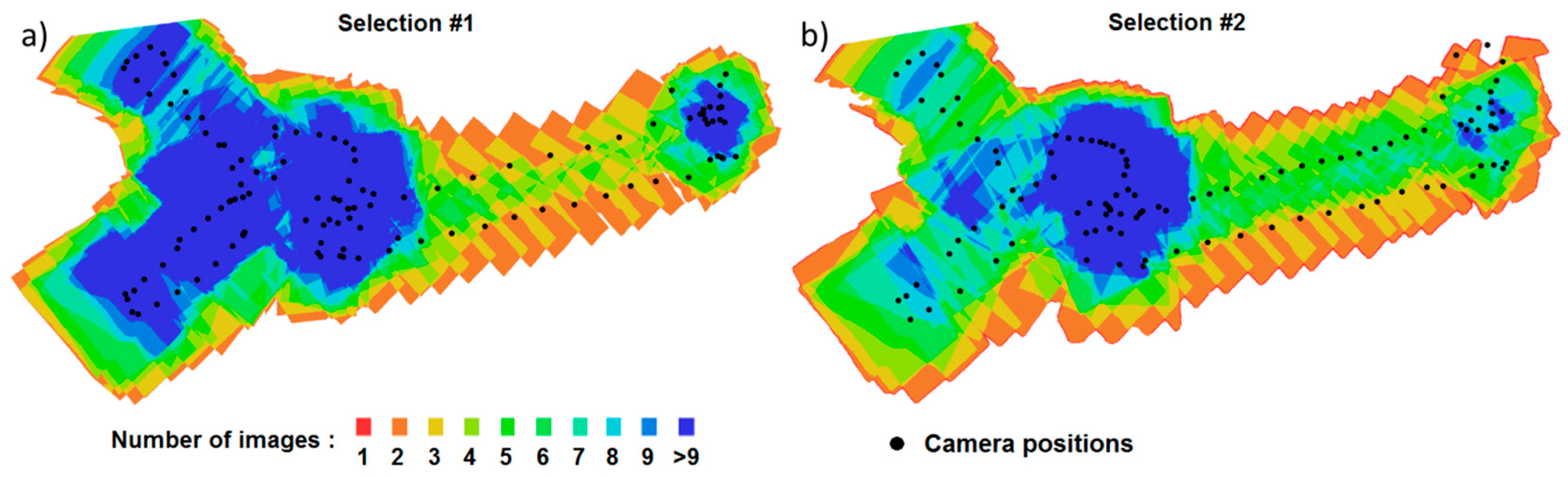
3.3. Images Selection
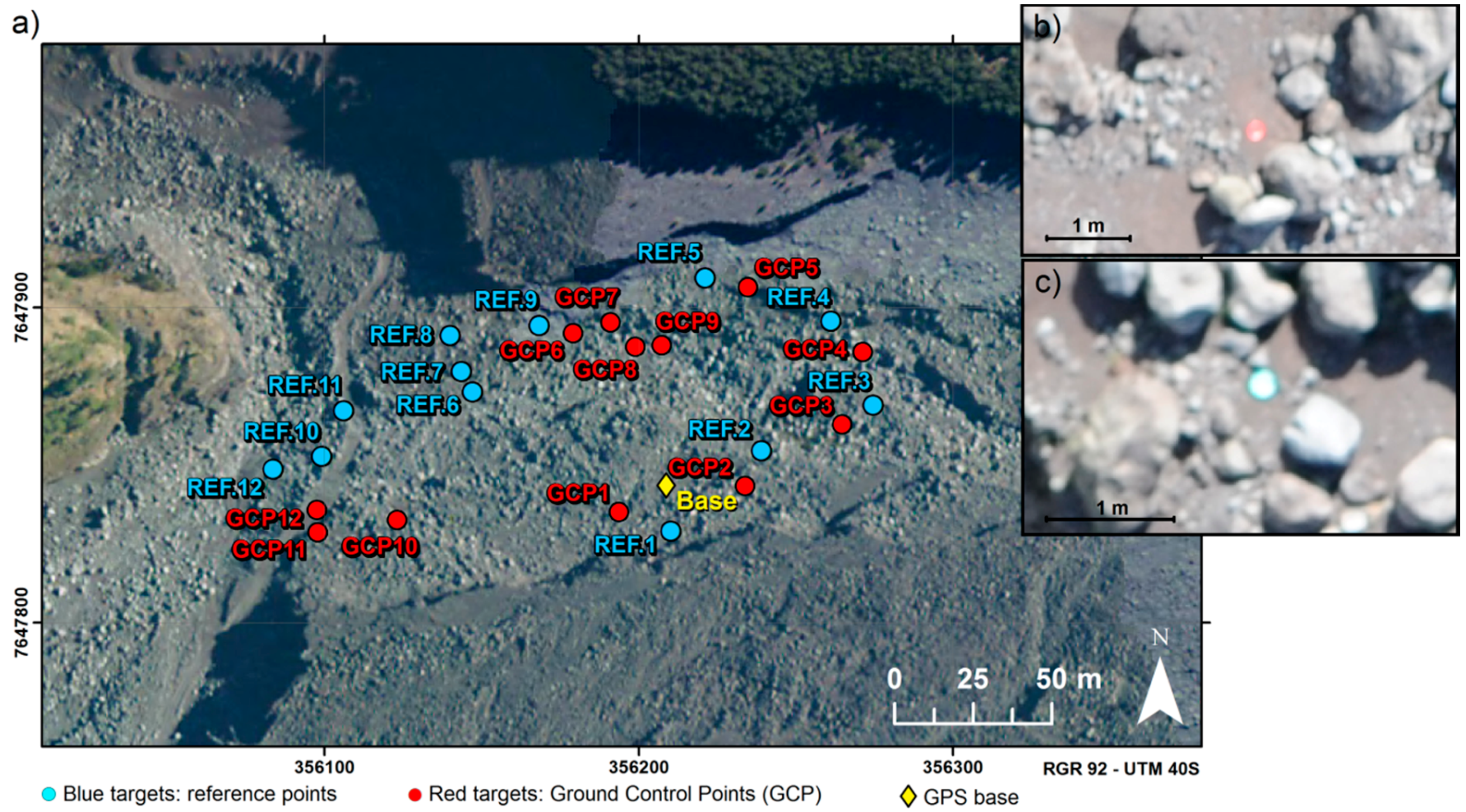
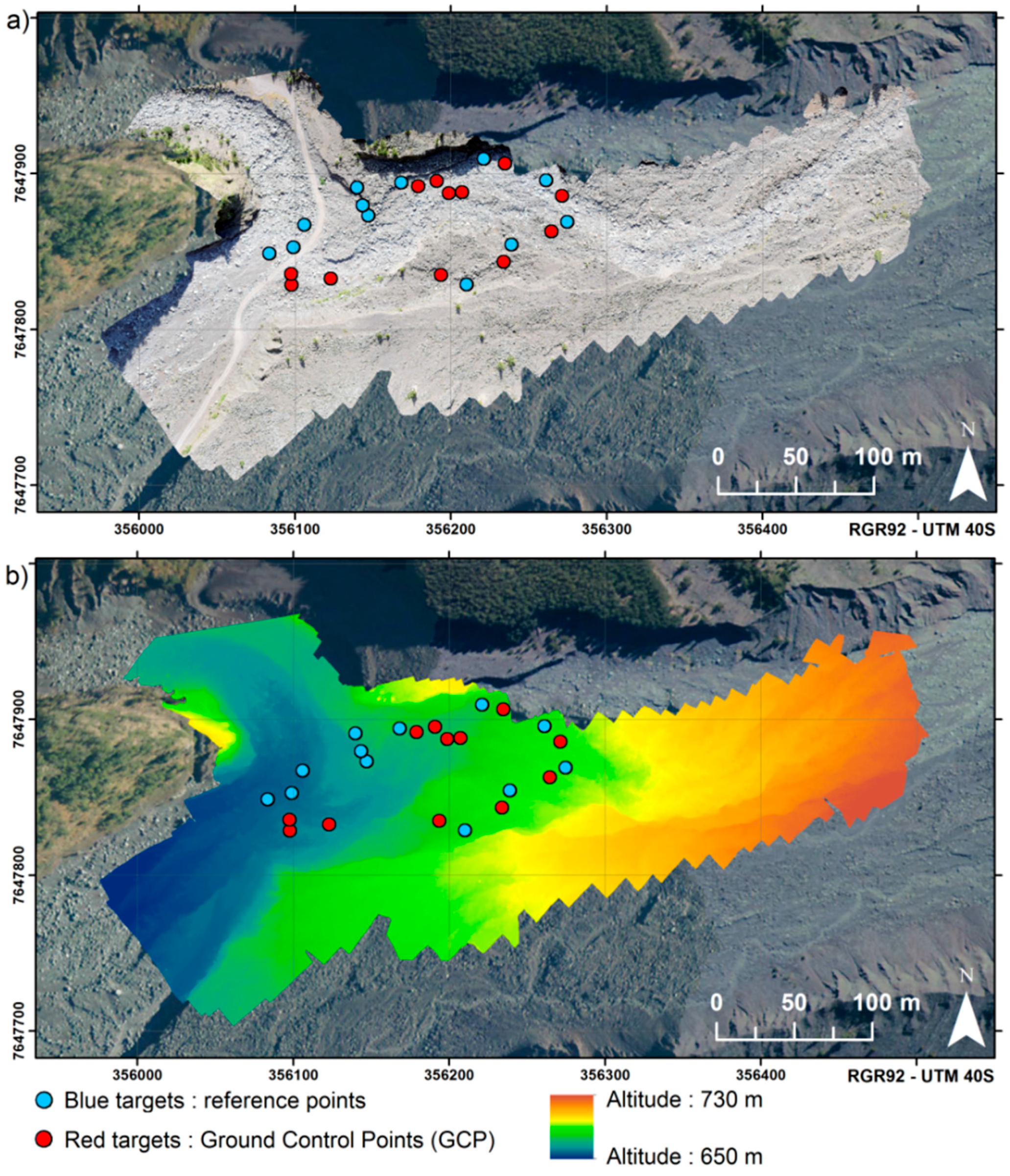
Some unusable images (e.g., images taken during take-off and landing, blurred images, etc.) were discarded from the original set of photographs. From the remaining photographs, two sets of images were created. The first one is generated automatically, selecting every image acquired when the drone was at an elevation close to 100 m. This set is composed of 121 photographs. The second selection is carried out manually, selecting images offering a good compromise to cover the area of interest, to have sufficient overlap and to avoid redundancy. As the area situated between GCP 4 and GCP 6 (Figure 3) is the most interesting to monitor Mahavel landslide, more photographs are selected in this area. The second set of images counts 109 images.
Manually selecting photos allows reducing the number of images, avoiding redundancy and speeding-up the process. The image selection step may appear tedious, but it may significantly reduce the processing time and the GCP tagging step. The overlap between images for each selection is depicted in Figure 5. Both mapped areas are very similar. There are fewer images in the manual selection (Selection #2), but they are more homogeneously distributed.

3.4. GCPs Tagging

GCPs are essential to achieve results of the highest quality, both in terms of geometrical precision and georeferencing accuracy. Great care is given to tag the GCPs (for each GCP, the photo is zoomed sufficiently so that the operator can precisely place the markers). Both PhotoScan and MicMac offer a guided marker placement option, which significantly speeds up the GCPs’ tagging process. This option implies that GCPs tagging is done after the photo alignment step. In the guided approach, once a GCP has been marked on at least two photos, the projection of its position on other photos is automatically indicated. This position can then be refined manually. Nevertheless, the step of GCPs tagging remains time-consuming for the operator (more than 1 h to tag the GCPs on all the photos of Selection #2 in the present study).
In order to evaluate the uncertainty due to the operator-dependent tagging step, tests were conducted on a set of 25 targets to compare GCPs tagging accuracy between two operators. The mean deviation between the positions pointed by operators is of 0.3 pixel. In addition, another test was carried out where an operator twice pointed (in two independent sessions) to all the GCPs on all the photos of Selection #2 (132 tagged GCPs). The mean deviation between the positions pointed to during both sessions is of 0.4 pixel. The impacts on the resulting DSM are negligible (less than 1 cm).

3.5. Processing Scenarios

Surface reconstruction is performed on the one hand using PhotoScan, and using MicMac on the other. Both SfM photogrammetric processes are computed with the same set of images and the same set of GCPs. GCPs are manually tagged on the images.
Four scenarios are tested:
  • Scenario 1: the process is performed with the automatic selection of 121 photographs (Selection #1), using full-resolution images, i.e., 4256 × 2832 pixels (12 Mpix), and 12 GCPs.
  • Scenario 2: the process is performed with the manual selection of 109 photographs (Selection #2), using full-resolution images and 12 GCPs.
  • Scenario 3: the process is performed with the set of 109 selected photographs, using reduced-quality images, i.e., 2128 × 1416 pixels (3 Mpix), and 12 GCPs. The images of the datasets were down-sampled from 12 Megapixels (Mpix) to 3 Mpix, selecting one line and one sample out of two without modifying the color content of the pixels (nearest-neighbor approach).
  • Scenario 4: the process is performed with the set of 109 selected photographs using full-resolution images and only six GCPs: GCP 1, GCP 2, GCP 6, GCP 7, GCP 8 and GCP 9. The goal of this scenario is to test the impact of the number of GCPs and their distribution within the control region. Only the GCPs of the central part of the control region are therefore considered in order to assess in this case the errors on the external parts of the area [9]. The results of this scenario would be affected both by reducing the number of GCPs and by changing their distribution.
For each test, a DSM (spatial resolution of 4 cm) and an orthophotograph (spatial resolution of 2 cm) are generated (Figure 6). They are integrated in a GIS environment in ArcGIS© software, for evaluation purposes.

4. Results and Discussion

4.1. Effects of the Refined Distortion Model on MicMac Processing Chain

Outside of the control region, the images are acquired on two quasi-parallel lines of flight. Linear sequences of images have been shown to yield warped 3D models due to a drift in bundle adjustment [25,26].
Before processing data with MicMac based on the different scenarios, the MicMac module for UAV linear photogrammetry [25] has been put to the test. These additional distortion models integrated into MicMac have been developed for long linear surveys, especially for riverbed monitoring over several kilometers. Even if the study area is more “compact” here, the refined distortion models are tested to find out whether, in our case, they improve the accuracy of the solution. Scenario 1 has been implemented on one hand with a basic radial distortion model (Fraser’s radial model) and, on the other hand, with a refined radial distortion model (Four 15 × 2) with a polynomial correction of degree 7, referred in the following as “MicMac-rdm”. The accuracy of the resulting reconstructions is assessed using eight reference targets (Table 1).
With MicMac, the vertical Root Mean Square Error (RMSE) is 8.0 cm, while it is 60% lower with Micmac-rdm.
As the targets are not covering the entire surveyed area, further comparisons are carried out to assess the uncertainty of the reconstructed DSM outside of the control region. A Digital Elevation Model (DEM) of Difference between MicMac-rdm and MicMac is computed (Figure 7a) and altitude profiles are extracted (Figure 7b). The profile extracted from TLS data can be used as a reference, although (i) it is fragmented because of no-data zones induced by occlusions and (ii) the TLS dataset is also subject to greater uncertainty outside of the control region. The profile extracted from the PhotoScan DSM is also displayed for relative comparisons. It appears that the MicMac-rdm DSM and the MicMac DSM are nearly similar over the control region (Figure 7a) where the GCPs are located. In contrast, in the external part of the area, the MicMac-rdm DSM shows higher mean elevations than the MicMac DSM, which is affected by bowl effects. The refined distortion model increases the altitude of the external parts of the DEM up to 50 cm in the Western part of the study area, and up to 3 m in the Eastern part. The altitude profiles (Figure 7b) highlight that the stereophotogrammetric DSMs are below TLS data. MicMac-rdm appears more efficient than MicMac with basic distortion model since the altitude profile derived from the DSM computed using MicMac-rdm is very similar to the PhotoScan profile and closer to TLS data than the profile obtained from MicMac. It can be noted that PhotoScan gives results closer to the TLS dataset outside of the control region. Brown’s distortion model implemented in PhotoScan therefore seems more adapted than the refined distortion model implemented in MicMac-rdm. In the following, MicMac-rdm will be used when running MicMac tests.

4.2. Quality Assessment of PhotoScan and MicMac within the Control Region Using Ground-Truth Reference Points

For each scenario, the horizontal Root Mean Square Error (RMSE) is calculated from the differences between the xy positions of the nine “ground-truth” reference points (the blue reference targets) measured by RTK DGPS and their xy positions pointed out on the georeferenced PhotoScan/MicMac orthophoto. The vertical RMSE is calculated from the differences between the z positions of the blue targets measured by RTK DGPS and their altitude on the PhotoScan/MicMac reconstructed DSM. These errors are thus computed independently of the estimation made by both software packages. The results are presented in Table 2.
In scenario 1, the horizontal RMSE is 4.5 cm with PhotoScan and 3.5 cm with Micmac; the vertical RMSE are 3.9 cm and 3.2 cm, respectively. These RMSEs are of the same order of precision as the uncertainty on post-processed DGPS measurements. Expressing these results as a ratio against the mean flying height (100 m here), the vertical RMSE obtained with PhotoScan and MicMac are respectively of 39 cm/km and 32 cm/km. The results are very satisfying, since Vallet et al. in [27] report a 10–15 cm accuracy when flying at 150 m (i.e., 66.7–100 cm/km) and [13] achieve a 2.5–4 cm accuracy when flying at only 40–50 m (i.e., 50–80 cm/km).
In scenario 2, the vertical RMSE is higher (12.4 cm) than in scenario 1 for PhotoScan. With MicMac, the vertical RMSE (4.7 cm) is lower than with PhotoScan. The reason for the difference between PhotoScan and MicMac vertical RMSE is not clear. On the reference target REF.8, the error on MicMac DEM is 7.8 cm, whereas it is 25.1 cm on PhotoScan DEM. One hypothesis is that this difference may be due to a localized artefact around that reference target. James and Robson suggest in [9] that the SIFT algorithm can sometimes produce relatively poor feature-position precision, which is maybe the case here.
In scenario 3, the processing time is consequently reduced, however, as the number of pixels has been reduced, it is more difficult for the user to accurately tag the GCPs. Moreover, the resolution of the resulting orthophoto and DSM is twice lower than the resolution with images at full resolution. For PhotoScan, the horizontal and vertical RMSE are respectively of 5.8 cm and 15.0 cm, whereas they are respectively of 3.2 cm and 6.3 cm for Micmac. Nevertheless, to be comparable to the results of scenario 2, these values have to be reported relatively to the resolution. For this reason, the values are also given in pixels into brackets (with a pixel of 1.7 cm for scenario 2, and 3.4 cm for scenario 3).
In scenario 4, only six GCP are used in the processing chain: GCP 1, GCP 2, and GCP 6 to GCP 9. The horizontal RMSE (4.4 cm for PhotoScan and 4.7 cm for MicMac) is a bit higher than with 12 GCPs (scenario 2). The vertical RMSE is of 7.3 cm with PhotoScan (against 12.4 cm for scenario 2). It suggests that some of the unused GCPs (GCP 3, 4, 5, 10, 11 or 12) may have been a source of error in scenario 2, likely because of bad positioning. With MicMac, the vertical RMSE of scenario 4 (4.8 cm) is nearly similar to scenario 2. The number and repartition of GCPs seem to have a low impact on the DSM and orthophotograph’s accuracy at the scale of the control region.

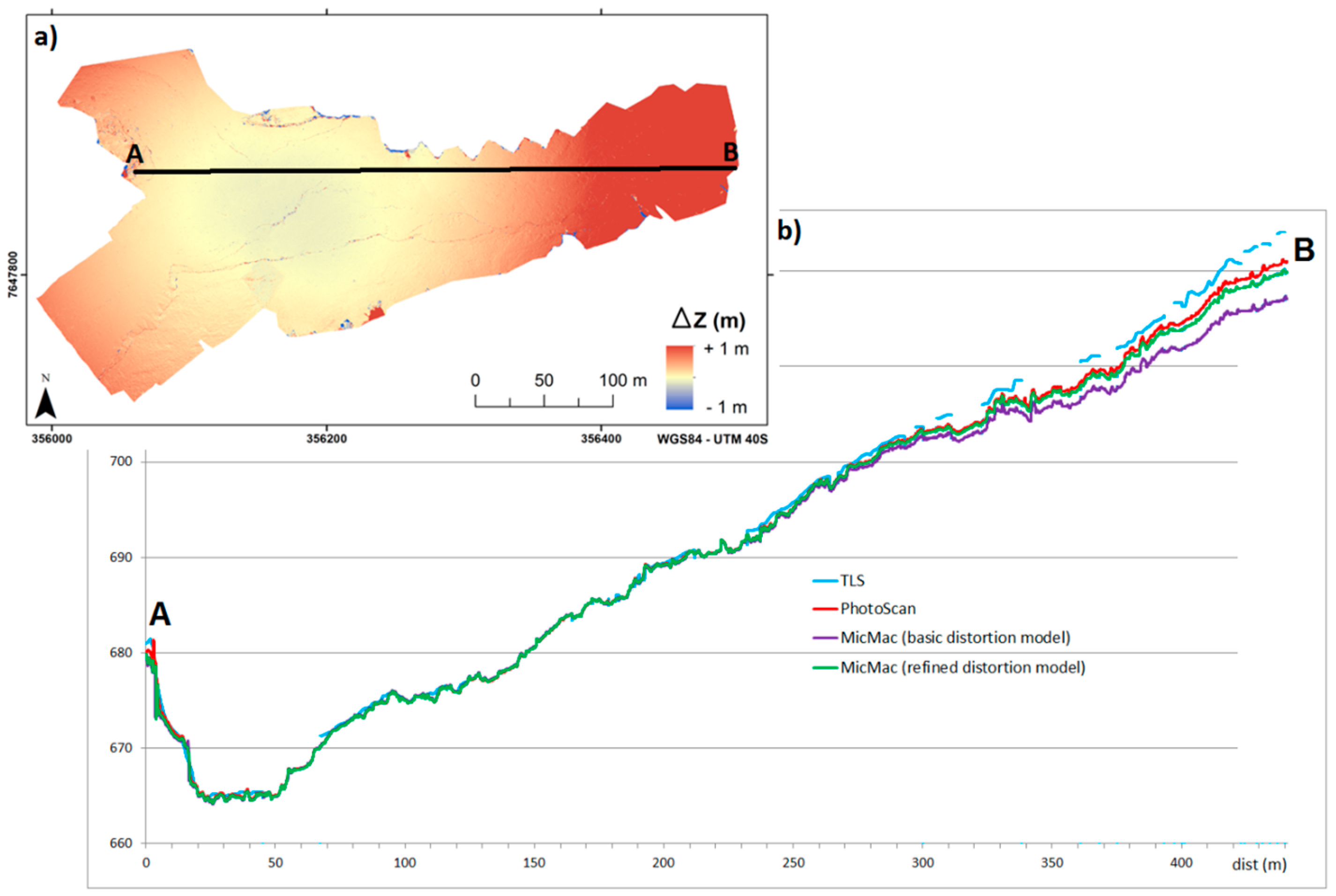
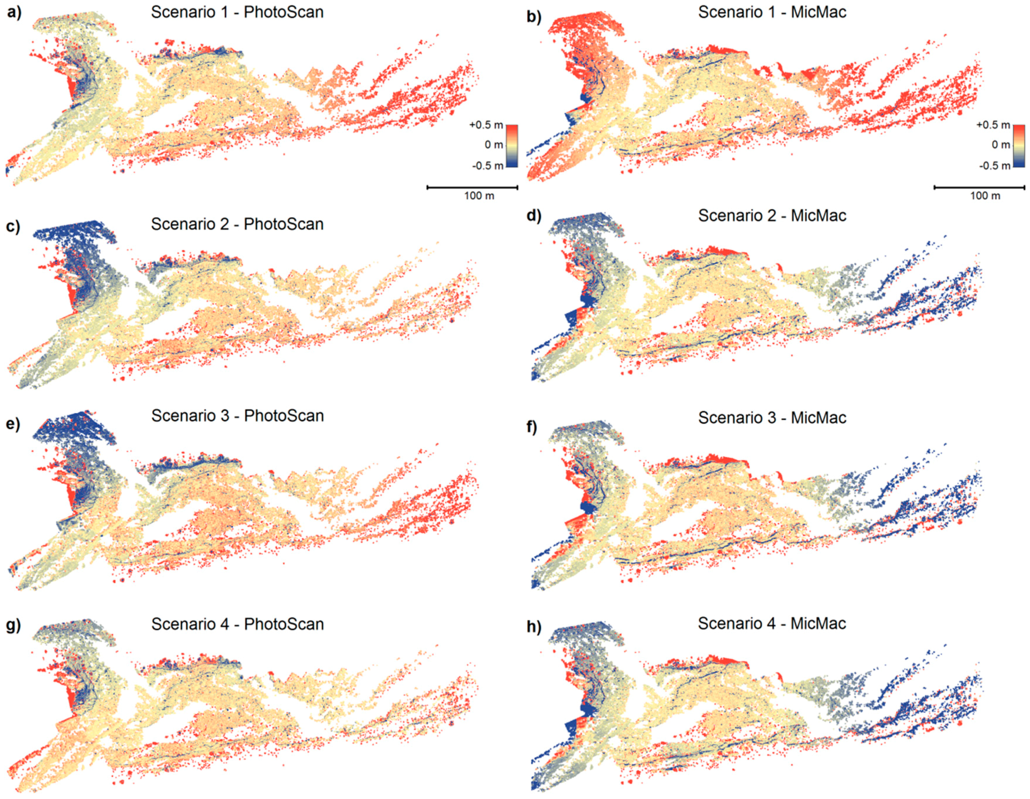
4.3. Relative Quality Assessment of PhotoScan and MicMac with Respect to the TLS Point Cloud over the Whole Study Area

At the same time as the UAV survey, the 3D positions of 10.6 million points were measured by TLS. As the TLS point cloud is acquired from a terrestrial point of view, the point cloud is very dense on the vertical scanned surfaces. However, because of the complex topography causing occlusion effects, the TLS point cloud presents some areas without data. As expected, given the poor GPS reception typical in a mountainous context, the accuracy of the TLS dataset is low. The TLS dataset is also subject to greater uncertainties outside of the control region. Nevertheless, it can be used as a point of comparison to analyze in which way the results of the photogrammetric chains drift where there is no GCP. Thus, the TLS dataset serves as a reference DTM, but it is not considered as ground truth.
To avoid interpolations effects from meshing the sparse TLS point cloud, this dataset is kept in XYZ point cloud format. Both PhotoScan and MicMac DSMs are thus directly compared to the georeferenced TLS point cloud, using the FlederMaus® CrossCheck tool. For each point of the TLS point cloud, ZTLS is compared to the z value of the corresponding xy-coordinates cell in the photogrammetric DSM raster. The results of the comparison (ZTLS-DSM) are presented in Figure 8 and Table 3. In Figure 8, the light yellow areas depict areas where the altitude of TLS point cloud is equal or close to the altitude of the DSM computed by SfM photogrammetry. In red areas, the TLS point cloud is above the photogrammetric DSM. Conversely, in blue areas, the photogrammetric DSM is above the TLS point cloud.
It may be noted that, in the Eastern part of the study area, the MicMac DSM has lower elevation than the TLS point cloud for scenario 1, whereas it has higher elevation than the TLS point cloud for other scenarios. Tournadre et al. [25] mention that a high number of images ensuring an extensive overlap is favorable for UAV linear surveys. In this study, the number of images affects the result of the refined distortion model in MicMac: with the Selection #1 of 121 images, the bowl effect is downward, whereas it is upward with the Selection #2 of 109 images.
Considering the RMS errors obtained for both photogrammetric DSMs within the control region (Table 2) and the georeferencing error against the TLS point cloud, the results are satisfying, since mean differences lower than 10 cm (Table 3) are achieved. Since the point density of the TLS point cloud significantly decreases with increasing distance from the TLS position, the control region, which represents 36% of the scanned surface, contains 97% of the point cloud. Since the comparison gives the same weight to each point of the TLS cloud, the results of the DSMs to TLS comparison in Table 3 are mainly representative of the comparison in the control region where most of the points from the TLS cloud are located. To complement Table 3, Figure 8 depicts the spatial distribution of the error. As expected, the offsets between the photogrammetric DSMs and the TLS point cloud are low within the control region. Deviations appear outside of the control region, growing with distance to the control region, confirming that the number of GCPs and their distribution are key parameters for linear surveys [26,28]. In the Eastern part of the study site, PhotoScan seems to provide better results than MicMac because of milder “bowl effects”. This suggests that the Brown’s distortion model implemented in PhotoScan is more relevant in this context than the refined radial model implemented in MicMac.
It appears that the mean differences to the TLS DSM are higher with MicMac than with PhotoScan (Table 3). With MicMac, the errors assessed by comparison to the TLS point cloud (Table 3) are also higher than the errors assessed using ground truth reference points (Table 2). Such an increase in the error may be partly due to greater uncertainties on TLS dataset than on the ground truth reference points, as well as discrepancies on the reconstruction of sharp-relief zones. Indeed, the gaps on the southern and northern edges of the TLS point cloud coincide with the terraces fronts (Figure 4), which are challenging to compute by aerial photogrammetry. Moreover, such poor reconstructions largely contribute to increasing the error. Indeed, first, a horizontal shift of some centimeters in such complex environments may generate important vertical offsets in DSM differencing, implying errors in volume budgets. Second, as the sections of the TLS point cloud corresponding to quasi-vertical terraces fronts are generally very dense, the relative weight of these areas in the error calculation is very large.

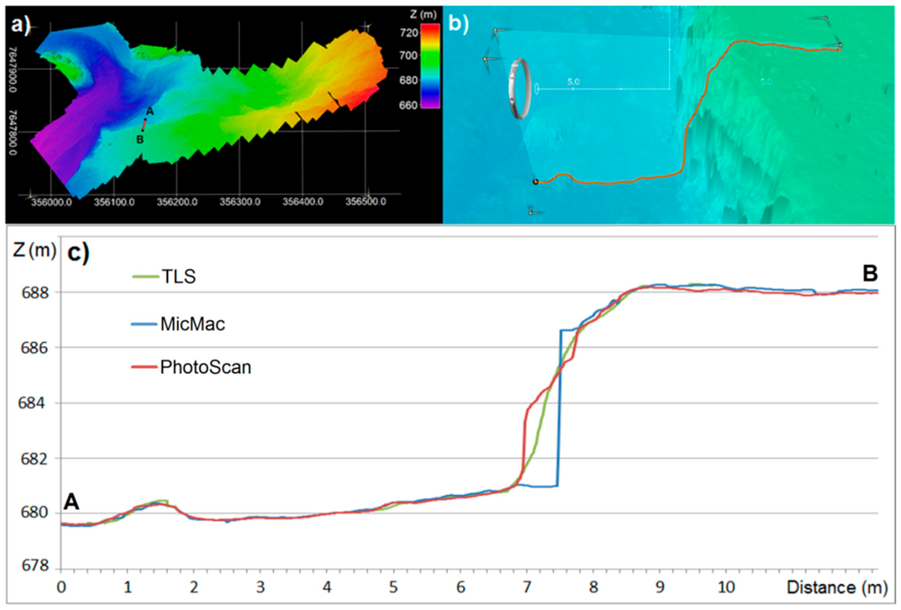
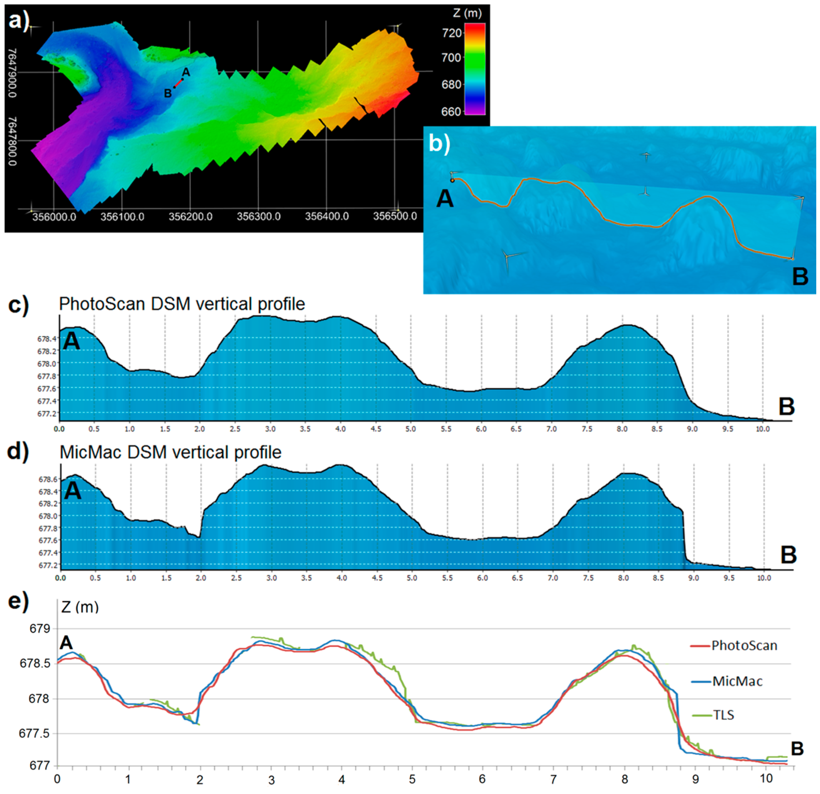
4.4. Quality Assessment of PhotoScan and MicMac on Particular Metric Features

As a “1st order” interpretation, spatial low-frequency components describe moderate changes in the relief, such as the average slope, while spatial high-frequency components depict local structure or details. In the previous paragraph, the quality of the DSM was assessed on low-frequency components. The aim of this section is to compare the ability of each method to reconstruct details in topography.
A 12 m-long vertical profile over a terrace front has been extracted from PhotoScan DSM, MicMac DSM and TLS point cloud. The results are presented in Figure 9. The RMS offset between the profiles extracted from both DSMs is 71 cm (Table 4). Comparing these profiles with the TLS point cloud, it can be noted that PhotoScan gives better results, particularly on the terrace front where Micmac’s reconstruction is very steep. Using oblique imagery may limit such artefacts; nevertheless, it would increase occlusions and shadowing.
With MicMac, sharp relief variations also appear on the 10 m-long vertical profile extracted along a set of rocky blocks (Figure 10). The surface reconstructed with PhotoScan is smoother. However, the Root Mean Square (RMS) offset between both photogrammetric DSMs is only 6 cm, and 17 cm with the TLS dataset.
Even if these offsets due to spatial high-frequencies reconstruction remain low at the scale of the topographic variations, they may have an impact on sediment budgets in diachronic DSM differencing [29,30]. In such complex environments, a horizontal shift of a few centimeters may create large shifts in the vertical direction due to highly sloping surfaces. These offsets partly explain the differences previously observed in the comparisons with the TLS point cloud (Figure 8).

5. Conclusions

This study aims at comparing the reconstruction of the DSM and orthophotograph obtained with two software packages for SfM photogrammetry. AgiSoft® PhotoScan Pro, a commercial solution, and MicMac, an open-source solution proposed by IGN©, are tested with UAV images collected in challenging conditions. The sensitivity of each software tool to different parameters (images selection, images resolution, position and number of GCPs) has been analyzed. The MicMac-rdm package recently developed for linear surveys greatly improves the quality of the results compared to the basic distortion model. Nevertheless, Brown’s distortion model implemented in PhotoScan still seems more appropriate than the refined radial model implemented in MicMac in this particular context of rugged terrain.
The results are analyzed in two ways: (i) using ground truth reference targets (distinct from the GCPs, but located in the same area) within the control region; and (ii) by comparison with a TLS point cloud (at the scale of the entire surveyed area). To limit the impact of GPS uncertainties in the comparison, we consider precision rather than accuracy. Within the control region, both software packages provide satisfying results, with an achievable precision of 3–4 cm. Outside of the control region, the comparison with TLS dataset shows that both reconstructed DSMs tend to deviate in the Eastern part because of “bowl’s effects” in the absence of GCPs. Nevertheless, PhotoScan seems to provide better results than MicMac thanks to a more relevant distortion model (limiting deviations in the DSM) and a better reconstruction of the terrace front.
Despite the bias on the reconstruction outside of the control region, which has an impact on comparisons, the DSM and orthophotograph may be useful in other respects. Indeed, the reconstruction remains consistent and can therefore be useful to address a number of topics such as the raw estimation of the topography, the study of ground coverage or granulometry estimation.

Acknowledgments

This work is financially supported by the EU through the FP7 project IQmulus (FP7-ICT-2011-318787).

Author Contributions

Marion Jaud and Sophie Passot conceived and designed the experiments and analyzed the data; Marion Jaud, Réjanne Le Bivic and Philippe Grandjean performed the surveys; Réjanne Le Bivic, Nicolas Le Dantec and Christophe Delacourt contributed to data analysis and supervised the writing of the manuscript; Marion Jaud wrote the paper.

Conflicts of Interest

The authors declare no conflict of interest.

References

  1. Delacourt, C.; Allemand, P.; Jaud, M.; Grandjean, P.; Deschamps, A.; Ammann, J.; Cuq, V.; Suanez, S. DRELIO: An unmanned helicopter for imaging coastal areas. J. Coast. Res. 2009. [Google Scholar] [CrossRef]
  2. Mancini, F.; Dubbini, M.; Gattelli, M.; Stecchi, F.; Fabbri, S.; Gabbianelli, G. Using unmanned aerial vehicles (UAV) for high-resolution reconstruction of topography: The structure from motion approach on coastal environments. Remote Sens. 2013. [Google Scholar] [CrossRef] [Green Version]
  3. Honkavaara, E.; Saari, H.; Kaivosoja, J.; Pölönen, I.; Hakala, T.; Litkey, P.; Mäkynen, J.; Pesonen, L. Processing and assessment of spectrometric, stereoscopic imagery collected using a lightweight UAV spectral camera for precision agriculture. Remote Sens. 2013. [Google Scholar] [CrossRef] [Green Version]
  4. Henry, J.-B.; Malet, J.-P.; Maquaire, O.; Grussenmeyer, P. The use of small-format and low-altitude aerial photos for the realization of high-resolution DEMs in mountainous areas: Application to the super-sauze earthflow (Alpes-de-Haute-Provence, France). Earth Surf. Proc. Landf. 2002, 27, 1339–1350. [Google Scholar] [CrossRef] [Green Version]
  5. Fonstad, M.A.; Dietrich, J.T.; Courville, B.C.; Jensen, J.L.; Carbonneau, P.E. Topographic structure from motion: A new development in photogrammetric measurement. Earth Surf. Proc. Landf. 2013, 38, 421–430. [Google Scholar] [CrossRef]
  6. Westoby, M.J.; Brasington, J.; Glasser, N.F.; Hambrey, M.J.; Reynolds, J.M. “Structure-from-motion” photogrammetry: A low-cost, effective tool for geoscience applications. Geomorphology 2012, 179, 300–314. [Google Scholar] [CrossRef] [Green Version]
  7. Woodget, A.S.; Carbonneau, P.E.; Visser, F.; Maddock, I.P. Quantifying submerged fluvial topography using hyperspatial resolution UAS imagery and structure from motion photogrammetry. Earth Surf. Proc. Landf. 2015, 40, 47–64. [Google Scholar] [CrossRef]
  8. Lowe, D.G. Object recognition from local scale-invariant features. In Proceedings of the 7th IEEE International Conference on Computer Vision (ICCV), Kerkyra, Corfu, Greece, 20–25 September 1999; pp. 1150–1157.
  9. James, M.R.; Robson, S. Straightforward reconstruction of 3D surfaces and topography with a camera: Accuracy and geoscience application. J. Geophys. Res. 2012. [Google Scholar] [CrossRef]
  10. Colomina, I.; Molina, P. Unmanned aerial systems for photogrammetry and remote sensing: A review. ISPRS J. Photogramm. Remote Sens. 2014, 92, 79–97. [Google Scholar] [CrossRef]
  11. Neitzel, F.; Klonowski, J. Mobile 3D mapping with a low-cost UAV system. Int. Arch. Photogramm. Remote Sens. Spat. Inf. Sci. 2011, 38, 39–44. [Google Scholar] [CrossRef]
  12. Küng, O.; Strecha, C.; Beyeler, A.; Zufferey, J.-C.; Floreano, D.; Fua, P.; Gervaix, F. The accuracy of automatic photogrammetric techniques on ultra-light UAV imagery. Int. Arch. Photogramm. Remote Sens. Spat. Inf. Sci. 2011, 38, 125–130. [Google Scholar] [CrossRef]
  13. Harwin, S.; Lucieer, A. Assessing the accuracy of georeferenced point clouds produced via multi-view stereopsis from unmanned aerial vehicle (UAV) imagery. Remote Sens. 2012, 4, 1573–1599. [Google Scholar] [CrossRef]
  14. Anders, N.; Masselink, R.; Keegstra, S.; Suomalainen, J. High-res digital surface modeling using fixed-wing UAV-based photogrammetry. In Proceedings of the Geomorphometry, Nanjing, China, 16–20 October 2013.
  15. BRGM. Etude Géologique de L’éperon Rive Droite de la Rivière des Remparts Situé au Droit du Barrage de Mahavel. Evolution de la Morphologie du Barrage Après le Passage du Cyclone “Denise”; Technical Report TAN 66-A/12; BRGM: Orléans, France, 1966. [Google Scholar]
  16. Le Bivic, R.; Delacourt, C.; Allemand, P.; Stumpf, A.; Quiquerez, A.; Michon, L.; Villeneuve, N. Quantification d’une ile tropicale volcanique: La Réunion. In Proceedings of the 3ème Journée Thématique du Programme National de Télédétection Spatiale–Méthodes de Traitement des Séries Temporelles en Télédétection Spatiale, Paris, France, 13 November 2014.
  17. Topcon Positioning Systems, Inc. Topcon Hiper II Operator Manual; Part Number 7010-0982; Topcon Positioning Systems, Inc.: Livermore, CA, USA, 2010. [Google Scholar]
  18. Katz, D.; Friess, M. Technical note: 3D from standard digital photography of human crania—A preliminary assessment: Three-dimensional reconstruction from 2D photographs. Am. J. Phys. Anthropol. 2014, 154, 152–158. [Google Scholar] [CrossRef] [PubMed]
  19. Van Damme, T. Computer vision photogrammetry for underwater archeological site recording in a low-visibility environment. Int. Arch. Photogramm. Remote Sens. Spat. Inf. Sci. 2015, 40, 231–238. [Google Scholar] [CrossRef]
  20. Ryan, J.C.; Hubbard, A.L.; Box, J.E.; Todd, J.; Christoffersen, P.; Carr, J.R.; Holt, T.O.; Snooke, N. UAV photogrammetry and structure from motion to assess calving dynamics at Store Glacier, a large outlet draining the Greenland ice sheet. Cryosphere 2015, 9, 1–11. [Google Scholar] [CrossRef]
  21. Agisoft LLC. AgiSoft PhotoScan User Manual; Professional Edition v.1.1.5; Agisoft LLC: St. Petersburg, Russia, 2014. [Google Scholar]
  22. Pierrot-Deseilligny, M.; Clery, I. Apero, an open source bundle adjustment software for automatic calibration and orientation of set of images. Int. Arch. Photogramm. Remote Sens. Spat. Inf. Sci. 2011, 38, 269–276. [Google Scholar]
  23. Pierrot-Deseilligny, M. MicMac, Apero, Pastis and Other Beverages in a Nutshell! 2015. Available online: http://logiciels.ign.fr/IMG/pdf/docmicmac-2.pdf (accessed on 10 December 2015).
  24. Vedaldi, A. An Open Implementation of the SIFT Detector and Descriptor; UCLA CSD Technical Report 070012; University of California: Los Angeles, CA, USA, 2007. [Google Scholar]
  25. Tournadre, V.; Pierrot-Deseilligny, M.; Faure, P.H. UAV linear photogrammetry. Int. Arch. Photogramm. Remote Sens. Spat. Inf. Sci. 2015, 40, 327–333. [Google Scholar] [CrossRef]
  26. James, M.R.; Robson, S. Mitigating systematic error in topographic models derived from UAV and ground-based image networks. Earth Surf. Proc. Landf. 2014, 39, 1413–1420. [Google Scholar] [CrossRef]
  27. Vallet, J.; Panissod, F.; Strecha, C.; Tracol, M. Photogrammetric performance of an ultra-light weight swinglet “UAV”. Int. Arch. Photogramm. Remote Sens. Spat. Inf. Sci. 2011, 38, 253–258. [Google Scholar] [CrossRef]
  28. Javernick, L.; Brasington, J.; Caruso, B. Modeling the topography of shallow braided rivers using structure-from-motion photogrammetry. Geomorphology 2014, 213, 166–182. [Google Scholar] [CrossRef]
  29. Heritage, G.L.; Milan, D.J.; Large, A.R.G.; Fuller, I.C. Influence of survey strategy and interpolation model on DEM quality. Geomorphology 2009, 112, 334–344. [Google Scholar] [CrossRef]
  30. Wheaton, J.M.; Brasington, J.; Darby, S.E.; Sear, D.A. Accounting for uncertainty in DEMs from repeat topographic surveys: Improved sediment budgets. Earth Surf. Proc. Landf. 2009, 35, 136–156. [Google Scholar] [CrossRef]
Figure 1. (a) Location map of the study area, the Mahavel landslide, on Reunion Island; (b) Photograph illustrating the variety of terrain and textures present in the study area.
Remotesensing 08 00465 g001
Figure 2. (a) DRELIO 10, Unmanned Aerial Vehicle (UAV) designed from an hexacopter platform 80 cm in diameter; (b) Flight plan performed on the study area of Mahavel landslide (background is an extract from the BD Ortho®—orthorectified images database of the Institut Géographique National (IGN©), 2008).
Remotesensing 08 00465 g002
Figure 3. (a) Location map of the targets. Red targets are Ground Control Points (GCPs) used in the Structure from Motion (SfM) photogrammetry process. Blue targets are reference points (REF) used for quantifying the accuracy of the results. (Background is an extract from the BD Ortho®—IGN©, 2008); (b,c) are examples of the targets as captured in the images.
Remotesensing 08 00465 g003
Figure 4. Terrestrial Laser Scanner (TLS) point cloud colored by height. The point cloud is superimposed on the orthophotograph computed with PhotoScan software chain. (Background is an extract from the BD Ortho®—IGN©, 2008).
Remotesensing 08 00465 g004
Figure 5. Overlap between images (generated by PhotoScan) with (a) an automatic selection of 121 photographs (Selection #1) and (b) a manual selection of 109 photographs (Selection #2).
Remotesensing 08 00465 g005
Figure 6. Orthophotograph (a) and Digital Surface Model (b) reconstructed by SfM photogrammetry (by PhotoScan is this example) from a set of 109 manually selected UAV images. In this example, 12 GCP (depicted by red spots) have been used.
Remotesensing 08 00465 g006
Figure 7. (a) Digital Elevation Model (DEM) of Difference for scenario 1 between the MicMac Digital Surface Model (DSM) with the refined distortion model (MicMac-rdm) and MicMac DSM with the basic distortion model; (b) Comparison of altitude along the same profile extracted from the TLS point cloud, PhotoScan DSM, MicMac DSM (with basic distortion model) and MicMac-rdm DSM (with refined distortion model).
Remotesensing 08 00465 g007
Figure 8. (ah) Comparison between the TLS point cloud and the DSMs computed by PhotoScan® (left) and by MicMac (right) for the different scenarios.
Remotesensing 08 00465 g008
Figure 9. (a) Location map of the selected profile on the PhotoScan DSM of the study area; (b) 3D view (on PhotoScan DSM) of the profile over a terrace front; (c) Comparison of the vertical profiles extracted from PhotoScan DSM, MicMac DSM and the TLS point cloud.
Remotesensing 08 00465 g009
Figure 10. (a) Location map of the selected profile on the PhotoScan DSM of the study area; (b) 3D view (on PhotoScan DSM) of the profile over a set of blocks of rocks; (c,d) Vertical profiles extracted from PhotoScan DSM (c) and MicMac DSM (d); (e) Comparison of profiles extracted from PhotoScan DSM, MicMac DSM and TLS point cloud.
Remotesensing 08 00465 g010
Table 1. Accuracy of the reconstruction with scenario 1 using MicMac and MicMac with the refined distortion model (MicMac-rdm). Delta-XY and Delta-Z are respectively the horizontal/vertical gaps between the GPS position of reference targets (REF) and their position on the computed orthophotograph and DSM.
MicMacMicMac-rdm
Delta-XY (cm)Delta-Z (cm)Delta-XY (cm)Delta-Z (cm)
REF.12.8−9.22.9−0.3
REF.22.65.61.76.8
REF.35.810.63.71.5
REF.4not visiblenot visible
REF.54.45.24.00.4
REF.62.0−9.92.6−1.0
REF.75.3−8.65.6−4.8
REF.83.3−7.63.90.0
REF.91.8−5.02.2−3.1
RMSE3.88.03.53.2
Standard dev. σ1.58.21.23.4
Table 2. Accuracy of the orthophoto and DSM computed by PhotoScan and Micmac. The accuracy is calculated with nine ground truth reference points. H-RMSE/V-RMSE are respectively Horizontal/Vertical Root Mean Square Error.
PhotoScan®MicMac®
H-RMSEV-RMSEσhσvH-RMSEV-RMSEσhσv
Scenario 1: 121 images (automatically selected)—4256 × 2832 pixels (12 Mpix)—12 GCP
4.5 cm3.9 cm2.0 cm4.1 cm3.5 cm3.2 cm1.2 cm3.4 cm
Scenario 2: 109 images (manually selected)—4256 × 2832 pixels (12 Mpix)—12 GCP
3.4 cm (2 pixels)12.4 cm (7.3 pixels)1.6 cm10.3 cm3.0 cm (1.8 pixels)4.7 cm (2.8 pixels)1.6 cm4.4 cm
Scenario 3: 109 images—2128 × 1416 pixels (3 Mpix)—12 GCP
5.8 cm (1.7 pixels)15.0 cm (4.4 pixels)3.3 cm11.9 cm3.2 cm (0.9 pixels)6.3 cm (1.8 pixels)1.7 cm6.3 cm
Scenario 4: 109 images—4256 × 2832 pixels (12 Mpix)—six GCP
4.4 cm7.3 cm1.7 cm6.0 cm4.7 cm4.8 cm2.3 cm3.9 cm
Horizontal and vertical RMSE are calculated on the nine blue reference targets.
Table 3. Comparison between the TLS point cloud and both photogrammetric DSMs.
TLS Cloud–PhotoScan DSMTLS Cloud–MicMac DSM
Mean DifferenceStand. dev. σMean DifferenceStand. dev. σ
Scenario 10.05 m0.66 m0.22 m1.08 m
Scenario 20.04 m0.66 m0.19 m1.10 m
Scenario 30.06 m0.68 m0.22 m1.12 m
Scenario 40.05 m0.65 m0.19 m1.09 m
Table 4. Comparison of vertical profiles on particular features of metric size, calculating Root Mean Square (RMS) offset.
PhotoScan-MicMac RMS OffsetPhotoScan-TLS RMS OffsetMicMac-TLS RMS Offset
Vertical profile over a terrace front0.71 m0.36 m0.79 m
Vertical profile over blocks of rock0.06 m0.17 m0.17 m

