Article

A Comparison of Machine Learning Algorithms for Mapping of Complex Surface-Mined and Agricultural Landscapes Using ZiYuan-3 Stereo Satellite Imagery

1
Faculty of Information Engineering, China University of Geosciences, Wuhan 430074, China
2
Faculty of Computer Science and Hubei Key Laboratory of Intelligent Geo-Information Processing, China University of Geosciences, Wuhan 430074, China
3
Faculty of Geo-Information Science and Earth Observation (ITC), University of Twente, 7500 AE Enschede, The Netherlands
*
Author to whom correspondence should be addressed.
Submission received: 14 April 2016 / Revised: 3 June 2016 / Accepted: 9 June 2016 / Published: 18 June 2016

Abstract

:
Land cover mapping (LCM) in complex surface-mined and agricultural landscapes could contribute greatly to regulating mine exploitation and protecting mine geo-environments. However, there are some special and spectrally similar land covers in these landscapes which increase the difficulty in LCM when employing high spatial resolution images. There is currently no research on these mixed complex landscapes. The present study focused on LCM in such a mixed complex landscape located in Wuhan City, China. A procedure combining ZiYuan-3 (ZY-3) stereo satellite imagery, the feature selection (FS) method, and machine learning algorithms (MLAs) (random forest, RF; support vector machine, SVM; artificial neural network, ANN) was proposed and first examined for both LCM of surface-mined and agricultural landscapes (MSMAL) and classification of surface-mined land (CSML), respectively. The mean and standard deviation filters of spectral bands and topographic features derived from ZY-3 stereo images were newly introduced. Comparisons of three MLAs, including their sensitivities to FS and whether FS resulted in significant influences, were conducted for the first time in the present study. The following conclusions are drawn. Textures were of little use, and the novel features contributed to improve classification accuracy. Regarding the influence of FS: FS substantially reduced feature set (by 68% for MSMAL and 87% for CSML), and often improved classification accuracies (with an average value of 4.48% for MSMAL using three MLAs, and 11.39% for CSML using RF and SVM); FS showed statistically significant improvements except for ANN-based MSMAL; SVM was most sensitive to FS, followed by ANN and RF. Regarding comparisons of MLAs: for MSMAL based on feature subset, RF achieved the greatest overall accuracy of 77.57%, followed by SVM and ANN; for CSML, SVM had the highest accuracies (87.34%), followed by RF and ANN; based on the feature subsets, significant differences were observed for MSMAL and CSML using any pair of MLAs. In general, the proposed approach can contribute to LCM in complex surface-mined and agricultural landscapes.

Graphical Abstract

1. Introduction

Land cover information about the Earth’s surface features in terms of their quantity, diversity, and spatial distribution has been identified as one of the crucial data components for many aspects of global change studies and environmental applications [1,2]. In the recent decade, with the great availability of high spatial resolution (HR) satellite remote sensing images, land cover mapping (LCM) at fine scales has increasingly attracted more attention [3,4,5]. In particular, many studies have focused mainly on LCM in some complex landscapes, such as urban [3,6,7], agricultural [8,9,10,11], surface-mined [12,13,14,15], Mediterranean [4,16,17,18], coastal [19], and tropical landscapes [20]. In the past 30 years, surface mining has greatly increased around the world [21]. It is noted that surface mining and subsequent reclamation are the dominant drivers of land cover change in many mine areas, resulting in deforestation, damage to ecosystems and natural landscapes, and threats to human health [12,21,22,23]. Moreover, the intensification and extensification of agricultural production have caused biodiversity loss and damage to ecosystem functions and the global environment [10,24]. Since 2007, one project in particular has been conducted by the China Geological Survey to employ only the visual interpretation method to determine the mineral geo-environment of important deposit-intensive areas across China. However, there is currently no research on complex surface-mined and agricultural landscapes (CSMAL). There is no doubt that LCM in those mixed complex landscapes using HR images is indispensable for mine planning and management, and sustainable and efficient rural development.
However, in complex landscapes where various landscape elements of varying size, shape complexity, connectivity, and fragmentation are concentrated and interacted [8,25,26], LCM at fine scales is challenging [5,17]. Aside from the above-mentioned characteristics, there are some special elements and characteristics in CSMAL. First, some special landscape elements resulting from surface mining processes exist, such as working faces (open/closed), mining buildings, transit sites (ore heap, mineral processing land), solid wastes (dumping sites, waste rock piles, tailing ponds, coal gangue heaps), and disturbed vegetation. Moreover, the complex surface-mined landscape areas are generally characterized by heterogeneous terrain due to human disturbance and reclamation, and have some spectrally similar (natural and reclaimed vegetation) or hardly differentiable objects (manmade structures, haul roads, and active quarries) [12]. In addition, the complex agricultural landscapes involve crop fields of different phenological stages [8,10] which may be confused with other types of land covers (fallow land and exposed soil). Particularly, in CSMAL, there are some spectrally similar land covers between the two landscapes (fallow land, dumping site, and working face). In general, all these factors significantly increase the difficulty of LCM, especially with HR images.
In the past six years, numerous studies focusing on LCM in complex surface-mined landscapes [12,13,14,15] and complex agricultural landscapes [8,9,10,11] were conducted using HR images, and the following conclusions were drawn.
First, integrating HR images and topographic data is indispensable. However, the topographic data employed in the above-mentioned studies could be divided into two categories. One category is derived from airborne light detection and ranging (LiDAR) data [13,14,15], with the disadvantage of being costly to obtain, and errors in mapping can result from the nonregistration of multitemporal data. The other [9] category comprises Shuttle Radar Topography Mission digital elevation models (DEM) and Advanced Spaceborne Thermal Emission and Reflection Radiometer (ASTER) global DEM (GDEM), with coarse spatial resolution, and the earlier generation time results in the inability to meet the mapping requirements because land covers change greatly in time and space in surface-mined landscapes. As a result, several new stereo and HR satellite remote sensing sensors, such as the successfully launched ZiYuan-3 (ZY-3) and TianHui-1/2/3, were developed to provide both HR multispectral (MS) bands and topographic data simultaneously. These new tools are expected to reduce the limitations of topographic data, but have not been examined for LCM in complex landscapes.
Second, features such as texture measures [9,10,12], filter features [12], and topographic variables [9,13,14,15] and feature reduction methods [11,12] that help to improve classification accuracy should be used. Effective features were sometimes more important than classifiers, especially when combining HR data and MLAs [27]. As a result, although the previous studies have used some effective features, more useful spectral features from optical images and topographic variables from stereo satellite sensors should be used and may be helpful. On the other hand, Fassnacht et al. [28] suggested that the wrapper feature selection (FS) methods often achieved higher performance than filter FS methods (for example, the FS method that was used in the study of Maxwell et al. [12] to map complex surface-mined landscapes) and might provide more information (such as the importance of features) than feature extraction methods (for example, minimum noise fraction transformation that was used for complex agricultural landscape of Piiroinen et al. [11]). Therefore, the wrapper FS methods may be positive for LCM in complex landscapes and should be investigated.
Third, comparison of machine learning algorithms (MLAs) that might show some interesting results should be performed. With respect to MLAs, random forest (RF) [12,14,15], support vector machine (SVM) [8,9,11,12,14,15], boosted classification and regression trees (CART) [14,15], and k-nearest neighbor (KNN) [14] algorithms have been used for those two complex landscapes, and some of them were compared only in complex surface-mined landscapes. For example, Maxwell et al. [12] compared RF and SVM. Maxwell et al. [15] assessed three MLAs, RF, SVM, and CART. Maxwell and Warner [14] utilized all four algorithms. However, comparison of the three classical MLAs (RF, SVM, and artificial neural network, ANN) has not been examined.
Fourth, object-based image analysis (OBIA) and pixel-based image analysis (PBIA) are optional. Most of the aforementioned studies investigated either PBIA [11,12,15] or OBIA [9,10,13,14], and only a few compared them [8]. For LCM in complex surface-mined landscapes, studies [12,13,14,15] first attempted PBIA, and then further examined OBIA. Actually, the OBIA method may not achieve statistically significantly higher classification accuracies than PBIA [8,29]. Moreover, compared to PBIA, OBIA is more complex and involves heavy workloads which should consider the selections of input features for segmentation, segmentation methods, segmentation parameters, and calculation of object features. Considering the enormous workloads involved in comparing several feature sets and MLAs in this study, PBIA was first applied to obtain some pixel level findings. More complex OBIA, as well as the comparison of the two methods, will be conducted in the future.
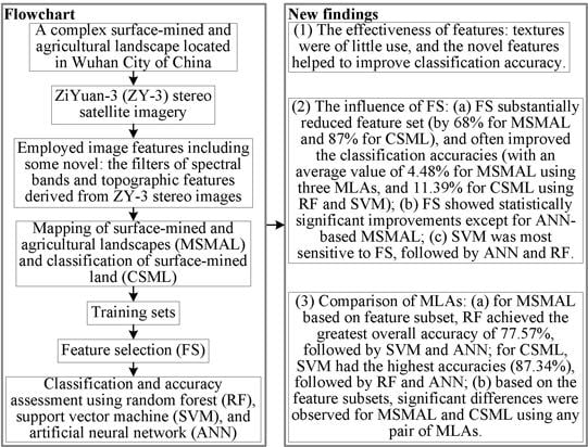
Based on the background described above, an area characterized by CSMAL, located in central China’s Wuhan City, was selected as the study area. A procedure combining a set of features derived from ZY-3 stereo imagery, a wrapper FS method, and three MLAs (RF, SVM, and ANN) was proposed and examined. This study focused on the following tasks: mapping of the surface-mined and agricultural landscapes (MSMAL), i.e., the entire study area, and classification of the surface-mined land (CSML). Four bands of ZY-3 fused imagery, the normalized difference vegetation index (NDVI) layer, principal component (PC) bands, filter features, texture measures, and topographic variables were generated. The wrapper FS method was applied to select feature subsets for subsequent classifications. The classification accuracies of MLAs were assessed and compared using all features and feature subsets, respectively. Moreover, the McNemar test was performed to examine the influences of FS and MLAs. The detailed objectives of this study were:
  • Assessing the effectiveness of the employed features. The focus was on the following: determining whether the employed features, especially the newly introduced mean and standard deviation (StDev) filters of ZY-3 spectral bands and topographic features derived from ZY-3 stereo images, are effective for classification, and which features have higher importance; whether the NDVI layer and PC bands have higher importance than spectral bands, and whether it is possible to use them separately or jointly to substitute four spectral bands for the classification tasks in this study; and for Gaussian low-pass and mean filters derived from four spectral bands with different kernel sizes, which ones result in higher importance.
  • Investigating the influence of the FS method as to how it influences the feature set and classification accuracy; whether it results in statistically significant accuracy improvements; for three MLAs, whether there are different sensitivities to FS and which one is more sensitive; and whether the land covers show different sensitivities to FS.
  • Comparing different MLAs. The aim was to examine which algorithms achieve higher performance and whether there are statistically significant differences among the three MLAs.

2. Study Area and Remote Sensing Data

The study area is located in Jiangxia District, Wuhan City, in the Hubei Province of China, and covers an area of 109.4 km2 (Figure 1). The area is characterized by typical surface-mined and agricultural landscapes. The Wulongquan mine, located in the middle of the study area, is the largest one, and is the only production base of fluxing ore for the Wuhan Iron and Steel Corporation (the world’s fourth largest steel producer). The mine extends approximately 5 km east–west and 0.3–1.5 km north–south. Exploitation began in 1958, and remains active today. In addition, agricultural and economic activity around the mine within the area includes traditional farming (rice, cotton, corn, rapeseed, and wheat), greenhouse vegetables and fruits, landscape ecological forestry, aquaculture, and village leisure tourism. The weather here is mild and moist with an annual average temperature of 15.9 °C–17.9 °C. The annual rainfall averages about 1347.7 mm with concentrated and continuous rainstorms in the rainy season. Several national road networks, including the Jing-Guang railway (connecting Beijing and Guangzhou), the Wu-Guang high-speed railway (connecting Wuhan and Guangzhou), the Wu-Xian inter-city railway (connecting Wuhan and Xianning in Hubei Province, China), the G107 (national highway 107 of China), and the Jing-Zhu expressway (connecting Beijing and Zhuhai), run north–south through the study area. There were a total of 28 field survey sample sites in the area, shown in Figure 1.
The ZY-3 image used in this study was obtained on 20 June 2012. ZY-3 is China’s first civilian high-resolution stereo mapping optical satellite, which was launched in January 2012 [30]. It has tilt and stereo mapping capability at 1:50,000 scale [31,32]. The characteristics are given in Table 1.

3. Methods

First, ZY-3 satellite data were processed, and then a set of features was employed. In accordance with the field survey, two-level land cover schemes were developed. Training sets for MSMAL and CSML were obtained based on referenced training data polygons using stratified random sampling. Subsequently, the FS method was implemented to pick out the feature subsets for MSMAL and CSML. Finally, all feature- and feature subsets-based classification models using RF, SVM, and ANN algorithms were developed, and classification accuracies were assessed. A flowchart of the process is presented in Figure 2, and details are given in the following sections.

3.1. ZY-3 Data Processing

The 3.6 m resolution front and backward looking panchromatic (PAN) data were used to extract relative digital terrain models (DTM) data with 10 m resolution using ENVI 5.0 software. The DTM was generated and used considering the following two factors: first, the height values of the ground control points in the surface-mined land changed by mining were difficult to obtain; second, it is possible for it to be only used to develop the topographic features for distinguishing land covers with heterogeneous terrain in the study area.
The 2.1 m resolution nadir-looking PAN and 5.8 m resolution nadir-looking MS images were orthorectified using a rational polynomial coefficient model and the 10 m resolution DTM. The MS image was then registered to the PAN image using a 2nd order polynomial transformation and 32 ground control points that were collected uniformly in the study area, with a root mean square error of 0.3 pixels (less than 0.5 pixels). According to our previous research, the Gram–Schmidt spectral sharpening (GS) method can achieve the best fusion performance for the mapping of surface-mined landscapes [33]. As a result, the PAN–MS image fusion for the ZY-3 satellite was achieved using the GS method. The quality of employed ZY-3 imagery was good with free clouds, and the reflectance was not adopted in the present study; the atmosphere correction thus was not conducted.

3.2. Employed Features Derived from ZY-3 Image

A total of six types of image features with different significance were employed in this study. To sum up, 106 features were available, and are listed in Table 2.
  • Basic spectral information: four spectral bands of the fused image.
  • Vegetation index: NDVI [34] that is widely used in the LCM studies was achieved.
  • PC bands: the principal component analysis is a dimensionality reduction method that can eliminate redundant information [35]. In this study, it was conducted with the four fused spectral bands. The first and second PC bands were employed with a cumulative contribution rate of 98.99%.
  • Filter features: applying the Gaussian low-pass filters to the optical image appeared to improve the mapping of surface mining and reclamation that is closely related to this study [12]. Moreover, the mean filter features of topographic data improved forested landslide detection [36,37]. As a result, this study employed and compared the Gaussian low-pass and mean filter features of the ZY-3 fused image. Furthermore, the StDev filter method that was applied to the topographic data and was shown to improve the identification of forested landslides [36,37] was used in this study. In order to assess the filter features at different scales, three kernel sizes, 3 × 3, 5 × 5, and 7 × 7 pixels, were used.
  • Texture measures: the use of texture measures has also been suggested to improve the mapping of surface mining and mine reclamation [12]. Consequently, the gray level co-occurrence matrix texture measures [38] based on the average of four texture directions were calculated in this study, including contrast, correlation, angular second moment, entropy, and homogeneity. They were also assessed at the same kernel sizes mentioned above, with offsets of 1, 2, and 3 pixels. All of the texture features were calculated for each band of the fused image.
  • Topographic variables: the use of LiDAR-derived variables improved mapping of mining and mine reclamation [13,14,15]. This study aimed to investigate whether moderate resolution topographic data derived from the stereo satellite sensors could be positive for MSMAL and CSML. Consequently, slope and aspect features were calculated from the DTM data, and the three topographic features were resampled to 2.1 m as others features.

3.3. Developing LCM Schemes

Taking into consideration existing LCM systems (national standard of China: GB/T21010-2007) and field surveys, an LCM scheme consisting of seven first-level classes was developed, namely, cropland, forestland, water, road, urban and rural residential land, bare land, and surface-mined land. Owing to CSMAL, the intra-class spectral differences increased, which might reduce the classification accuracy. For example, cropland in the study area consists of traditional cropland such as dry land with corn, vegetable and fruit greenhouse, and fallow land, which have large spectral differences. The greenhouse in the study area is a special element of the agricultural landscape, and it may be confused with other land covers with high surface albedo. As a result, in order to obtain the first-level LCM results, more detailed land cover classes representing the second-level scheme were built up. Detailed descriptions relating to the two schemes in this study are shown in Table 3.
This study focused on just two tasks: MSMAL, i.e., the first-level LCM of the entire study area, and CSML, i.e., the second-level LCM of the surface-mined land. For MSMAL, the detailed land cover classes were only used for the subsequent processes such as training set acquisition, FS, parameter optimization of classifiers, and classification model building and prediction (for details, see Section 3.4, Section 3.5 and Section 3.6). Then, the classification results were grouped into seven first-level land classes. The accuracy assessments were based on the first-level land cover scheme. For MSMAL, misclassifications among the subclasses of each first-level class were not considered. For CSML, misclassifications between surface-mined land covers and other land covers were not involved. The fine classification of second-level land cover scheme will be investigated in the future.

3.4. Obtaining Training Data

All the referenced land cover data selected as training data polygons were obtained by visual interpretation of ZY-3 satellite imagery and extensive field investigation. The surface-mined land was completely delineated. Other land cover classes were collected randomly and uniformly in the study area. For MSMAL, a stratified random sampling of equal amounts was performed on the training polygons and resulted in a training set with 2000 training samples (number of pixels) for each second-level land cover class (Table 4). For CSML, a stratified random sampling of equal fractions was performed on the referenced surface-mined land and resulted in a training set with 10% training samples (59,037, 20,614, and 18,490 pixels for opencast stope, mineral processing land, and dumping site, respectively) for each surface-mined land cover class.

3.5. FS Procedure

In this study, FS was performed using the varSelRF (variable selection using RF) package [39] in the R programming language and operating environment [40], which is a wrapper FS method. Specifically, the varSelRF package iteratively eliminates the least important variables using the out-of-bag error as the minimization criterion [41]. The number of trees for the first forest used for obtaining the initial variable rank was set as 2000. Then, in each iterative process, an RF with 500 trees was constructed without the least important 20% of the features. Afterwards, the feature subset creating the lowest out-of-bag error was selected.
FS often achieved varied feature subsets owing to different training sets. As a result, 20 randomly selected training sets for MSMAL and CSML were used for FS and resulted in 20 feature subsets, respectively. Then, for each selected feature, its selected time, mean rank, and standard deviation of the rank were drawn and ranked, in order to pick out the final feature subsets for MSMAL and CSML.

3.6. Classification Model Development and Parameter Optimization

Three MLAs were employed in this study, such as RF, SVM, and ANN. Model development and parameter optimization were implemented within the R programming language and operating environment [40].
The RF that incorporates a number of randomly generated trees [42] is an increasingly popular non-parametric ensemble learning algorithm within the remote sensing community owing to its high classification accuracy [43]. For details, see the formulas in [42] and Figure 1 in [43]. SVM is based on kernel functions and structural risk minimization theory [44]. It has been successfully used in numerous remote sensing studies [45]. To understand the theoretical background of SVM, see Figure 1 in [45]. ANN is a family of models inspired by biological nervous systems to recognize patterns and objects [46]. It also has long been used in the domain of remote sensing [47]. For specific formulas and principles, see [46]. The RF-, SVM-, and ANN-based models used the randomForest package [48], e1071 package [49], and nnet package [50], respectively.
There are actually two crucial parameters in the RF-based models, ntree (number of trees) and mtry (number of features). The former would determine the number of trees to grow and its default value of 500 was hereby used [51]. Belgiu and Drăguţ [43] reviewed the applications of the RF algorithm in remote sensing, and they suggested using the default value of 500 for ntree considering the following two factors: first, the classification accuracy was insensitive to ntree compared to mtry; second, the classification errors often stabilized before 500 trees were grown (in particular, some studies revealed that ntree did not affect the classification accuracy). The latter that would control the number of features selected for each split needs to be optimized [51]. The SVM-based models used the radial basis function (RBF) kernel and have two tuning parameters, cost and gamma. The cost parameter trades off misclassification of training examples against simplicity of the decision surface and gamma sets the width of the kernel function [52]. The multi-layer perceptron ANN with a single hidden layer was used in this study, and there are three important parameters, size, decay, and maxit [52]. The size parameter sets the number of units in the hidden layer and needs to be tuned. The decay parameter controls the weight decay, and maxit sets the maximum number of iterations; they are both left at their default values. A logistic activate/transfer function and the quasi-Newton optimization algorithm that does not use the parameters, such as learning rate and momentum, were used [50].
Classification model building and tuning were all based on the e1071 package [49], in which there is a function “best.tune” that can train and tune each of the employed MLAs. The MLAs-based models were built by the function “best.tune”, calling corresponding functions in the above-mentioned packages. A 10-fold cross-validation scheme in the function “best.tune” was used to obtain the “optimal” parameter combinations used for each classification model. First, the training set was randomly divided into 10 independent subsets of roughly equal size. Second, for each parameter combination, nine subsets were used to train the classifier and the remaining one was used for a test. This process was repeated 10 times, and the average values of the 10 overall accuracies were calculated. The “optimal” parameter settings of each algorithm were obtained based on the models that achieved the highest average overall accuracies during the cross-validation process.

3.7. Classification Accuracy Assessment

Classification accuracy was assessed based on the test data sets that were independent of the training sets. For MSMAL, based on the classification result grouped into seven first-level classes and derived from the RF algorithm and the feature subset, a stratified random sampling resulted in a test set with 700 pixels, 100 in each of the assigned classes. The referenced land cover classes of each selected pixel were determined based on visual identification of the ZY-3 imagery. All the classification algorithms and feature sets-based models were assessed based on this test set. The feature subset-based and all feature-based models for each classification algorithm were compared to evaluate the influence of FS on the classification accuracy. For CSML, all classification algorithms and feature sets-based models used the remaining 90% pixels (531,334, 185,522, and 166,408 for opencast stope, mineral processing land, and dumping site, respectively) as the test set.
The F1-measure and overall accuracy were drawn from the confusion matrix of each classification. The F1-measure is defined as the harmonic mean of the user’s accuracy and producer’s accuracy, which was used to assess the average class accuracy. A detailed description of the F1-measure can be found in Daskalaki et al. [53]. The differences in the results for the feature subset-based models and all feature-based models are quantified for the F1-measures of each class, and the overall accuracies by the percentage deviation [54]. The McNemar test is a statistical test used to compare classifier performance [55]. The test is based on chi-square statistics, computed from the error matrices of two classifications [55]. The McNemar test was used in the present study to answer the following questions: whether there are statistically significant differences between the feature subsets- and all feature-based models; and whether there are statistically significant differences among three MLAs based on the feature subsets.

4. Results

4.1. Acquisition of Feature Subsets

4.1.1. Feature Subset for MSMAL

For MSMAL, the selected feature subset is shown in Table 5 and sorted by the selected times, mean ranks, and standard deviation values of ranks. For 20 random runs, the features with selected times greater than 16 were selected. There were 34 features in the feature subset (about 32% of 106 features), which involved features from the spectral bands, vegetation index, PC bands, filter features, and topographic variables, but not texture measures. The result in Table 5 shows that: for spectral bands, only the red and near infrared (NIR) bands were selected, and the former had higher importance; the NDVI layer was of great importance and second only to DTM; all PC features were selected, and the first PC had higher importance than the spectral bands; for the same spectral band, the Gaussian low-pass and mean filter features with larger kernel sizes had greater importance; for the four spectral bands, filter features with the same kernel sizes and filter methods had different degrees of importance, the red band being the highest and green band the lowest; for the same spectral bands and kernel sizes, the mean filter features with better smoothing effect (with lower standard deviation values, see Table 6) had higher importance than the Gaussian low-pass filter features; some of the StDev filter features with large kernel size were selected; and for three topographic variables, DTM and slope were both selected, and DTM was of the highest importance.

4.1.2. Feature Subset for CSML

For CSML, the selected feature subset is presented in Table 7 and also sorted by the selected times, mean ranks, and standard deviation values of ranks. The features in the feature subset were selected every time in 20 random runs. There were only 14 features, about 13% of all the 106 features. Only some features from the vegetation index, filter features, and topographic variables were selected. Table 7 also suggests that: the NDVI layer was of the greatest importance; for the same spectral bands, the Gaussian low-pass and mean filter features with larger kernel sizes had higher importance; for the four spectral bands, the importance rank of their filter features with the same kernel sizes and filter methods, from highest to lowest, was red, green, blue, and NIR bands; for the same spectral bands and kernel sizes, the mean filter features with better smoothing effect had higher importance than the Gaussian low-pass filter features; DTM and slope were both selected, and DTM was second only to the NDVI layer.

4.2. Parameter Optimization of MLAs

4.2.1. Parameter Optimization for MSMAL

For MSMAL, four parameters of three MLAs were optimized. For feature subset- and all feature-based RF classifications, the mtry parameter ranged from 1 to 34 and 1 to 106, respectively. The “optimal” mtry values of 20 and 61 were selected, with the highest average overall accuracies of 85.77% and 84.44% for the above-mentioned two models (Table 8).
A total of 10 gamma parameters (2−15, 2−13, …, 23) and 8 values for cost parameter (2−5, 2−3, …, 29), as well as the grid search method, were used for both the feature subset-based and all feature-based models using the SVM algorithm. The “optimal” feature subset- and all feature-based models, with average overall accuracies of 86.39% and 74.19%, were achieved using gamma parameter values of 2−3 and 2−9, respectively, and the same cost parameter value of 27 (Table 8).
For feature subset- and all feature-based models using the ANN algorithm, several size parameter values (6–17 and 7–21, respectively) were examined. The same value of 16 was selected for both models, achieving average overall accuracies of 59.95% and 54.32% (Table 8).

4.2.2. Parameter Optimization for CSML

For CSML, four parameters of three MLAs were also optimized. For feature subset- and all feature-based RF classifications, the mtry parameter ranged from 1 to 14 and 1 to 106, respectively. The optimal mtry values of 12 and 95 were selected, with the highest average overall accuracies of 87.06% and 86.21% for the above-mentioned two models (Table 8).
A total of 10 gamma parameters (2−15, 2−13, …, 23) and 8 values for the cost parameter (2−5, 2−3, …, 29), as well as the grid search method, were used for both the feature subset-based and all feature-based models using the SVM algorithm. The “optimal” feature subset- and all feature-based models, with average overall accuracies of 86.63% and 71.25%, were achieved using gamma parameter values of 21 and 2−7, respectively, and the same cost parameter value of 25 (Table 8).
For feature subset- and all feature-based models using the ANN algorithm, several size parameter values (4–14 and 7–20, respectively) were examined. The maximum values of 14 and 20 were selected for two models, achieving average overall accuracies of 71.32% and 73.55% (Table 8).

4.3. Evaluation and Comparative Analysis of Classification Results

4.3.1. Visual Assessment and Analysis

Visual Assessment and Analysis for MSMAL

For MSMAL, the three classification maps derived from the feature subset-based models using the MLAs are shown in Figure 3. In the southwest and northwest corners of the study area (see the black rectangles in corresponding corners of Figure 3), the classification maps based on the ANN algorithm show some noticeable errors of commission, i.e., the misclassification of forestland as cropland. In the center (see the black rectangle above the Wulongquan mine in Figure 3) and the northeast corner (see the black rectangle in the upper right corner of Figure 3) of the study area, all three classification maps produce some commission and omission errors of the cropland and forestland classes. For the water class, a major difference in the three classification maps is present in the lower southeast quarter of the study area near the Wu-Guang high-speed railway (see the black rectangle in the lower right corner of Figure 3), which is primarily covered with water and little aquatic vegetation. For RF- and SVM-based classification maps, this area depicts water, whereas the map produced by the ANN algorithm depicts it as dominated by water dotted with patches of cropland. For the road class, the major differences in the classification maps are in the northwest corner and the southern half of the study area. The road in the northwest corner with several fish ponds (see the black inclined rectangle in the upper left corner of Figure 3) is best classified by the SVM algorithm, followed by RF, while the ANN algorithm depicts them as cropland or water. In the southern half of the study area (see the black rectangle beneath the Wulongquan mine in Figure 3), the road defined by RF and SVM shows relatively consistent visual depiction, whereas there are some noticeable errors in the ANN-based map. Some urban and rural residential land areas in the southern half of the study area (see the black rectangle in the Wulongquan Street) were misclassified as surface-mined land by three MLAs, especially the ANN algorithm. The bare land in the northeast corner of the study area (see the white inclined rectangle in the upper right corner of Figure 3) appears well-defined by RF, followed by the ANN and SVM algorithms. In the southwest (see the black rectangle in the lower left part of Figure 3) and northwest (near G107, see the black inclined rectangle in the upper left part of Figure 3) parts of the classification map produced by ANN, some surface-mined land areas were misclassified as urban and rural residential land areas. In a word, all three classification maps appeared to be relatively accurate visual depictions of the land cover classes. In particular, the RF and SVM algorithms achieved higher visual accuracy than the ANN algorithm.

Visual Assessment and Analysis for CSML

For CSML, the classification maps of the feature subset-based models using the three selected MLAs are shown in Figure 4, in which the ZY-3 fused true color image (R—Red, G—Green, B—Blue) was scaled to fit the surface-mined land. RF- and SVM-based classification maps show little visual differences, whereas there are some noticeable errors in the ANN-based map. In the southwest corner (see mine 1 in Figure 4) and southern quarter (see mine 7 in Figure 4) of the study area, the classification map derived from the ANN algorithm shows some misclassification of opencast stope as dumping site. For the northern surface-mined land (see mines 2–6 in Figure 4), there are some commission and omission errors between opencast stope and dumping site, and opencast stope and mineral processing land. In the southeast corner of the study area (see mines 9–12 in Figure 4), there are some misclassification of dumping site and mineral processing land as opencast stope. The central study area (see mine 8 in Figure 4) mainly shows some misclassification of dumping site as opencast stope or mineral processing land.

4.3.2. Accuracy Assessment and Analysis

Accuracy assessment was performed using the F1-measure, overall accuracy, percentage deviation, and statistical test for MSMAL and CSML based on the feature subsets and all features using the RF, SVM, and ANN algorithms. The location of the test samples for MSMAL is shown in Figure 5.

Overall Accuracy, F1-measure, and Percentage Deviation for MSMAL

For MSMAL, the F1-measure, overall accuracy, and percentage deviation are shown in Table 9. For the feature subset-based models, the descending order of overall accuracies was 77.57% (RF), 72.00% (SVM), and 64.29% (ANN). The same trend was observed for all feature-based models, with RF achieving the highest overall accuracy (74.86%), followed by SVM (68.00%), and ANN (61.86%). It is remarkable that the feature subset-based models achieved higher accuracies than all feature-based models. After FS, the overall accuracies increased 3.62% (RF), 5.88% (SVM), and 3.93% (ANN), resulting in an average increase of 4.48%. This phenomenon might be attributed to the elimination of irrelevant features and redundant information, and the mitigation of the curse of dimensionality. Considering that the test set was small compared to the training set, the overall accuracies for the entire data (training and test samples) by the feature subset-based models were investigated. The same order for three MLAs was observed, i.e., RF (99.61%), SVM (96.13%), and ANN (58.80%). ANN worked very bad with the training set, but achieved higher performance for the test set. The results revealed that the performance of the ANN-based model was sensitive to the test set. Moreover, the size of the test set will be further discussed in the future.
With respect to the F1-measure of each class, the RF algorithm achieved the best performance, followed by SVM and ANN for both the feature subset- and all feature-based models, with the exception of all feature-based SVM and ANN models for water; the feature subset-based models almost achieved better performance than all feature-based models for all MLAs, with five exceptions (i.e., the percentage deviations were zero or negative values): the RF algorithm for urban and rural residential land, bare land, and surface-mined land, and the ANN algorithm for water and road. In general, water and surface-mined land achieved over 80% F1-measures, with the exception of surface-mined land using an all feature-based ANN model. For three all feature-based MLAs and feature subset-based RF and SVM models, water had the highest F1-measure; however, for the feature subset-based ANN model, surface-mined land had the highest F1-measure. Road, and urban and rural residential land achieved lower F1-measures. For three all feature-based MLAs and feature subset-based SVM and ANN models, road had the lowest F1-measure; however, for the feature subset-based RF model, urban and rural residential land had the lowest F1-measure. When using RF-based models, road, and urban and rural residential land achieved 60%–70% F1-measures; however, based on SVM and ANN algorithms, they only achieved 40%–60% F1-measures. Other land cover classes achieved approximately 60%–80% F1-measures, with the exception of cropland using the all feature-based ANN model. The low accuracies of parameter optimization and test set classification for ANN models might be attributed to the local convergence issue due to the small training set for MSMAL.
For different land covers, there were different sensitivities to FS. The percentage deviation values shown in Table 9 confirmed the following. With regard to the RF algorithm, the largest accuracy deviations were observed for road (13.19%), followed by cropland (8.44%), forestland (6.57%), and urban and rural residential land (−5.01%); only little or no deviations were found for surface-mined land (−1.62%), water (1.58%), and bare land (0%). With regard to the SVM algorithm, the largest accuracy increases were observed for road (18.93%), followed by forestland (9.44%), and water (5.01%); only little enhancement was achieved for cropland (3.16%), urban and rural residential land water (3.08%), surface-mined land (2.97%), and bare land (1.46%). With regard to the ANN algorithm, the outstanding accuracy deviations were observed for forestland (9.82%), road (−8.37%), and cropland (7.47%), followed by surface-mined land (5.08%); only small deviations were found for water (−3.58%), bare land (2.51%), and urban and rural residential land water (2.02%).

McNemar Test for MSMAL

For MSMAL, the McNemar test was performed for each pair of predictions made by feature subset- and all feature-based models using RF, SVM, and ANN algorithms. Table 10 shows the results containing the numbers of cases that were wrongly classified by classifier i but correctly classified by classifier j (i, j = 1, 2), chi-square values, and the p value. The McNemar test revealed that: based on the feature subset, the statistically significant differences were observed between RF and SVM algorithms (p < 0.001), RF and ANN algorithms (p < 0.001), and SVM and ANN algorithms (p < 0.01); there were significant differences (p < 0.05) between the feature subset- and all feature-based RF and SVM models; the observed difference between the feature subset- and all feature-based ANN models was not statistically significant (0.005 < p < 0.25).

Overall Accuracy, F1-Measure, and Percentage Deviation for CSML

For CSML, the F1-measure, overall accuracy, and percentage deviation are shown in Table 11. For the feature subset-based models, the descending order of overall accuracies was 87.34% (SVM), 87.18% (RF), and 71.88% (ANN). However, for all feature-based models, the RF algorithm achieved the highest overall accuracy (86.41%), followed by ANN (73.51%) and SVM (71.66%). The feature subset-based models achieved better performance than all feature-based models when using RF and SVM algorithms, and conversely for ANN. After FS, the overall accuracies increased 0.89% and 21.88% when using RF and SVM algorithms, respectively, but decreased 2.22% when using the ANN algorithm.
With respect to the F1-measure of each class, the same trends of overall accuracies were observed: for the feature subset-based models, the SVM algorithm achieved the best performance, followed by RF and ANN; for all feature-based models, the performance in descending order was RF, ANN, and SVM. In general, opencast stope achieved approximately 81%–92% F1-measures for all the models. Mineral processing land and dumping site achieved lower F1-measures. When using feature subset-based RF and SVM models and the all feature-based RF model, mineral processing land and dumping site achieved approximately 77%–82% F1-measures. However, when using feature subset-based ANN, all feature-based SVM and ANN models, they only achieved 50%–60% F1-measures. The relative low accuracies of parameter optimization and test set classification for ANN models might be attributed to overfitting due to the large training set with high dimension for CSML.
For different surface-mined land covers, there were different sensitivities to FS. The percentage deviation values shown in Table 11 confirm the following. With regard to the RF algorithm, the largest accuracy deviation was observed for dumping site (3.12%), only small deviations were achieved for opencast stope (0.51%) and mineral processing land (0.80%). With regard to the SVM algorithm, enormous accuracy increases were observed for dumping site (58.60%), followed by mineral processing land (44.64%) and opencast stope (12.51%). With regard to the ANN algorithm, the largest accuracy decrease was observed for dumping site (11.03%), followed by mineral processing land (3.44%) and opencast stope (1.00%).

McNemar Test for CSML

For CSML, the McNemar test was performed for each pair of classifications made by feature subset-based and all feature-based models using RF, SVM, and SVM algorithms. Table 12 shows the results containing the numbers of cases that were wrongly classified by classifier i but correctly classified by classifier j (i, j = 1, 2), and chi-square values. The chi-square values were much larger than 10.83 (i.e., p < 0.001), thus all the tests were statistically significant. In short, there were statistically significant differences for the feature subset- and all feature-based models using the same classification algorithms, and there were statistically significant differences among the three MLAs based on the feature subset.

5. Discussion

5.1. Effectiveness of Employed Features

5.1.1. Vegetation Index and PC Bands

The relevant studies of complex surface-mined landscapes [12,13,14,15] and complex agricultural landscapes [8,9,10,11] have not used vegetation indices and PC bands. In this study, the FS result for MSMAL showed that NDVI and the first PC had higher importance than the selected red and NIR bands. The feature subset selected for CSML included the NDVI layer, and the PC and spectral bands with lower importance were not selected. A similar result, that vegetation index, such as the red-edge adaptation of NDVI (NDVI-RE, derived from the red-edge and NIR bands of the RapidEye image), achieved higher importance than spectral bands was reported in the study of classifying the insect defoliation levels [56]. Moreover, the study showed that using only NDVI-RE outperformed using all five bands. Considering that both the NDVI layer and PC bands were derived from the linear computation of spectral bands, two additional experiments were added to further investigate whether NDVI and PC bands could be separately or jointly used to substitute the spectral bands for classification tasks in this study: comparison of four feature sets for MSMAL using the RF algorithm (four spectral bands, NDVI, first PC, and both NDVI and first PC) and comparison of four spectral bands and NDVI for CSML using the RF algorithm. The results showed that, although NDVI and first PC achieved higher importance than the four spectral bands, separately or jointly using them did not result in higher classification accuracies than using all the spectral bands. This shows that whether NDVI and PC bands could be separately or jointly used to substitute the spectral bands for classification tasks depends on the specific applications.

5.1.2. Filter Features

Among the mentioned relevant studies of complex landscapes [8,9,10,11,12,13,14,15], only Maxwell et al. [12] used the Gaussian low-pass filters, and their study suggested that filter features produced greater accuracy improvements than texture measures, and those with larger kernel size resulted in higher accuracy and statistically significant improvements. In this study, the Gaussian low-pass and mean filter features similarly outperformed texture measures. Besides, this study revealed that the effectiveness of filter features depended on the filter methods, kernel sizes, and derived variables. Filter features with the mean filter method, larger kernel sizes, and derivation from the red band had greater importance. The StDev filter features produced based on LiDAR derivatives were shown to be useful for landslide identification [36,37]. Similarly, in this study, the StDev filter features derived from ZY-3 data also appeared to be effective.

5.1.3. Texture Measures

Texture measures derived from spectral bands have been investigated to improve accuracy for LCM in some relevant studies with complex landscapes [9,10,12] and other studies [17,57]. Moreover, texture measures derived from topographic data appeared to be positive for classification tasks within the rugged terrain area [36,58]. However, Maxwell et al. [14] revealed that object texture measures produced based on optical imagery decreased the classification accuracy of mining and mine reclamation. Furthermore, Li et al. [37] reported that no object features based on the pixel layer of textures were selected after FS, which suggested that the texture features might be of little use for object-based forested landslide identification. Similarly, in this study, the feature subset did not involve texture measures, suggesting that texture measures provided little or no effective information for classification. In general, the effectiveness of texture measures depended on the specific applications and input data.

5.1.4. Topographic Variables

ASTER GDEM helped to improve the classification of a shifting cultivation landscape [9] and LiDAR-derived topographic features improved the classification accuracy for the mapping of mining and mine reclamation [13,14,15] and for forested landslide identification in the rugged terrain area [36,37,58]. In this study, easily produced DTM and its derivatives based on the front and backward looking bands of the ZY-3 were similarly indicated to be useful for MSMAL and CSML. Furthermore, the topographic textures should be positive and will be investigated in the future.

5.2. Influences of Sampling Design for Training Sets, FS Method, Size of Test Set, and Comparison of MLAs

5.2.1. Class-Specific Classification Accuracy and Influences of Sampling Design for Training Sets and the FS Method

For specific classes, different algorithms and feature sets resulted in varied classification accuracies. For MSMAL, water and surface-mined land achieved higher F1-measures; road, and urban and rural residential land achieved lower accuracies; cropland, forestland, and bare land achieved moderate accuracies. Water usually can be easily classified. With respect to surface-mined land, the topographic data and sampling design for surface-mined land, which suffered some of the effects of spatial auto-correlation [36], contributed jointly to the classification accuracy. The lower accuracies of road, and urban and rural residential land were attributed to the confusion between themselves and with other land covers. The high accuracies for CSML to some degree can be ascribed to the use of a big training set and the effect of spatial auto-correlation owing to the sampling design [36]. The opencast stope with obvious negative terrain achieved the highest accuracies, followed by mineral processing land with some linear characteristics of mineral processing facilities, and dumping site.
With respect to class-specific F1-measure deviations between feature subsets- and all feature-based models, the influence of FS strongly depended on the investigated land cover classes and classification algorithms. For MSMAL, the classes with higher (lower) F1-measures generally resulted in lower (higher) deviations. For example, road had low F1-measures and highest deviations when using RF and SVM algorithms (13.19% and 18.93%, respectively). Similarly, for CSML, opencast stope achieved the highest F1-measures and lowest deviations, and conversely, dumping site achieved the lowest F1-measures and highest deviations. Therefore, a conclusion similar to that of Schuster et al. [54] could be drawn, i.e., that the land cover classes that were more easily classified were less sensitive to FS.

5.2.2. Influence of FS on Feature Set and Overall Classification Accuracy

In this study, the FS method not only significantly reduced the feature sets by 68% for MSMAL and 87% for CSML, but also improved the accuracies of MSMAL with an average value of 4.48% for the three selected MLAs. However, FS improved the accuracies of CSML with an average value of 11.39% for RF and SVM algorithms, with only one exception of using ANN with a decrease of 2.22%. Similarly, Duro et al. [59] showed that FS could reduce the number of variables (about 37%–62%) and resulted in a slight decrease (<0.5%) and two small increases (<1.5%) for LCM by using RF-based models combined with different remote sensing data sets. However, some studies showed that FS always improved the classification. For example, Maxwell et al. [12] reported that utilizing the top 10% of variables selected using an FS method based on variable importance measures for RF resulted in significant improvement for the mapping of mining and mine reclamation. Moreover, in the study of pixel-based forested landslide detection [36], FS achieved slight improvement by using the RF algorithm (about 0.44%) and marked reduction of the feature set (about 74%); for object-based forested landslide identification [37], FS achieved varied increases for RF and SVM (0.86% and 2.34%, respectively), and remarkably reduced the dimensionality of the feature set (about 90%). In general, FS could significantly reduce the features set, and in most cases improve the classification accuracy. Parameter optimization for the FS method used might further improve its performance.

5.2.3. Comparison of MLAs and Their Sensitivities to FS

It can be concluded in this study that: for MSMAL using both feature subset and all features, the RF algorithm had the greatest classification accuracies, followed by SVM and ANN; for CSML using both feature subset and all features, RF achieved higher accuracies than ANN; however, the SVM algorithm that might be subject to the model parameters obtained either the highest (feature subset-based model) or lowest (all feature-based model) classification accuracies; for both MSMAL and CSML, the SVM algorithm was most sensitive to FS, followed by ANN and RF.
With respect to the comparison of MLAs, previous studies showed some similar results. For example, RF and SVM algorithms have been shown to obtain comparable accuracies for LCM [29,60]. RF was more capable of processing the highly correlated terrain features [13,61] and has outperformed SVM in mapping forested landslides [37]. Cracknell and Reading [52] suggested that RF and SVM outperform ANN, especially when handling data sets with small numbers of training samples and large numbers of variables and/or classes. Moreover, the relevant studies of complex surface-mined landscapes [12,14,15] suggested that SVM provided more accurate classifications of surface mining and mine reclamation than the RF algorithm. In most cases, RF and SVM showed similar classification abilities and varied in different classification tasks, and they often outperformed the ANN algorithm.
With respect to the sensitivities of MLAs to FS, the result drawn in this study was consistent with previous studies. For example, Chen et al. [36] and Duro et al. [59] suggested that RF showed relatively low sensitivity to the FS procedure. Moreover, the SVM algorithm was more sensitive to the FS procedure than RF for object-based forested landslide identification [37]. Svetnik et al. [62] revealed that RF was less sensitive to FS than ANN and SVM. The RF algorithm is capable of handling high-dimension datasets (i.e., with lower sensitivity to FS) because of the ensemble of multiple tree classifiers on random subsets of training samples and features [43,62]. However, SVM suffered from the effect of outliers on the construction of optimal decision boundary [45], and ANN may be trapped by overfitting and local convergence as a result of high dimension datasets with irrelevant features or redundant information [63]. To sum up, it could be concluded that the sensitivities of MLAs to FS depend on the algorithm itself, rather than the classification ability and specific applications.

5.2.4. Assessing Whether There Are Statistically Significant Differences after FS and among MLAs

Statistical tests have been employed to compare the performance of different FS methods [12,28], classifiers [14,15,29,64], image analysis methods [29], and varied remote sensing data sets [12,13,14].
Maxwell et al. [12] assessed a filter FS method and revealed that combining the filter method and the RF algorithm caused a statistically significant accuracy increase for the mapping of mining and mine reclamation. In addition, Fassnacht et al. [28] suggested that the wrapper FS methods often achieved higher performance than filter methods. As a result, this study first investigated whether a wrapper FS method could significantly improve the accuracies of MSMAL and CSML based on RF, SVM, and ANN algorithms. The result suggested a conclusion similar to that of Maxwell et al. [12], that the wrapper method could significantly improve the accuracies of MSMAL for both RF and SVM algorithms, and the accuracies of CSML for all three MLAs. However, it is noted that there was no significant difference between feature subset- and all feature-based ANN models. The cause might be that the feature subset remained too large for ANN, or ANN was trapped in local convergence because of the small training set for MSMAL. In general, for MSMAL and CSML, FS usually resulted in significant accuracy improvements by using advanced MLAs such as RF and SVM.
Based on the feature subsets, statistically significant differences were observed for both MSMAL and CSML using any pair of MLAs. For MSMAL, the RF algorithm significantly outperformed the other two algorithms, and the SVM algorithm significantly outperformed the ANN algorithm. For CSML, the SVM algorithm significantly outperformed the other two algorithms, and the RF algorithm significantly outperformed the ANN algorithm. Some studies on the mapping of mining and mine reclamation that were closely related to this study showed similar conclusions. For example, Maxwell et al. [14] showed that SVM significantly outweighed RF, Boosted CART, and KNN. Maxwell et al. [15] also showed that SVM produced significantly higher classification accuracy than the ensemble tree algorithms. To sum up, RF and SVM often significantly outperformed other algorithms; and which was better and whether there were statistically significant differences between the two algorithms depended on the specific studies.

5.2.5. Size of Test Set for Statistical Test

The determination of test set size is often subjective. As suggested by Foody [65], the size of a test set was very important with respect to accuracy assessment and comparison. Moreover, Duro et al. [29] reported that a too small test set would not be able to evaluate the statistical differences of the classification accuracies derived from different MLAs and image analysis methods. However, the exact size of test set that is suitable for the assessment of statistical differences is difficult to determine, and there is no well-established and effective method, especially since the appropriate size of the test set may vary with the classification task and study area. As a result, for specific classification, it may not make sense to study which size of test set is optimal, and effort should be instead focused on determining whether the test set is sufficient. In this study, a small test set and a massive test set were used and examined for MSMAL and CSML, respectively. The results of the statistical test showed that although the test set for MSMAL was small, it was enough to assess the statistically meaningful differences of the classifications present in this study, and the massive test set for CSML offered an exact result with unnecessary precision.

6. Conclusions

The present study focused on LCM in an area characterized by CSMAL located in Wuhan City, central China, based on ZY-3 stereo satellite imagery. First, a set of features were employed involving four bands of a ZY-3 fused image, the NDVI layer, PC bands, filter features, texture measures, and topographic variables. The mean and StDev filter features derived from ZY-3 spectral bands and topographic data derived from stereo images were first applied. Based on these features, the FS method and three MLAs were examined for MSMAL and CSML, respectively. Moreover, the McNemar test was performed to examine the influences of FS and MLAs. The following conclusions were drawn.
  • The effectiveness of the employed features. For MSMAL, all types of features except textures were useful. For CSML, only some features from vegetation index, filter features, and topographic variables were useful. For MSMAL, although NDVI and first PC achieved higher importance than the four spectral bands, separately or jointly using them could not result in higher classification accuracies than using all the spectral bands. Similarly, for CSML, although NDVI achieved higher importance than the spectral bands, using it did not result in higher classification accuracies compared to using all the spectral bands. For both MSMAL and CSML, filter features with the mean filter method, larger kernel sizes, and derivation from the red band had greater importance.
  • The influence of the FS method. The FS method not only substantially reduced the feature sets by 68% for MSMAL and 87% for CSML, but also improved the accuracies of MSMAL, with an average value of 4.48% for the selected three MLAs. However, FS improved the accuracies of CSML, with an average value of 11.39% for the RF and SVM algorithms, with only one exception when using ANN, with a decrease of 2.22%. FS could significantly improve the classification accuracies of MSMAL for both the RF and SVM algorithms, and the accuracies of CSML for all three MLAs. However, it is noted that there was no significant difference between the feature subset- and all feature-based ANN model for MSMAL. For both MSMAL and CSML, the SVM algorithm was most sensitive to FS, followed by ANN and RF. Comparison of MLAs. For MSMAL using feature subset and all features, the RF algorithm had the greatest classification accuracies (with an overall accuracy of 77.57% based on feature subset), followed by SVM (72.00%) and ANN (64.29%). For CSML, RF (87.18%) achieved higher accuracies than ANN (71.88%); however, the SVM algorithm (87.34%) obtained either the highest (feature subset-based model) or lowest (all feature-based model) classification accuracies. Based on the feature subsets, statistically significant differences were observed for both MSMAL and CSML by using any pair of MLAs; for MSMAL, the RF algorithm significantly outperformed the other two algorithms, and the SVM algorithm significantly outperformed the ANN algorithm; for CSML, the SVM algorithm significantly outperformed the other two algorithms, and the RF algorithm significantly outperformed the ANN algorithm.
In general, the proposed approach combining a set of effective spectral and topographic features derived from ZY-3 stereo imagery, a wrapper FS method helping to substantially reduce the feature set and in most cases improve the classification accuracy, and three high performance MLAs contributed to both MSMAL and CSML in the CSMAL. In the future, the following aspects will be focused on: other effective texture measures based on stereo satellite imagery; the class imbalance issue; the effect of different test set sizes on classification accuracy; object-based fine mapping of the second-level land cover scheme; comparison and integration of feature reduction methods; and the ensemble learning algorithms for mapping of similar complex landscapes.

Acknowledgments

This research was jointly supported by the Fundamental Research Funds for Central Universities, China University of Geosciences (Wuhan) (No. CUGL150417), the China Geological Survey (No. 12120115063201), and the China Scholarship Council (No. 201406415051).

Author Contributions

All authors have made significant contributions to the manuscript. Xianju Li and Weitao Chen conceived of, designed, and performed the experiments and wrote the manuscript. Xinwen Cheng and Lizhe Wang helped to analyze the results and revise the manuscript.

Conflicts of Interest

The authors declare no conflict of interest.

References

  1. Gong, P.; Wang, J.; Yu, L.; Zhao, Y.C.; Zhao, Y.Y.; Liang, L.; Niu, Z.; Huang, X.; Fu, H.; Liu, S.; et al. Finer resolution observation and monitoring of global land cover: First mapping results with Landsat TM and ETM+ data. Int. J. Remote Sens. 2013, 34, 2607–2654. [Google Scholar] [CrossRef]
  2. Sellers, P.J.; Meeson, B.W.; Hall, F.G.; Asrar, G.; Murphy, R.E.; Schiffer, R.A.; Bretheron, F.P.; Dickinson, R.E.; Ellingson, R.G.; Huemmrich, K.F.; et al. Remote sensing of the land surface for studies of global change: Models—Algorithms—Experiments. Remote Sens. Environ. 1995, 51, 3–26. [Google Scholar] [CrossRef]
  3. Myint, S.W.; Gober, P.; Brazel, A.; Grossman-Clarke, S.; Weng, Q. Per-pixel vs. object-based classification of urban land cover extraction using high spatial resolution imagery. Remote Sens. Environ. 2011, 115, 1145–1161. [Google Scholar] [CrossRef]
  4. Senf, C.; Leitão, P.J.; Pflugmacher, D.; van der Linden, S.; Patrick, H. Mapping land cover in complex Mediterranean landscapes using Landsat: Improved classification accuracies from integrating multi-seasonal and synthetic imagery. Remote Sens. Environ. 2015, 156, 527–536. [Google Scholar] [CrossRef]
  5. Yan, W.Y.; Shaker, A.; El-Ashmawy, N. Urban land cover classification using airborne LiDAR data: A review. Remote Sens. Environ. 2015, 158, 295–310. [Google Scholar] [CrossRef]
  6. Li, M.; Bijker, W.; Stein, A. Use of binary partition tree and energy minimization for object-based classification of urban land cover. ISPRS J. Photogramm. Remote Sens. 2015, 102, 48–61. [Google Scholar] [CrossRef]
  7. Niemeyer, J.; Rottensteiner, F.; Soergel, U. Contextual classification of lidar data and building object detection in urban areas. ISPRS J. Photogramm. Remote Sens. 2014, 87, 152–165. [Google Scholar] [CrossRef]
  8. Goodin, D.G.; Anibas, K.L.; Bezymennyi, M. Mapping land cover and land use from object-based classification: An example from a complex agricultural landscape. Int. J. Remote Sens. 2015, 36, 4702–4723. [Google Scholar] [CrossRef]
  9. Hurni, K.; Hett, C.; Epprecht, M.; Messerli, P.; Heinimann, A. A texture-based land cover classification for the delineation of a shifting cultivation landscape in the Lao PDR using landscape metrics. Remote Sens. 2013, 5, 3377–3396. [Google Scholar] [CrossRef]
  10. Okubo, S.; Parikesit; Muhamad, D.; Harashina, K.; Takeuchi, K.; Umezaki, M. Land use/cover classification of a complex agricultural landscape using single-dated very high spatial resolution satellite-sensed imagery. Can. J. Remote Sens. 2010, 36, 722–736. [Google Scholar] [CrossRef]
  11. Piiroinen, R.; Heiskanen, J.; Mõttus, M.; Pellikka, P. Classification of crops across heterogeneous agricultural landscape in Kenya using AisaEAGLE imaging spectroscopy data. Int. J. Appl. Earth Obs. Geoinf. 2015, 39, 1–8. [Google Scholar] [CrossRef]
  12. Maxwell, A.E.; Strager, M.P.; Warner, T.A.; Zegre, N.P.; Yuill, C.B. Comparison of NAIP orthophotography and RapidEye satellite imagery for mapping of mining and mine reclamation. GIScience Remote Sens. 2014, 51, 301–320. [Google Scholar] [CrossRef]
  13. Maxwell, A.E.; Warner, T.A. Differentiating mine-reclaimed grasslands from spectrally similar land cover using terrain variables and object-based machine learning classification. Int. J. Remote Sens. 2015, 36, 4384–4410. [Google Scholar] [CrossRef]
  14. Maxwell, A.E.; Warner, T.A.; Strager, M.P.; Conley, J.F.; Sharp, A.L. Assessing machine-learning algorithms and image- and Lidar-derived variables for GEOBIA classification of mining and mine reclamation. Int. J. Remote Sens. 2015, 36, 954–978. [Google Scholar] [CrossRef]
  15. Maxwell, A.E.; Warner, T.A.; Strager, M.P.; Pal, M. Combining RapidEye satellite imagery and Lidar for mapping of mining and mine reclamation. Photogramm. Eng. Remote Sens. 2014, 80, 179–189. [Google Scholar] [CrossRef]
  16. Alrababah, M.A.; Alhamad, M.N. Land use/cover classification of arid and semi-arid Mediterranean landscapes using Landsat ETM. Int. J. Remote Sens. 2006, 27, 2703–2718. [Google Scholar] [CrossRef]
  17. Rodriguez-Galiano, V.F.; Chica-Olmo, M.; Abarca-Hernandez, F.; Atkinson, P.M.; Jeganathan, C. Random forest classification of Mediterranean land cover using multi-seasonal imagery and multi-seasonal texture. Remote Sens. Environ. 2012, 121, 93–107. [Google Scholar] [CrossRef]
  18. Yüksel, A.; Akay, A.E.; Gundogan, R. Using ASTER imagery in land use/cover classification of eastern Mediterranean landscapes according to CORINE land cover project. Sensors 2008, 8, 1237–1251. [Google Scholar] [CrossRef]
  19. Adam, E.; Mutanga, O.; Odindi, J.; Abdel-Rahman, E.M. Land-use/cover classification in a heterogeneous coastal landscape using RapidEye imagery: Evaluating the performance of random forest and support vector machines classifiers. Int. J. Remote Sens. 2014, 35, 3440–3458. [Google Scholar] [CrossRef]
  20. Paneque-Gálvez, J.; Mas, J.F.; Moré, G.; Cristóbal, J.; Orta-Martínez, M.; Luz, A.C.; Guèzea, M.; Macíae, M.J.; Reyes-Garcíaf, V. Enhanced land use/cover classification of heterogeneous tropical landscapes using support vector machines and textural homogeneity. Int. J. Appl. Earth Obs. Geoinf. 2013, 23, 372–383. [Google Scholar] [CrossRef]
  21. Palmer, M.A.; Bernhardt, E.S.; Schlesinger, W.H.; Eshleman, K.N.; Foufoula-Georgiou, E.; Hendryx, M.S.; Lemly, A.D.; Likens, G.E.; Loucks, O.L.; Power, M.E.; et al. Mountaintop mining consequences. Science 2010, 327, 148–149. [Google Scholar] [CrossRef] [PubMed]
  22. Townsend, P.A.; Helmers, D.P.; Kingdon, C.C.; McNeil, B.E.; de Beurs, K.M.; Eshleman, K.N. Changes in the extent of surface mining and reclamation in the Central Appalachians detected using a 1976–2006 Landsat time series. Remote Sens. Environ. 2009, 113, 62–72. [Google Scholar] [CrossRef]
  23. Wickham, J.D.; Riitters, K.H.; Wade, T.G.; Coan, M.; Homer, C. The effect of Appalachian mountaintop mining on interior forest. Landsc. Ecol. 2007, 22, 179–187. [Google Scholar] [CrossRef]
  24. Butler, S.J.; Vickery, J.A.; Norris, K. Farmland biodiversity and the footprint of agriculture. Science 2007, 315, 381–384. [Google Scholar] [CrossRef] [PubMed]
  25. Forman, R.T.T.; Godron, M. Landscape Ecology; Wiley, Inc.: New York, NY, USA, 1986. [Google Scholar]
  26. Smiraglia, D.; Ceccarelli, T.; Bajocco, S.; Perini, L.; Salvati, L. Unraveling landscape complexity: Land use/land cover changes and landscape pattern dynamics (1954–2008) in contrasting peri-urban and agro-forest regions of northern Italy. Environ. Manag. 2015, 56, 916–932. [Google Scholar] [CrossRef] [PubMed]
  27. Chan, J.C.W.; Paelinckx, D. Evaluation of Random Forest and Adaboost tree-based ensemble classification and spectral band selection for ecotope mapping using airborne hyperspectral imagery. Remote Sens. Environ. 2008, 112, 2999–3011. [Google Scholar] [CrossRef]
  28. Fassnacht, F.E.; Neumann, C.; Förster, M.; Buddenbaum, H.; Ghosh, A.; Clasen, A.; Joshi, P.K.; Koch, B. Comparison of feature reduction algorithms for classifying tree species with hyperspectral data on three central European test sites. IEEE J. Sel. Top. Appl. Earth Obs. Remote Sens. 2014, 7, 2547–2561. [Google Scholar] [CrossRef]
  29. Duro, D.C.; Franklin, S.E.; Dubé, M.G. A comparison of pixel-based and object-based image analysis with selected machine learning algorithms for the classification of agricultural landscapes using SPOT-5 HRG imagery. Remote Sens. Environ. 2012, 118, 259–272. [Google Scholar] [CrossRef]
  30. Huang, X.; Wen, D.; Xie, J.; Zhang, L. Quality assessment of panchromatic and multispectral image fusion for the ZY-3 satellite: From an information extraction perspective. IEEE Geosci. Remote Sens. Lett. 2014, 11, 753–757. [Google Scholar] [CrossRef]
  31. Dong, Y.; Chen, W.; Chang, H.-C.; Zhang, Y.; Feng, R.; Meng, L. Assessment of orthoimage and DEM derived from ZY-3 stereo image in Northeastern China. Surv. Rev. 2015. [Google Scholar] [CrossRef]
  32. Gao, M.-L.; Zhao, W.-J.; Gong, Z.-N.; Gong, H.-L.; Chen, Z.; Tang, X.-M. Topographic correction of ZY-3 satellite images and its effects on estimation of shrub leaf biomass in mountainous areas. Remote Sens. 2014, 6, 2745–2764. [Google Scholar] [CrossRef]
  33. Chen, W.; Zhang, L.; Zhang, Z.; Wang, Y. Comparison of fusion imageries with spectral fidelity using SPOT5. Proc. SPIE 2009. [Google Scholar] [CrossRef]
  34. Goward, S.N.; Markham, B.; Dye, D.G.; Dulaney, W.; Yang, J. Normalized difference vegetation index measurements from the Advanced Very High Resolution Radiometer. Remote Sens. Environ. 1991, 35, 257–277. [Google Scholar] [CrossRef]
  35. Pearson, K. On lines and planes of closest fit to systems of points in space. Philos. Mag. 1901, 2, 559–572. [Google Scholar] [CrossRef]
  36. Chen, W.; Li, X.; Wang, Y.; Chen, G.; Liu, S. Forested landslide detection using LiDar data and the random forest algorithm: A case study of the Three Gorges, China. Remote Sens. Environ. 2014, 152, 291–301. [Google Scholar] [CrossRef]
  37. Li, X.; Cheng, X.; Chen, W.; Chen, G.; Liu, S. Identification of forested landslides using LiDar data, object-based image analysis, and machine learning algorithms. Remote Sens. 2015, 7, 9705–9726. [Google Scholar] [CrossRef]
  38. Haralick, R.M.; Shanmugam, K.; Dinstein, I.H. Textural features for image classification. IEEE Trans. Syst. Man Cybern. 1973, SMC-3, 610–621. [Google Scholar] [CrossRef]
  39. Diaz-Uriarte, R. Varselrf: Variable Selection Using Random Forests; R Package Version 0.7-3; TU Wien: Vienna, Austria, 2010. [Google Scholar]
  40. R Development Core Team. R: A Language and Environment for Statistical Computing; R Foundation for Statistical Computing: Vienna, Austria, 2013. [Google Scholar]
  41. Diaz-Uriarte, R.; de Andres, S.A. Gene selection and classification of microarray data using random forest. BMC Bioinform. 2006, 7, 3. [Google Scholar] [CrossRef] [PubMed]
  42. Breiman, L. Random forests. Mach. Learn. 2001, 45, 5–32. [Google Scholar] [CrossRef]
  43. Belgiu, M.; Drăguţ, M. Random forest in remote sensing: A review of applications and future directions. ISPRS J. Photogramm. Remote Sens. 2016, 114, 24–31. [Google Scholar] [CrossRef]
  44. Vapnik, V. The Nature of Statistical Learning Theory; Springer-Verlag, Inc.: New York, NY, USA, 1995. [Google Scholar]
  45. Mountrakis, G.; Im, J.; Ogole, C. Support vector machines in remote sensing: A review. ISPRS J. Photogramm. Remote Sens. 2011, 66, 247–259. [Google Scholar] [CrossRef]
  46. Rojas, R. Neural Netwoks: A Systematic Introduction; Springer-Verlag, Inc.: New York, NY, USA, 1996. [Google Scholar]
  47. Shao, Y.; Lunetta, R. Comparison of support vector machine, neural network, and CART algorithms for the land-cover classification using limited training data points. ISPRS J. Photogramm. Remote Sens. 2012, 70, 78–87. [Google Scholar] [CrossRef]
  48. Liaw, A.; Wiener, M. Classification and regression by RandomForest. R News 2002, 2, 18–22. [Google Scholar]
  49. Meyer, D.; Dimitriadou, E.; Hornik, K.; Weingessel, A.; Leisch, F. E1071: Misc Functions of the Department of Statistics (e1071); R Package Version 1.6-4; TU Wien: Vienna, Austria, 2014. [Google Scholar]
  50. Venables, W.N.; Ripley, B.D. Model Applied Statistics with S; Springer-Verlag, Inc.: New York, NY, USA, 2002. [Google Scholar]
  51. Breiman, L.; Cutler, A. Random Forests Leo Breiman and Adele Cutler—Classification/Clustering—Description. Available online: http://www.stat.berkeley.edu/~breiman/RandomForests/cc_home.htm (accessed on 22 March 2016).
  52. Cracknell, M.J.; Reading, A.M. Geological mapping using remote sensing data: A comparison of five machine learning algorithms, their response to variations in the spatial distribution of training data and the use of explicit spatial information. Comput. Geosci. 2014, 63, 22–33. [Google Scholar] [CrossRef]
  53. Daskalaki, S.; Kopanas, I.; Avouris, N. Evaluation of classifiers for an uneven class distribution problem. Appl. Artif. Intell. 2006, 20, 381–417. [Google Scholar] [CrossRef]
  54. Schuster, C.; Förster, M.; Kleinschmit, B. Testing the red edge channel for improving land-use classifications based on high-resolution multi-spectral satellite data. Int. J. Remote Sens. 2012, 33, 5583–5599. [Google Scholar] [CrossRef]
  55. Manandhar, R.; Odeh, I.O.A.; Ancev, T. Improving the accuracy of land use and land cover classification of Landsat data using post-classification enhancement. Remote Sens. 2009, 1, 330–344. [Google Scholar] [CrossRef]
  56. Adelabu, S.; Mutanga, O.; Adam, E. Evaluating the impact of red-edge band from Rapideye image for classifying insect defoliation levels. ISPRS J. Photogramm. Remote Sens. 2014, 95, 34–41. [Google Scholar] [CrossRef]
  57. Ghimire, B.; Rogan, J.; Miller, J. Contextual land-cover classification: incorporating spatial dependence in land-cover classification models using random forests and the Getis statistic. Remote Sens. Lett. 2010, 1, 45–54. [Google Scholar] [CrossRef]
  58. Chen, G.; Li, X.; Chen, W.; Cheng, X.; Zhang, Y.; Liu, S. Extraction and application analysis of landslide influential factors based on LiDar DEM: A case study in the Three Gorges area, China. Nat. Hazards 2014, 74, 509–526. [Google Scholar] [CrossRef]
  59. Duro, D.C.; Franklin, S.E.; Dube, M.G. Multi-scale object-based image analysis and feature selection of multi-sensor Earth Observation imagery using random forests. Int. J. Remote Sens. 2012, 33, 4502–4526. [Google Scholar] [CrossRef]
  60. Pal, M. Random forest classifier for remote sensing classification. Int. J. Remote Sens. 2005, 26, 217–222. [Google Scholar] [CrossRef]
  61. Burkholder, A.; Warner, T.A.; Culp, M.; Landenberger, R.E. Seasonal trends in separability of leaf reflectance spectra for Ailanthus altissima and four other tree species. Photogramm. Eng. Remote Sens. 2011, 77, 793–804. [Google Scholar] [CrossRef]
  62. Svetnik, V.; Liaw, A.; Tong, C.; Wang, T. Application of Breiman’s random forest to modeling structure-activity relationships of pharmaceutical molecules. In Multiple Classifier Systems; Roli, F., Kittler, J., Windeatt, T., Eds.; Springer: Berlin, Germany; Heidelberg, Germany, 2004; pp. 334–343. [Google Scholar]
  63. Foody, G.M.; Arora, M.K. An evaluation of some factors affecting the accuracy of classification by an artificial neural network. Int. J. Remote Sens. 1997, 18, 799–810. [Google Scholar] [CrossRef]
  64. Rozenstein, O.; Karnieli, A. Comparison of methods for land-use classification incorporating remote sensing and GIS inputs. Appl. Geogr. 2011, 31, 533–544. [Google Scholar] [CrossRef]
  65. Foody, G.M. Sample size determination for image classification accuracy assessment and comparison. Int. J. Remote Sens. 2009, 30, 5273–5291. [Google Scholar] [CrossRef]
Figure 1. Location of study area and field survey samples, and ZiYuan-3 fused true color image (R—Red, G—Green, B—Blue). Jing-Zhu expressway: connecting Beijing and Zhuhai; G107: national highway 107 of China; Hu-Rong expressway: connecting Shanghai and Chengdu; Jing-Guang railway: connecting Beijing and Guangzhou; Wu-Xian inter-city railway: connecting Wuhan city and Xianning of Hubei Province, China; Wu-Guang high-speed railway: connecting Wuhan and Guangzhou.
Remotesensing 08 00514 g001
Figure 2. Flowchart of methods used in this study. ZY-3: ZiYuan-3; NL: nadir-looking; FL: front looking; BL: backward looking; PAN: panchromatic; MS: multispectral; DTM: digital terrain models; VI: vegetation index; PCs: principal components; GLP filters: the Gaussian low-pass filter features; Mean filters: the mean filter features; StDev filters: the standard deviation filter features; MSMAL: mapping of surface-mined and agricultural landscapes (i.e., the first-level land covers with gray shades); CSML: classification of surface-mined land (i.e., the second-level land covers with black shades); RF: random forest; SVM: support vector machine; ANN: artificial neural network.
Remotesensing 08 00514 g002
Figure 3. Results for the mapping of surface-mined and agricultural landscapes derived from the feature subset-based random forest, support vector machine, and artificial neural network models (top to bottom). Black and white rectangles represent areas with misclassifications.
Remotesensing 08 00514 g003
Figure 4. Overlay display of results for the classification of surface-mined land derived from the feature subset-based random forest, support vector machine, and artificial neural network models, from top to bottom, on the ZiYuan-3 fused true color image (R—Red, G—Green, B—Blue) scaled to fit the surface-mined land. The yellow numbers 1–12 represent 12 mines.
Remotesensing 08 00514 g004
Figure 5. Location of test samples for the mapping of surface-mined and agricultural landscapes, and red band of ZiYuan-3 fused image.
Remotesensing 08 00514 g005
Table 1. Characteristics of ZiYuan-3 (ZY-3) data. NL: nadir-looking; PAN: panchromatic; GSD: ground spatial distance; FL: front looking; BL: backward looking; MS: multispectral; NIR: near-infrared.
Sensor and Data AttributeZY-3 Satellite Data
Sensors and spatial resolutionNL PAN: 2.1 m GSD
FL/BL PAN: 3.6 m GSD
MS: 5.8 m GSD
Spectral resolutionPAN (450–800 nm)
Blue (450–520 nm)
Green (520–590 nm)
Red (630–690 nm)
NIR (770–890 nm)
Radiometric resolution10-bit
Revisit cycle5 days
Table 2. Image features used in this study. Band_(b, g, r, n): the blue, green, red, and near-infrared bands; NDVI: the normalized difference vegetation index; PC: principal component; PC1: the first PC band; PC2: the second PC band; GLP: the Gaussian low-pass filter; Mean: the mean filter; StDev: the standard deviation filter; (3, 5, 7): the three kernel sizes, 3 × 3, 5 × 5, and 7 × 7 pixels; Con, Cor, Asm, Ent, Hom: contrast, correlation, angular second moment, entropy, homogeneity textures; DTM: digital terrain models.
Image FeaturesNamesNo.
1Spectral bandsBand_(b, g, r, n)4
2Vegetation indexNDVI1
3PC bandsPC1, PC22
4Filter featuresGLP_(b, g, r, n)_(3, 5, 7)12
Mean_(b, g, r, n)_(3, 5, 7)12
StDev_(b, g, r, n)_(3, 5, 7)12
5Texture measures(Con, Cor, Asm, Ent, Hom)_(b, g, r, n)_(3, 5, 7)60
6Topographic variablesDTM, slope, aspect3
Table 3. Land cover mapping schemes used in this study. NIR: near-infrared.
First LevelSecond LevelDescription
CroplandPaddy fieldHaving adequate water supply and used for cultivation of rice, lotus, and other aquatic crops.
Vegetable and fruit greenhouseHaving white plastic film sides and roofs, and high surface albedo with regular rectangular shapes.
Dry landOn the land water resources for crops mainly coming from natural precipitation.
Fallow landNo crops growing at the present stage, and for the study area, the rapeseed and wheat had just been harvested.
ForestlandWoodlandIncludes timber stands, economic forests, and shelterbelts that have high chlorophyll content and are dark red in the false color image (R—NIR, G—Red, B—Green).
Shrub forestHaving multiple stems and shorter height, generally less than 2 m tall, and is bright red in the false color image.
Forest under stressUnder the influence of surface mining development, around the surface-mined land, having large amounts of deposited mineral dust, has poor growth, and is grayish in the true color image (R—Red, G—Green, B—Blue).
Nursery and orchardHaving a rectangular shape like cropland dotted by vegetation cover and exposed soil, and is black in the true color image.
WaterPond and streamIncluding many fish ponds with regular rectangular shapes.
Mine pit lakeIn particular, lakes created during and after mining, normally with irregular shapes.
RoadBlack roadUsually referring to asphalt highways.
White roadUsually referring to cement roads.
Gray roadUsually referring to dirt roads.
Urban and rural residential landWhite roof buildingUsually referring to urban and town areas.
Red roof buildingUsually referring to rural land.
Blue roof buildingUsually referring to land used for industrial parks.
Bare landExposed rock/soilReferring to exposed land with little vegetation.
Surface-mined landOpencast stopeHaving mine pit lakes and spiral roads.
Mineral processing landCharacterized by the linear mineral processing facilities and highly reflective rubble.
Dumping siteLocated around the stope and may be gray in the true color image.
Table 4. Collected training polygons and developed training set for the mapping of surface-mined and agricultural landscapes. TPs: training polygons; TS: training set; Fraction: number of pixels in TS divided by number of pixels in TPs.
Second LevelNumber of TPsArea of TPs (km2)Number of Pixels in TPsNumber of Pixels in TSFraction (%)
Paddy field430.1431,21420006.41
Vegetable and fruit greenhouse170.0511,843200016.89
Dry land520.1533,80620005.92
Fallow land1850.54122,57120001.63
Woodland570.54122,70920001.63
Shrub forest650.54122,62020001.63
Forest under stress220.1330,11320006.64
Nursery and orchard670.1942,21020004.74
Pond and stream2020.91206,27920000.97
Mine pit lake170.049269200021.58
Black road70.0511,580200017.27
White road670.0613,505200014.81
Gray road400.1330,11620006.64
White roof building2500.45102,92520001.94
Red roof building1310.048744200022.87
Blue roof building200.035929200033.73
Exposed rock/soil350.1839,74820005.03
Opencast stope332.60590,37120000.34
Mineral processing land520.91206,13620000.97
Dumping site480.82184,89820001.08
Table 5. Feature subset selected for the mapping of surface-mined and agricultural landscapes. DTM: digital terrain models; NDVI: the normalized difference vegetation index; Mean: the mean filter; GLP: the Gaussian low-pass filter; StDev: the standard deviation filter; _b/g/r/n_3/5/7: the filter features derived from the blue, green, red, and near-infrared bands using the kernel sizes, 3 × 3, 5 × 5, and 7 × 7 pixels; PC: principal component; PC1: the first PC band; PC2: the second PC band; Band_r/n: the red and near-infrared bands.
FeaturesSelected TimesMean RanksStandard Deviation Value of Ranks
DTM201.000.00
NDVI202.000.00
Mean_r_7203.000.00
Mean_r_5204.050.22
Mean_b_7204.950.22
Mean_r_3206.300.47
Mean_n_7206.700.47
Mean_n_5208.500.76
Mean_b_5209.100.79
GLP_r_7209.400.68
Mean_g_72011.250.44
GLP_r_51712.240.83
Mean_n_31712.530.72
GLP_n_71713.940.24
GLP_n_51715.711.10
GLP_r_31716.351.41
Mean_g_51717.351.17
PC11717.411.18
Band_r1718.531.23
Mean_b_31719.650.49
GLP_b_71721.470.62
GLP_n_31721.650.49
Band_n1722.880.49
Mean_g_31724.470.51
StDev_b_71724.530.51
GLP_b_51726.350.49
GLP_g_71726.650.49
StDev_g_71728.590.71
GLP_g_51729.060.83
Slope1729.710.99
StDev_r_71730.941.03
StDev_b_51732.651.00
PC21732.711.05
Table 6. Mean and standard deviation values of blue, green, red, and near-infrared (NIR) bands for fused image of the study area and its Gaussian low-pass (GLP) and mean filter (Mean) features using three kernel sizes (_3/5/7: 3 × 3, 5 × 5, and 7 × 7 pixels).
ImagesBlueGreenRedNIR
Fused image542.80/37.15602.89/51.02436.96/59.361035.62/148.39
GLP_3542.80/37.04602.89/50.90436.96/59.301035.62/148.20
GLP_5542.81/36.46602.89/50.33436.96/58.931035.62/147.22
GLP_7542.81/36.07602.89/49.91436.96/58.641035.62/146.36
Mean_3542.35/36.12602.44/49.98436.52/58.701035.22/146.54
Mean_5542.32/35.35602.41/49.09436.48/57.961035.19/144.19
Mean_7542.31/34.84602.40/48.41436.47/57.271035.18/141.70
Table 7. Feature subset selected for the classification of surface-mined land. NDVI: the normalized difference vegetation index; DTM: digital terrain models; Mean: the mean filter; GLP: the Gaussian low-pass filter; _b/g/r/n_3/5/7: the filter features derived from the blue, green, red, and near-infrared bands using the kernel sizes, 3 × 3, 5 × 5, and 7 × 7 pixels.
FeaturesSelected TimesMean RanksStandard Deviation Value of Ranks
NDVI201.400.50
DTM201.600.50
Mean_r_7203.350.59
Mean_g_7204.150.59
Mean_b_7204.500.83
Mean_r_5206.000.00
Mean_g_5207.400.50
Mean_b_5207.600.50
Mean_r_3209.000.00
GLP_r_72010.500.69
Mean_n_72010.650.49
GLP_r_52012.250.91
Mean_g_32012.900.72
Slope2013.950.69
Table 8. Parameter optimization results for the mapping of surface mining and agricultural landscapes and classification of surface-mined land. MLAs: machine learning algorithms. RF: random forest; SVM: support vector machine; ANN: artificial neural network.
MLAsParameterFeature Subset ModelAll Features Model
ParametersResultParametersResult
Mapping of surface mining and agricultural landscapes
RFmtry1–34201–10661
SVMgamma215, 213, …, 2323215, 213, …, 2329
cost25, 23, …, 292725, 23, …, 2927
ANNsize6–17167–2116
Classification of surface-mined land
RFmtry1–14121–10695
SVMgamma2−15, 2−13, …, 23212−15, 2−13, …, 232−7
cost2−5, 2−3, …, 29252−5, 2−3, …, 2925
ANNsize4–14147–2020
Table 9. Accuracy assessment results for the mapping of surface-mined and agricultural landscapes. F1: F1-measure; FS: feature subset; AF: all features; RF: random forest; SVM: support vector machine; ANN: artificial neural network; 1: cropland; 2: forestland; 3: water; 4: road; 5: urban and rural residential land; 6: bare land; 7: surface-mined land; OA: overall accuracy.
F1 (FS) (%)F1 (AF) (%)Percentage Deviation (%)
RFSVMANNRFSVMANNRFSVMANN
173.9867.5960.0068.2265.5255.838.443.167.47
279.8175.8066.6774.8969.2660.716.579.449.82
391.1886.8382.2489.7682.6985.291.585.01−3.58
470.5357.2941.4962.3148.1745.2813.1918.93−8.37
562.9858.1846.9166.3056.4445.98−5.013.082.02
676.1971.4366.6776.1970.4065.040.001.462.51
786.8784.7382.9088.3082.2978.89−1.622.975.08
OA77.5772.0064.2974.8668.0061.863.625.883.93
Table 10. McNemar test results for the mapping of surface-mined and agricultural landscapes. fij: the numbers of cases that were wrongly classified by classifier i but correctly classified by j (i, j = 1, 2); χ2: chi-square; p: probability value; RF: random forest; SVM: support vector machine; ANN: artificial neural network; FS: feature subset; AF: all features.
Pair of Classificationsf12f21χ2p
RF (FS) vs. SVM (FS)4814750.3<0.001
RF (FS) vs. ANN (FS)4718481.3<0.001
SVM (FS) vs. ANN (FS)791177.4<0.01
RF (FS) vs. RF (AF)31504.5<0.05
SVM (FS) vs. SVM (AF)791074.2<0.05
ANN (FS) vs. ANN (AF)841011.6<0.25
Table 11. Accuracy assessment results for the classification of surface-mined land. F1: F1-measure; FS: feature subset; AF: all features; RF: random forest; SVM: support vector machine; ANN: artificial neural network; 1: opencast stope; 2: mineral processing land; 3: dumping site; OA: overall accuracy.
F1 (FS) (%)F1 (AF) (%)Percentage Deviation (%)
RFSVMANNRFSVMANNRFSVMANN
191.2591.3881.3390.7981.2282.150.5112.51−1.00
280.8881.4357.8280.2456.3059.880.8044.64−3.44
379.6880.5750.4777.2750.8056.733.1258.60−11.03
OA87.1887.3471.8886.4171.6673.510.8921.88−2.22
Table 12. McNemar test results for the classification of surface-mined land. fij: the numbers of cases that were wrongly classified by classifier i but correctly classified by j (i, j = 1, 2); χ2: chi-square; RF: random forest; SVM: support vector machine; ANN: artificial neural network; FS: feature subset; AF: all features.
Pair of Classificationsf12f21χ2
RF (FS) vs. SVM (FS)49,35047,52234.5
RF (FS) vs. ANN (FS)30,094164,81793,120.9
SVM (FS) vs. ANN (FS)44,571181,12282,617.4
RF (FS) vs. RF (AF)39,81346,235479.3
SVM (FS) vs. SVM (AF)50,919189,45679,844.0
ANN (FS) vs. ANN (AF)87,85173,4751281.1

