Landslide Displacement Monitoring by a Fully Polarimetric SAR Offset Tracking Method

Abstract

Landslide monitoring is important for geological disaster prevention, where Synthetic Aperture Radar (SAR) images have been widely used. Compared with the Interferometric SAR (InSAR) technique, intensity-based offset tracking methods (e.g., Normalized Cross-Correlation method) can overcome the limitation of InSAR’s maximum detectable displacement. The normalized cross-correlation (NCC) method, based on single-channel SAR images, estimates azimuth and range displacement by using statistical correlation between the matching windows of two SAR images. However, the matching windows—especially for the boundary area of landslide—always contain pixels with different moving characteristics, affecting the precision of displacement estimation. Based on the advantages of polarimetric scattering properties, this paper proposes a fully polarimetric SAR (PolSAR) offset tracking method for improvement of the precision of landslide displacement estimation. The proposed method uses the normalized inner product (NIP) of the two temporal PolSAR Pauli scattering vectors to evaluate their similarity, then retrieve the surface displacement of the Slumgullion landslide located in southwestern Colorado, USA. A pair of L-band fully polarimetric SAR images acquired by the Jet Propulsion Laboratory’s Uninhabited Aerial Vehicle Synthetic Aperture Radar (UAVSAR) system are selected for experiment. The results show that the Slumgullion landslide’s moving velocity during the monitoring time ranges between 1.6–10.9 mm/d, with an average velocity of 6.3 mm/d. Compared with the classical NCC method, results of the proposed method present better performance in the sub-pixel estimation. Furthermore, it performs better when estimating displacement in the area around the landslide boundaries.

1. Introduction

As a kind of natural geological disaster, landslide has caused enormous property damage and a large number of casualties all over the world [1]. Landslides occur more often and cause more serious loss in developing countries [2]. To prevent or reduce damages caused by landslides, it is necessary to monitor them. Common landslide monitoring methods are in-situ observations, GPS, and remote sensing techniques [3]. Among them, remote sensing can automatically monitor the displacement or changes of the whole landslide, not only of a few observation points. This technique has been widely applied in the three aspects of landslide investigations, namely landslide recognition, landslide monitoring, landslide hazards forecasting [4]. For optical remote sensing, cloudy or rainy areas always pose difficulties to regular landslide monitoring [5]. However, synthetic aperture radar (SAR) systems can monitor landslides in all weather and with all illumination conditions. With these advantages, SAR images have been used for many studies to monitor landslides in recent decades [6,7].

Differential SAR interferometry (D-InSAR) is one of the two main approaches used to estimate the landslide displacement using SAR data. It uses SAR images’ phase difference information, and has been widely used in land deformation monitoring [8,9,10,11,12,13]. Furthermore, as polarimetric information can help to improve the coherence, some researchers have combined polarimetric SAR (PolSAR) data with D-InSAR to improve the results [14,15,16]. Although the D-InSAR technique has been successfully applied in retrieving highly accurate landslide displacement in some case studies [17], it also has some problems. One issue is that it only measures the landslide displacement in the line-of-sight (LOS) direction [18,19]. Therefore, its result has neither the deformation along the azimuth direction, nor the displacement information when the moving direction of the landslide is perpendicular to the LOS direction. Second, the D-InSAR method cannot work when the landslide displacement exceeds the maximum detectable displacement. Last but not least, its successful application is often limited by de-correlation effects (phase noise). The other method is the offset tracking method, which uses SAR images’ intensity information to estimate the deformation along the azimuth and range direction [20,21,22,23]. As SAR intensity information is more stable than phase information, it is easier to compute landslide displacement in both the azimuth and range direction by intensity-based offset tracking methods [24]. The precision of this method is related to the spatial resolution of SAR images, which is lower than that of the D-InSAR method [19]. However, with the new generation of high resolution sensors (e.g., TerraSAR-X, Radarsat-2, and high resolution airborne SAR systems), the precision of this method has been improved [25]. The normalized cross-correlation (NCC) offset tracking is a classical intensity-based displacement estimation approach [26] which has been widely used for glacier velocity estimation [23], earthquake displacement [27,28,29,30], landslide monitoring, and so on. In addition, as polarimetric SAR images provide more valuable information than that of single channel SAR images, they may help to improve the precision of intensity-based deformation estimation. However, few studies have taken into account the polarimetric information for landslide displacement estimation. Most studies use single-channel SAR intensity images to estimate landslide deformation. Therefore, we attempt to use PolSAR images to improve the accuracy of the intensity-based deformation estimation. Erten, et al. [31,32] proposed two PolSAR tracking methods for glacier velocity estimation, one based on the mutual information of temporal polarimetric covariance matrices and the other based on maximum likelihood estimation. These two methods improved the precision of the offset tracking method compared with single SAR. These methods measure the second-order statistical dependence between two temporal polarimetric covariance matrices. In this paper, taking the advantages of polarimetric scattering properties, we propose a new polarimetric SAR tracking method to improve the accuracy of landslide displacement estimation.

The rest of the paper is arranged as follows. Section 2 simply introduces the classical NCC method and presents the principle of the proposed polarimetric SAR offset tracking method for landslide monitoring. Section 3 illustrates the experimental results. Then, we make a performance analysis of the proposed method in Section 4. Conclusions are drawn in Section 5.

2. Methodology

2.1. The Classical Normalized Cross-Correlation Tracking Algorithm

The normalized cross-correlation (NCC) tracking method is a classical intensity-based matching method, which finds the best match by maximizing a similarity measurement of candidate local blocks of two images. Then, the local offset of each pixel is determined by the peak value of the corresponding candidate correlation plane [33]. For two SAR images, I_M and I_S, the correlation ($\mathsf{\rho }$) between two image templates is calculated with Equation (1).

$$\mathsf{\rho }=\frac{\left|{\displaystyle \sum _{i=1}^M{\displaystyle \sum _{j=1}^N(m_{i,j}-{\mathsf{\mu }}_m)(s_{i,j}-{\mathsf{\mu }}_s)}}\right|}{\sqrt{{\displaystyle \sum _{i=1}^M{\displaystyle \sum _{j=1}^N{(m_{i,j}-{\mathsf{\mu }}_m)}^2}}{\displaystyle \sum _{i=1}^M{\displaystyle \sum _{j=1}^N{(s_{i,j}-{\mathsf{\mu }}_s)}^2}}}}$$

(1)

where the template size is $M\times N$, $i\in \{1,2,\dots ,M\}$ and $j\in \{1,2,\dots ,N\}$. $m_{i,j}$ and $s_{i,j}$ are intensity values at pixel $(i,j)$ within the template of I_M and I_S, respectively. ${\mathsf{\mu }}_m$ and ${\mathsf{\mu }}_s$ are the mean of the template of I_M and I_S, respectively.

After defining a searching window in image I_S, the NCC correlation plane can be calculated by shifting pixel by pixel. Then, we can find the peak value of the correlation plane. To achieve a sub-pixel accuracy, correlations around the peak location should be interpolated. Finally, the sub-pixel offsets along the azimuth and range directions are determined by the peak of the interpolated correlation plane.

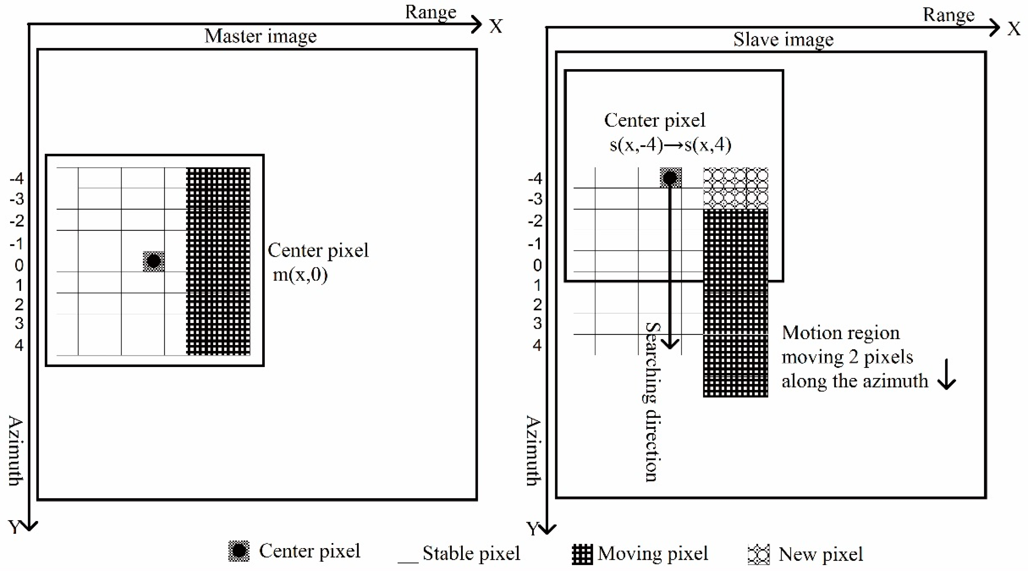
2.2. The Proposed Polarimetric Tracking Algorithm

A fully PolSAR system acquires four-channel images in the horizontal (H) and vertical (V) polarization basis. Then, the observed scattering matrix can be expressed as a 4-D polarimetric vector $\overrightarrow{K}={\left(S_{HH},S_{HV},S_{VH},S_{VV}\right)}^T$ [34]. For a monostatic backscattering system and a reciprocal target, the scattering matrix is symmetric; that is, $S_{HV}=S_{VH}$. Then, the 4-D scattering vector can be reduced to a 3-D polarimetric vector $\overrightarrow{K}={\left[S_{HH},\sqrt{2}{S}_{HV},S_{VV}\right]}^T$ [35].

Matching algorithms are based upon an assumption that the matched point and the reference point have similar characteristics. However, traditional single channel SAR images only have very limited information for reference in each pixel, so matching algorithms will use the statistical properties of the neighboring pixels to select tie-points. Compared with the single polarization SAR image, the fully polarimetric SAR image has more information contained in one pixel, which can better represent the scattering mechanisms of the targets. Thus, for PolSAR image registration, we can assume that the matched pixel and the reference pixel have the same polarimetric scattering mechanisms. As PolSAR is sensitive to the structure and orientation of the targets, many different types of target decomposition methods have been widely used to analyze the polarimetric scattering mechanisms of the targets [36,37,38,39,40]. For example, the Pauli decomposition—a widely used coherent target decomposition method for the PolSAR images—decomposes the target into three different basic scattering mechanisms: the surface or odd-bounce contributions ($(S_{HH}+S_{VV})/\sqrt{2}$), the double-bounce or even-bounce contributions ($(S_{HH}-S_{VV})/\sqrt{2}$), and the diffuse (volume) contributions ($\sqrt{2}{S}_{HV}$, in the monostatic case, where $S_{HV}=S_{VH}$). Surface contributions are mainly from point scatterers, flat surface, or trihedral corner reflectors. The double-bounce contributions are mainly from dihedral structures like ground–wall or ground–trunk. The diffuse (volume) contributions correspond to the statistical distributed scatterers like the forest canopy. After vectorization, the target’s Pauli decomposition vector can be written as in Equation (2).

$${\overrightarrow{K}}_p={\left[\begin{array}{ccc}(S_{HH}+S_{VV})/\sqrt{2},& (S_{HH}-S_{VV})/\sqrt{2},& \sqrt{2}{S}_{HV}\end{array}\right]}^T$$

(2)

According to the basic assumption mentioned above, we use the normalized inner product (NIP) of the two temporal PolSAR Pauli scattering vectors ${\overrightarrow{K}}_p^1$ and ${\overrightarrow{K}}_p^2$ for each image pixel as the criteria for matching.

$$\mathsf{\delta }=\frac{\left|{\overrightarrow{K}}_p^1\times {\overrightarrow{K}}_p^2\right|}{\Vert {\overrightarrow{K}}_p^1\Vert \times \Vert {\overrightarrow{K}}_p^2\Vert }$$

(3)

The normalized inner product $\mathsf{\delta }\in [0,1]$ measures how well the vectors ${\overrightarrow{K}}_p^1$ and ${\overrightarrow{K}}_p^2$ align linearly. When $\mathsf{\delta }=1$, the two scattering vectors are perfectly aligned or are linearly correlated. Conversely, when $\mathsf{\delta }=0$, the two scattering vectors are orthogonal, which means they are totally uncorrelated. For the two calibrated PolSAR data with the same acquiring conditions, amplitudes of each polarization channel for the same target are thought to be the same or similar. In this case, the NIP can be used to evaluate the similarity between two scattering vectors [41]. As PolSAR images are also affected by noise, we use the mean value $\langle \mathsf{\delta }\rangle$ of the polarimetric normalized inner product (PolNIP) of the neighboring pixels as the final correlation value. Like the traditional NCC method, offsets between the master and slave polarimetric SAR images are estimated by the location of the peak in the PolNIP matrix. Finally, the interpolation around the peak of the PolNIP matrix is used to achieve sub-pixel offsets.

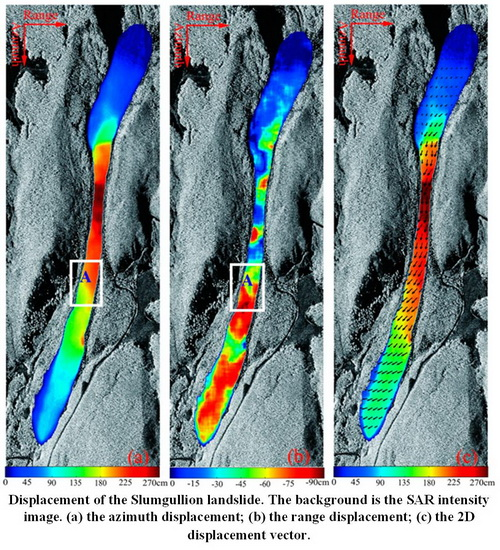
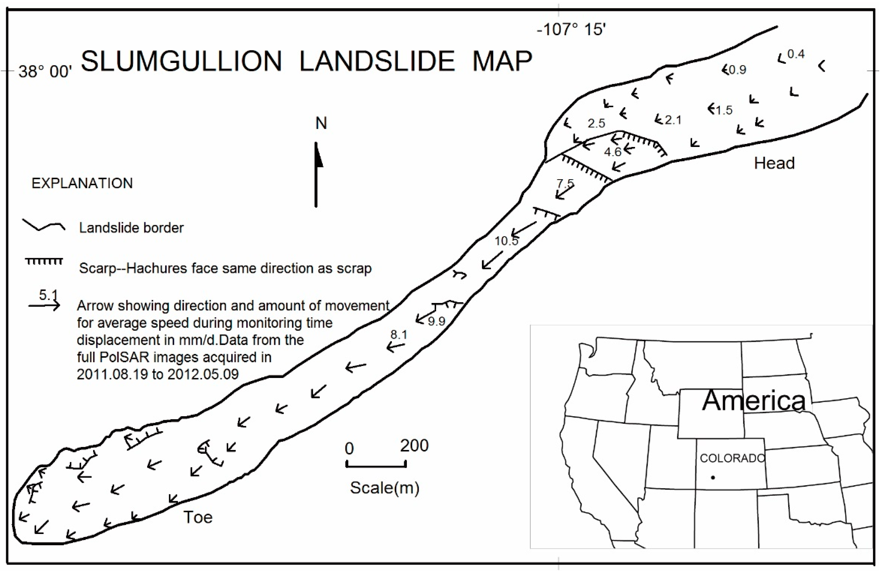
3. Study Area and Experimental Results

In order to validate the proposed method, two L-band fully PolSAR images acquired by the Jet Propulsion Laboratory’s Uninhabited Aerial Vehicle Synthetic Aperture Radar (UAVSAR) system are selected. These images cover the Slumgullion landslide (37°59′30″ N, 107°15′25″ W) located in the San Juan Mountains of Colorado, USA. It is reported that the Slumgullion landslide has been moving continually for over 300 years. It is one of the most famous landslides and is an Area of Critical Environmental Concern (ACEC) of USA. Its active part is about 3.9 km long [42], with widths ranging from 100 m to 500 m. The ground surface elevation along the landslide is between 2750 m and 3650 m [43,44]. A number of studies and experiments have been carried out relating to this area. Many scientists have made efforts to analyze its motion characteristics and inner mechanism. Milillo, etc. 2014 [45] used the COSMO-SkyMed Spotlight interferometry with a data acquisition interval of 24 h to inverse the Slumgullion landslide motion. In recent years, more and more fully polarimetric SAR data have been acquired by spaceborne and airborne SAR systems. The increasing polarimetric information provides opportunities to improve the accuracy of displacement estimation.

The two UAVSAR PolSAR images were acquired on 19 August 2011 and 9 May 2012, respectively, with an interval of 264 days.

Table 1. Detailed information of the UAVSAR polarimetric synthetic aperture radar (PolSAR) datasets.

Acquired Time	Polarization	Pixel Spacing (Azimuth)	Pixel Spacing (Range)	Wavelength
2011-08-19	HH, HV, VH, and VV	0.60 m	1.67 m	23.8 cm
2012-05-09	HH, HV, VH, and VV	0.60 m	1.67 m	23.8 cm

lists their detailed information. According to the former GPS surveying results, the maximum displacement in the neck area of the Slumgullion landslide can reach about three meters during the time interval of data acquisition. In this case, it is impossible for the traditional D-InSAR method to estimate the landslide displacement, because the displacement exceeds the maximum detectable deformation gradient of the D-InSAR method.

The azimuth displacement in Figure 1a shows that there is an obvious movement along the Slumgullion landslide, especially in its active part. The Slumgullion landslide can be simply divided into three main parts: the upper part, the hopper and neck area, and the lower part. The upper part indicates normal faults and tension cracks [44]. For the hopper and neck area, the elevation decreases sharply. The lower part indicates thrust faults [44]. Due to the complex fault movement inside the Slumgullion landslide, the range displacement (Figure 1b) shows more complex characteristics. Figure 1c shows the 2D displacement vectors composed of the azimuth and range displacement in Figure 1a,b. The displacement vector image presents the detailed information of the moving direction and scale. Based on Figure 1, we produce a simplified interpretive map of the Slumgullion landslide, as shown in Figure 2.

During the time interval between these two PolSAR images, the head of the Slumgullion landslide slid with an average rate of 1.6–2.1 mm/d. For the hopper and neck area—the narrowest part of the landslide, which looks like a funnel-shaped stretch [44]—the sliding rate reaches the maximum 10.1–10.9 mm/d. As described in reference [42], the monitoring site (located in the hopper and neck area) had an average velocity of 10 mm/d during the period of 12 August 2004–4 June 2006. The landslide then grows wider and slides more slowly downward. The average displacement rate for this area is 4.0–5.0 mm/d. More detailed landslide geological interpretations can be found in [42,43,44].

4. Discussion

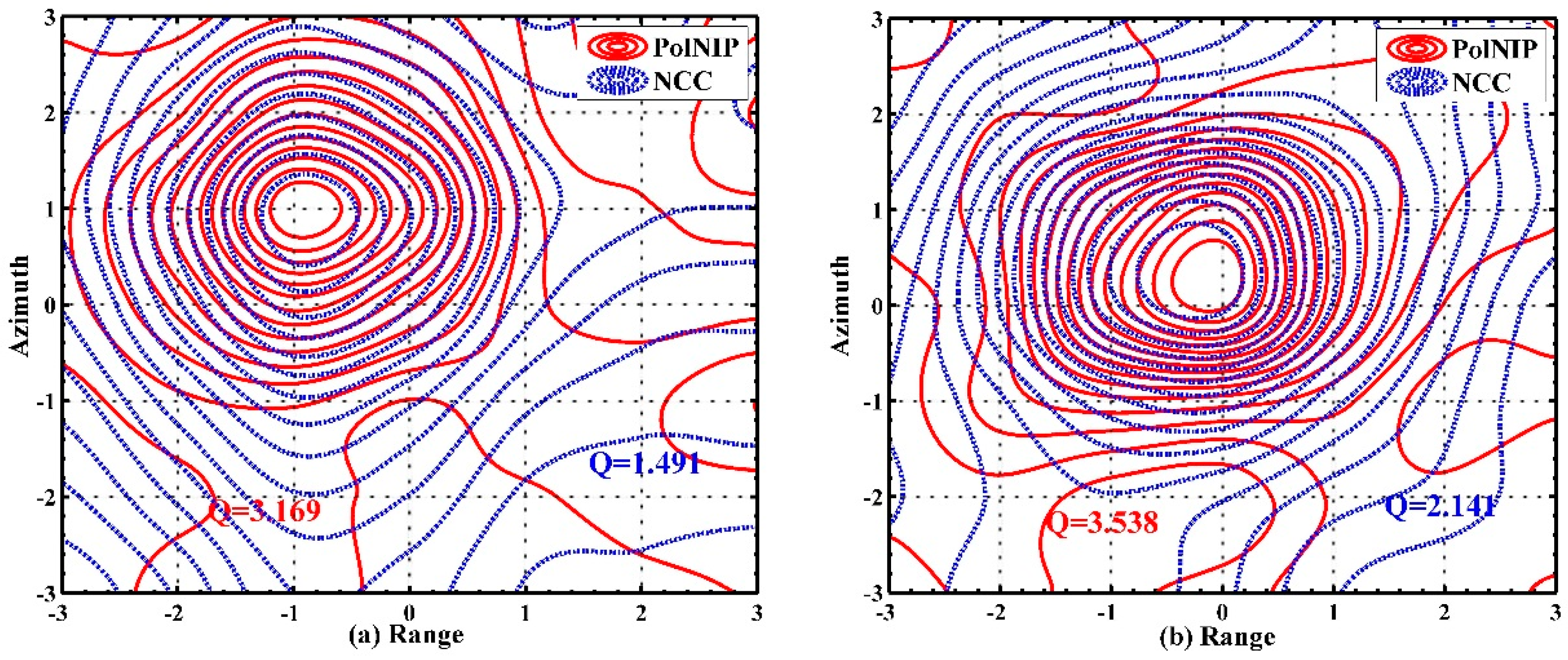
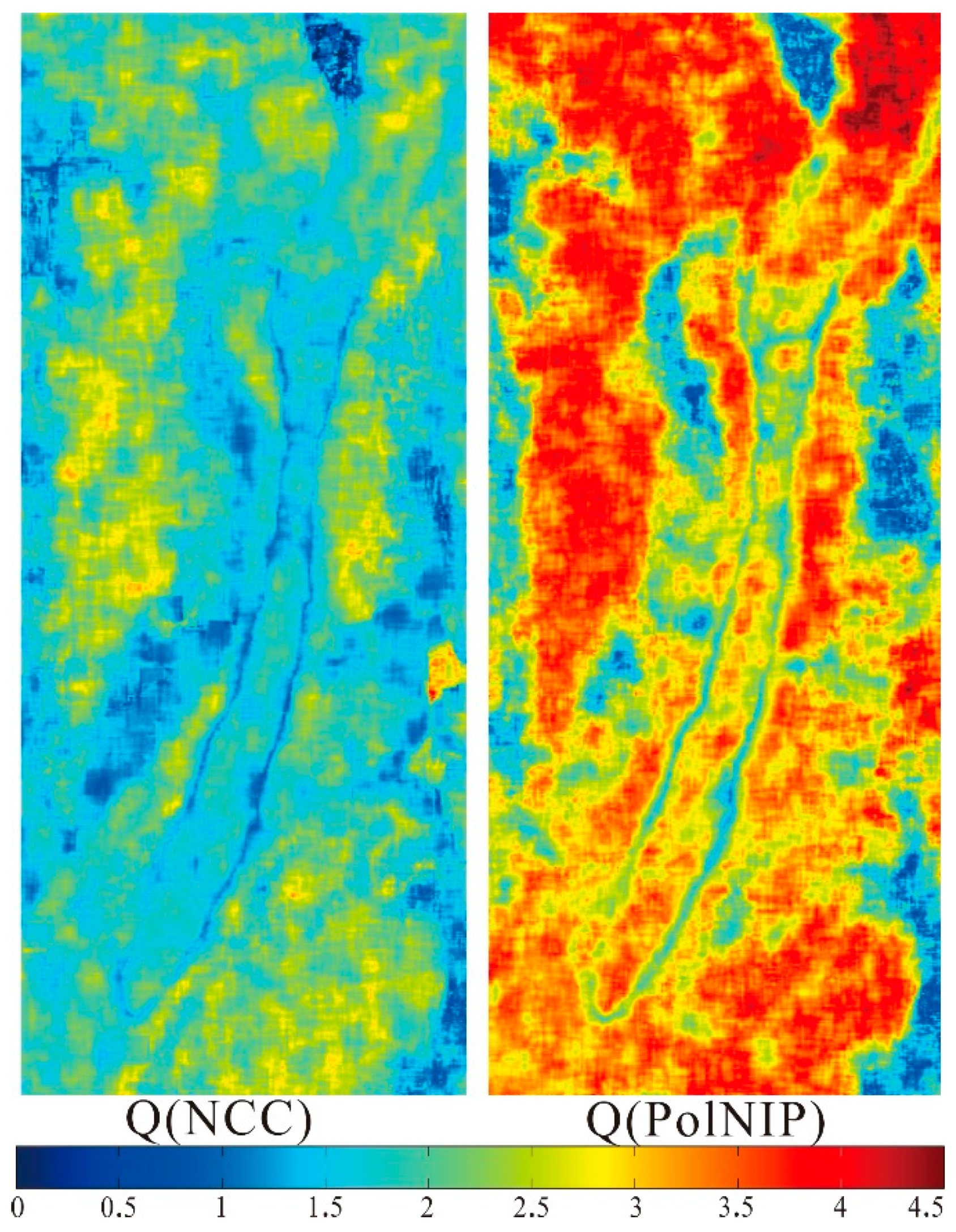
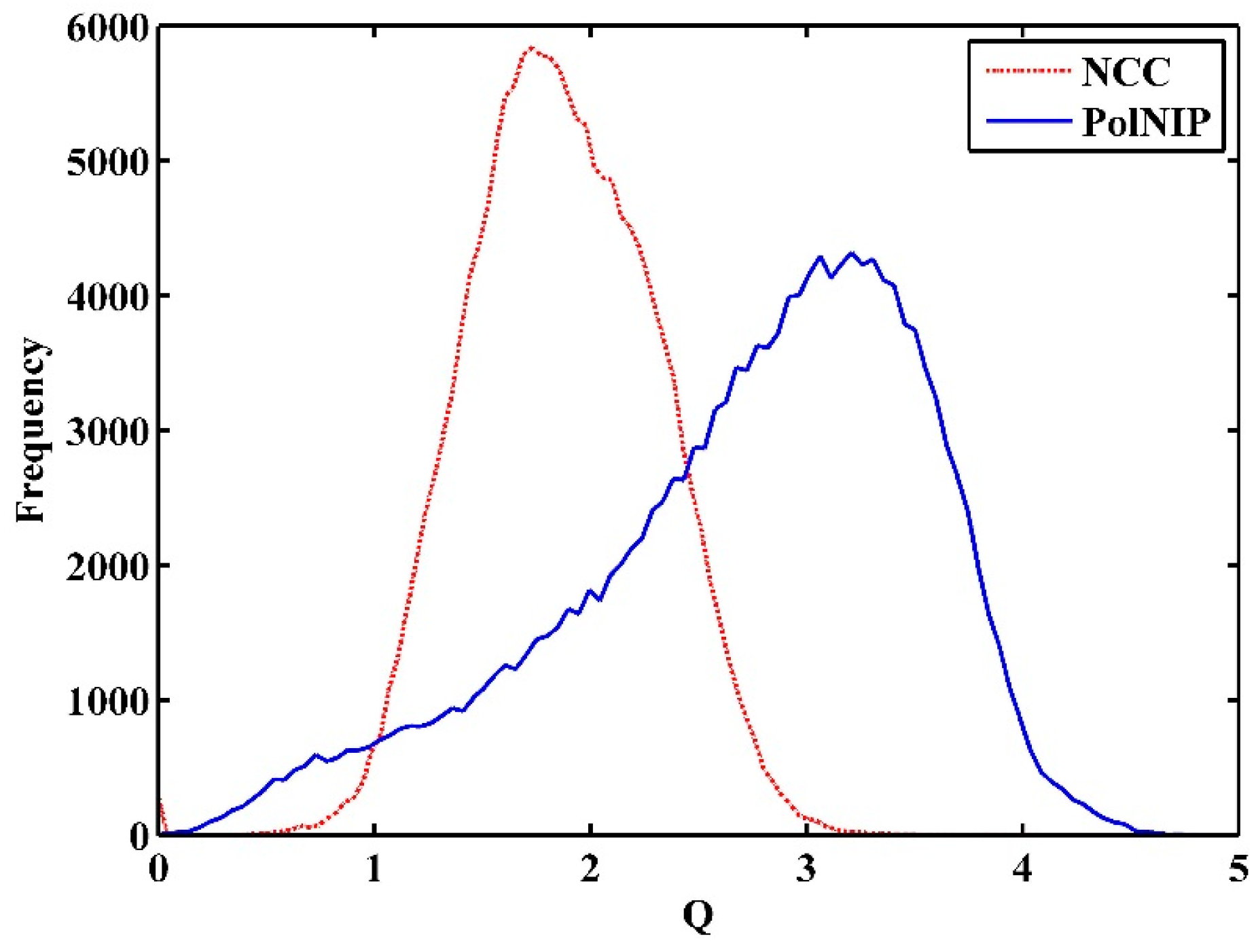
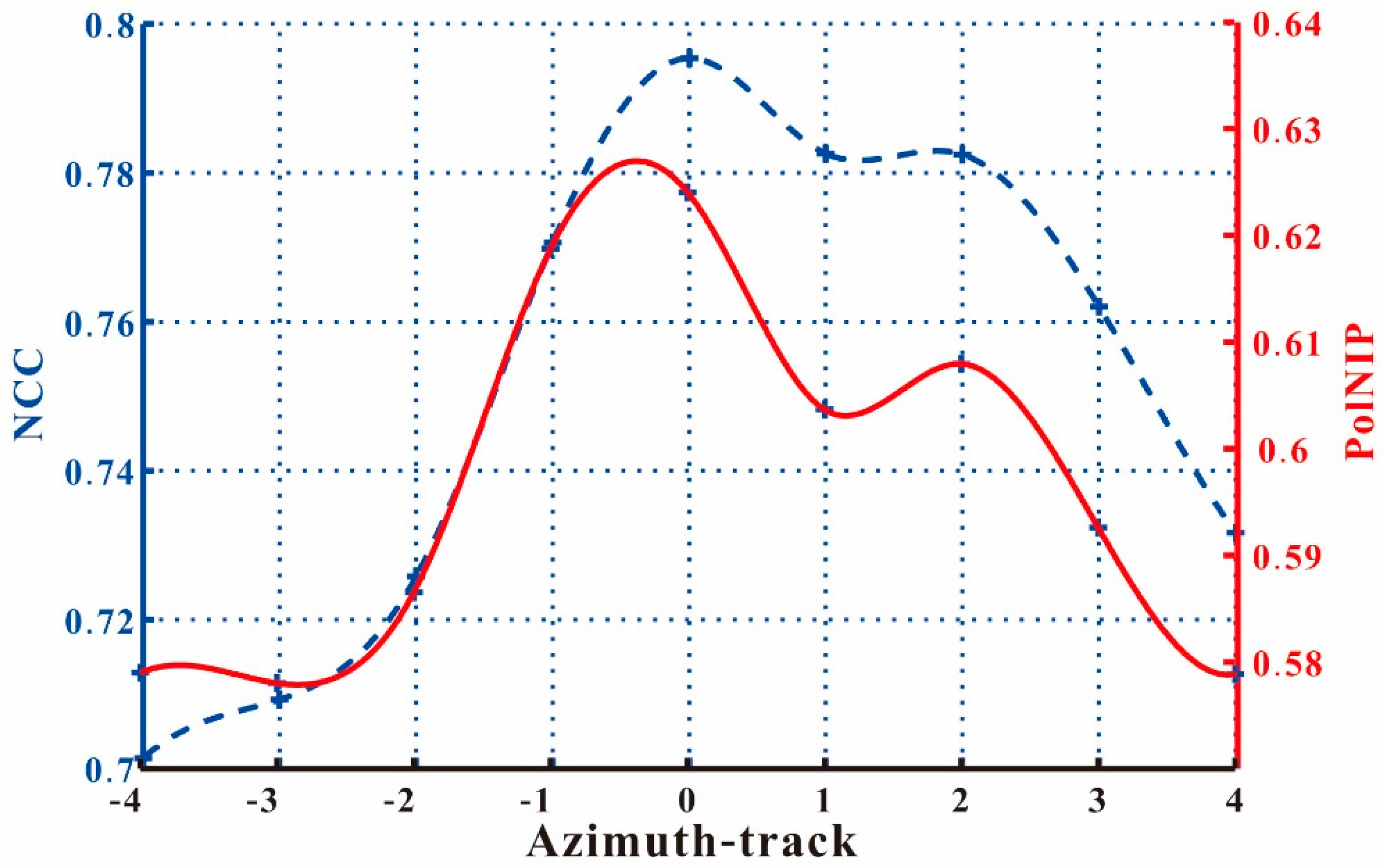
4.1. Performance of Sub-Pixel Estimation

To analyze the sub-pixel accuracy of the proposed method, we select the confidence measure Q introduced by Erten [31] as the criterion. The confidence measure Q is defined in Equation (4).

$$Q=\frac{\max (PolNIP)-mean(PolNIP)}{mean(PolNIP)-\min (PolNIP)}$$

(4)

The larger the Q value, the steeper the peak of PolNIP. In the sub-pixel matching method, the best matching position is found by maximizing the interpolation of the matching template’s correlation surface. Thus, the precision of the sub-pixel matching position is closely correlated to the steepness of the peak area around the estimated pixel. A larger Q value means more precise offset estimation. We select a pixel from the active area and the stable area to compare the matching performance of the NCC and the proposed PolNIP methods. Figure 3 shows the contour map of the interpolated correlation surface around the estimated pixel produced by the NCC and PolNIP methods.

In Figure 3, the contour maps of both the active area and the stable area produced by the PolNIP method are more concentrated around the peak than that of the NCC method. As we know, the denser the contour line, the steeper the peak, and the smaller the error of sub-pixel estimation. Therefore, compared with the traditional NCC method, the PolNIP method can improve the accuracy of sub-pixel matching with polarimetric information. Figure 4 shows the confidence measure (Q value) images of the whole experimental area obtained by the NCC and the PolNIP. We can find that, in either the moving area (along the Slumgullion landslide) or the stable area, the Q values of the PolNIP method are larger than that of the NCC method. Furthermore, we make two statistical histograms (Figure 5) of the Q values of these two methods. The histograms indicate that the PolNIP method has higher confidence.

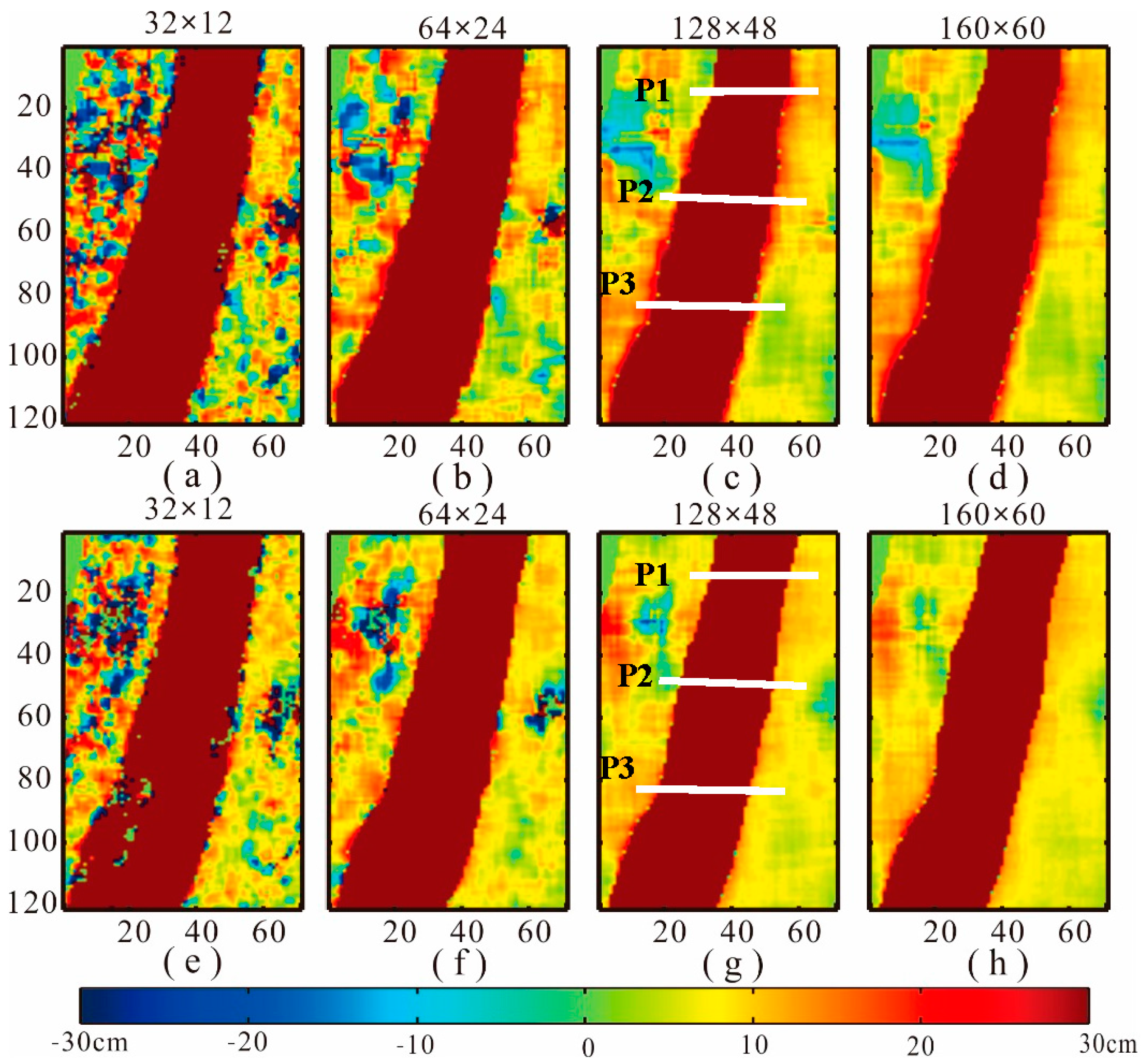
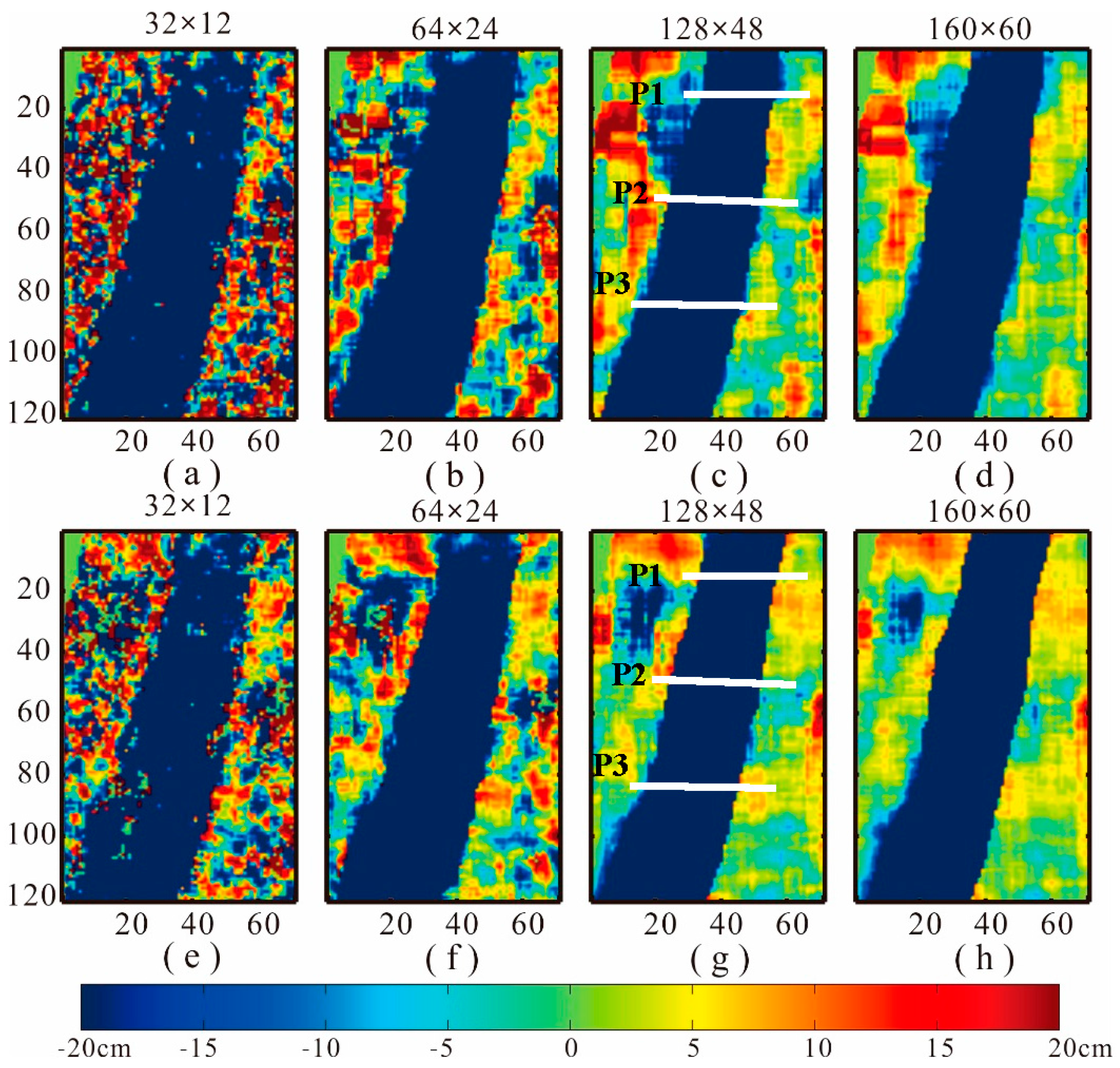
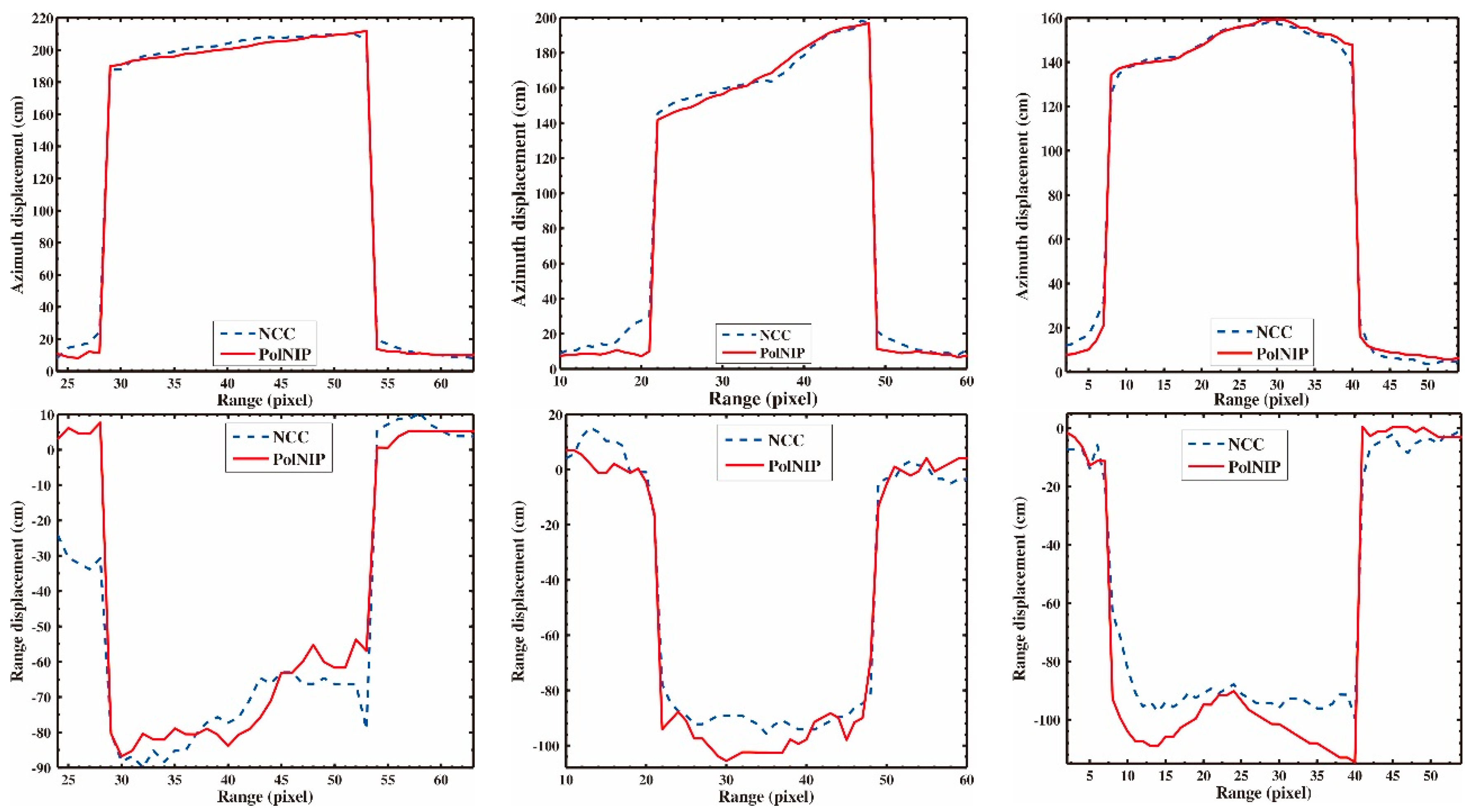
4.2. Performance of Displacement Estimation on Landslide Boundaries

The Slumgullion landslide has irregular boundaries, so the accurate estimation of the boundaries’ displacement is very important for the analysis of the structural features of the landslides. As the NCC uses a matching window (e.g., 32 × 32 pixels) to compute the normalized cross-correlation between two images, the matching window always contains both the moving area and the stable area around the landslide boundaries, affecting the estimation accuracy. Additionally, the size of the matching window significantly affects the correlation value and the precision of the displacement estimation. Figure 6 shows the estimated azimuth displacement maps produced by the NCC with HH channel data (top) and the PolNIP (bottom) method for the sub-area A in Figure 1 under different matching windows. We can see that as the matching window size increases, the estimated displacements become more accurate. The results of small matching windows contain more errors. However, results of large matching windows for the NCC method become blurred along the boundaries of the landslide, and the larger the matching window, the more blurred the displacement map. On the contrary, displacements at the boundaries obtained by the proposed PolNIP method only vary a little with increasing matching window size. Figure 7 shows the results of the range direction. Although the range resolution (1.67 m, as shown in Table 1) is much coarser than the azimuth resolution (0.60 m), we can see that the estimated range displacement of the NCC method is still more blurred than that of the PolNIP method. In addition, with the increasing window size, the estimated displacement variation tendency around the boundaries in the range direction agrees with that of the azimuth direction.

Figure 8 shows the azimuth (top) and range (bottom) displacement profiles of the NCC and the PolNIP methods with a matching window of size 128 × 48 pixels. Figure 8a indicates that the NCC and the PolNIP methods get relatively smooth curves of the azimuth displacement in the sliding area. However, around the landslide boundaries, the curve of the PolNIP method indicates more significant inflexion points than that of the NCC method. These inflexion points are the transition points between the stable area and the moving area. On the contrary, the curves of the range displacement present slight fluctuations in the sliding area. In addition, curves of the PolNIP method have significant inflexion points.

To figure out why the estimation results along the landslide boundaries obtained by the NCC method are more blurred, we plot a schematic diagram of the offsets estimation over an area containing stable and moving pixels, as shown in Figure 9. We assume the motion area in the slave image shifts two pixels along the azimuth direction relative to the master image. When the matching window in the slave image slides along the azimuth direction from s(x, −4) to s(x, 4) (relative to the center pixel in the master block), the fitted curve of the correlation value should have two peaks at s(x, 0) and s(x, 2), respectively. However, as shown in Figure 10, the normalized cross-correlation value of the NCC method is ambiguous for the peak of s(x, 2), which affects the sub-pixel accuracy offsets estimation. On the contrary, the proposed PolNIP method can get two peaks (as shown in Figure 10)—s(x, 0) and s(x, 2), respectively. The reason is that the adjacent pixels’ NCC value vary slightly due to similar intensity within the matching windows. In this case, it is not beneficial for offsets estimation of landslide boundary area. However, when the matching window slides one pixel for the PolNIP method, the polarimetric similarity for all pairs of temporal pixels’ Pauli scattering vectors may dramatically change. Then, the adjacent pixels’ PolNIP values have larger difference, which is beneficial for the location of a local peak for the fitted curve.

5. Conclusions

Based on the assumption that different ground objects can be distinguished by their polarimetric scattering properties, a new correlation measure based on fully PolSAR images for offset tracking method has been proposed for landslide displacement estimation. We apply it to the Slumgullion landslide displacement monitoring. The results show that from 19 August 2011 to 9 May 2012, the sliding velocity in different parts of the Slumgullion landslide ranged between 1.6–10.9 mm/d, which is consistent with former publications [42,43,44,46]. Compared with in-situ and GPS observations in the former publications, the landslide displacement maps produced by the proposed method have higher spatial resolution, which is beneficial for geologists in interpreting the formation activity of the Slumgullion landslide.

The proposed method has been evaluated on two aspects. One is the performance analysis on sub-pixel displacement estimation. A confidence measure (Q) was used to estimate the quality of the sub-pixel estimation. The value of Q calculated by the proposed method is about twice that of the NCC method. The other aspect is the performance analysis of displacement estimation on landslide boundaries. The matching window of the NCC method always contains both moving area and stable area around the landslide boundaries, which affects the displacement estimation accuracy. In addition, with the increasing size of matching windows, the azimuth and range displacements at the landslide boundaries estimated by the NCC method become more blurred. This means that the matching windows contain some areas with different moving characteristics, especially for the landslide boundaries. However, the proposed PolNIP method uses each pixel’s polarimetric information to partly reduce the effect of hybrid moving characteristics within the matching windows. The results of the proposed PolNIP method contain more detailed displacement information about the landslide boundaries. However, like the NCC method, the performance of the PolNIP method also depends on image resolution. In our experiments, we use high resolution PolSAR data, which makes it possible to use offset tracking method for monitoring of the landslide displacement. For medium resolution SAR data (e.g., Sentinel-1), the method will not deliver comparable results.

References

1. Dai, F.C.; Lee, C.F.; Ngai, Y.Y. Landslide risk assessment and management: An overview. Eng. Geol. 2002, 64, 65–87. [Google Scholar] [CrossRef]
2. Guzzetti, F.; Carrara, A.; Cardinali, M.; Reichenbach, P. Landslide hazard evaluation: A review of current techniques and their application in a multi-scale study, Central Italy. Geomorphology 1999, 31, 181–216. [Google Scholar] [CrossRef]
3. Varnes, D.J. Landslide Hazard Zonation: A Review of Principles and Practice; United Nations Educational Scientific And cultural Organization (UNESCO) Natural Hazards Press: Paris, France, 1984. [Google Scholar]
4. Scaioni, M.; Longoni, L.; Melillo, V.; Papini, M. Remote sensing for landslide investigations: An overview of recent achievements and perspectives. Remote Sens. 2014, 6, 9600–9652. [Google Scholar] [CrossRef]
5. Delacourt, C.; Allemand, P.; Casson, B.; Vadon, H. Velocity field of the “La Clapière” landslide measured by the correlation of aerial and QuickBird satellite images. Geophys. Res. Lett. 2004, 31, L15619. [Google Scholar] [CrossRef]
6. Rosen, P.A.; Hensley, S.; Joughin, I.R.; Madsen, S.N.; Rodriguez, E.; Goldstein, R.M. Synthetic aperture radar interferometry. Proc. IEEE 2000, 88, 333–382. [Google Scholar] [CrossRef]
7. Crosetto, M.; Gili, J.A.; Monserrat, O.; Cuevas-González, M.; Corominas, J.; Serral, D. Interferometric SAR monitoring of the Vallcebre landslide (Spain) using corner reflectors. Natl. Hazards Earth Syst. Sci. 2013, 13, 923–933. [Google Scholar] [CrossRef]
8. Ao, M.; Wang, C.; Xie, R.; Zhang, X.; Hu, J.; Du, Y.; Li, Z.; Zhu, J.; Dai, W.; Kuang, C. Monitoring the land subsidence with persistent scatterer interferometry in Nansha District, Guangdong, China. Natl. Hazards 2015, 75, 2947–2964. [Google Scholar] [CrossRef]
9. Berardino, P.; Fornaro, G.; Lanari, R.; Sansosti, E. A new algorithm for surface deformation monitoring based on small baseline differential SAR interferograms. IEEE Trans. Geosci. Remote Sens. 2002, 40, 2375–2383. [Google Scholar] [CrossRef]
10. Crosetto, M.; Castillo, M.; Arbiol, R. Urban subsidence monitoring using radar interferometry: Algorithms and validation. Photogramm. Eng. Remote Sens. 2003, 69, 775–783. [Google Scholar] [CrossRef]
11. Ferretti, A.; Prati, C.; Rocca, F. Nonlinear subsidence rate estimation using permanent scatterers in differential SAR interferometry. IEEE Trans. Geosci. Remote Sens. 2000, 38, 2202–2212. [Google Scholar] [CrossRef]
12. Sun, Q.; Zhang, L.; Ding, X.L.; Hu, J.; Li, Z.W.; Zhu, J.J. Slope deformation prior to Zhouqu, China landslide from InSAR time series analysis. Remote Sens. Environ. 2015, 156, 45–57. [Google Scholar] [CrossRef]
13. Hu, J.; Wang, Q.; Li, Z.; Zhao, R.; Sun, Q. Investigating the Ground Deformation and Source Model of the Yangbajing Geothermal Field in Tibet, China with the WLS InSAR Technique. Remote Sens. 2016, 8, 191. [Google Scholar] [CrossRef]
14. Pipia, L.; Fabregas, X.; Aguasca, A.; Lopez-Martinez, C.; Duque, S.; Mallorqui, J.J.; Marturia, J. Polarimetric differential SAR interferometry: First results with ground-based measurements. IEEE Geosci. Remote Sens. Lett. 2009, 6, 167–171. [Google Scholar] [CrossRef]
15. Navarro-Sanchez, V.D.; Lopez-Sanchez, J.M.; Vicente-Guijalba, F. A contribution of polarimetry to satellite differential SAR interferometry: Increasing the number of pixel candidates. IEEE Geosci. Remote Sens. Lett. 2010, 7, 276. [Google Scholar] [CrossRef]
16. Navarro-Sanchez, V.D.; Lopez-Sanchez, J.M.; Ferro-Famil, L. Polarimetric approaches for persistent scatterers interferometry. IEEE Trans. Geosci. Remote Sens. 2014, 52, 1667–1676. [Google Scholar] [CrossRef]
17. Colesanti, C.; Wasowski, J. Investigating landslides with space-borne Synthetic Aperture Radar (SAR) interferometry. Eng. Geol. 2006, 88, 173–199. [Google Scholar] [CrossRef]
18. Gabriel, A.K.; Goldstein, R.M.; Zebker, H.A. Mapping small elevation changes over large areas: Differential radar interferometry. J. Geophys. Res. Solid Earth 1989, 94, 9183–9191. [Google Scholar] [CrossRef]
19. Bamler, R.; Eineder, M. Accuracy of differential shift estimation by correlation and split-bandwidth interferometry for wideband and delta-k sar systems. IEEE Geosci. Remote Sens. Lett. 2005, 2, 151–155. [Google Scholar] [CrossRef]
20. Casu, F.; Manconi, A.; Pepe, A.; Lanari, R. Deformation time-series generation in areas characterized by large displacement dynamics: The SAR amplitude pixel-offset SBAS technique. IEEE Trans. Geosci. Remote Sens. 2011, 49, 2752–2763. [Google Scholar] [CrossRef]
21. R. Scheiber, M.; Jager, P.; Prats-Iraola, F.; De Zan, D. Geudtner, Speckle tracking and interferometric processing of TerraSAR-X TOPS data for mapping nonstationary scenarios. IEEE J. Sel. Topics Appl. Earth Observ. Remote Sens. 2015, 8, 1709–1720. [Google Scholar] [CrossRef]
22. Wegmuller, U.; Werner, C.; Strozzi, T.; Wiesmann, A. Ionospheric electron concentration effects on SAR and INSAR. In Proceedings of the 2006 IEEE International Symposium on Geoscience and Remote Sensing, Denver, CO, USA, 31 July 2006–4 August 2006; pp. 3731–3734.
23. Li, J.; Li, Z.; Wang, C.; Zhu, J.; Ding, X. Using SAR offset-tracking approach to estimate surface motion of the South Inylchek Glacier in Tianshan. Chin. J. Geophys. Chin. Ed. 2013, 56, 1226–1236. (In Chinese) [Google Scholar]
24. Debella-Gilo, M.; Kääb, A. Sub-pixel precision image matching for measuring surface displacements on mass movements using normalized cross-correlation. Remote Sens. Environ. 2011, 115, 130–142. [Google Scholar] [CrossRef]
25. Lowry, B.; Gomez, F.; Zhou, W.; Mooney, M.A.; Held, B.; Grasmick, J. High resolution displacement monitoring of a slow velocity landslide using ground based radar interferometry. Eng. Geol. 2013, 166, 160–169. [Google Scholar] [CrossRef]
26. Zitova, B.; Flusser, J. Image registration methods: A survey. Image Vis. Comput. 2003, 21, 977–1000. [Google Scholar] [CrossRef]
27. Fielding, E.J.; Lundgren, P.R.; Taymaz, T.; Yolsal-Çevikbilen, S.; Owen, S.E. Fault-Slip source models for the 2011 M 7.1 Van Earthquake in Turkey from SAR Interferometry, Pixel Offset Tracking, GPS, and Seismic Waveform Analysis. Seismol. Res. Lett. 2013, 84, 579–593. [Google Scholar] [CrossRef]
28. Feng, G.; Li, Z.; Shan, X.; Zhang, L.; Zhang, G.; Zhu, J. Geodetic model of the 2015 April 25 Mw 7.8 Gorkha Nepal Earthquake and Mw 7.3 aftershock estimated from InSAR and GPS data. Geophys. J. Int. 2015, 203, 896–900. [Google Scholar] [CrossRef]
29. Wang, T.; Wei, S.; Jónsson, S. Coseismic displacements from SAR image offsets between different satellite sensors: Application to the 2001 Bhuj (India) earthquake. Geophys. Res. Lett. 2015, 42, 7022–7030. [Google Scholar] [CrossRef]
30. Wang, T.; Jónsson, S. Improved SAR amplitude image offset measurements for deriving three-dimensional coseismic displacements. IEEE J. Sel. Topics Appl. Earth Observ. Remote Sens. 2015, 8, 3271–3278. [Google Scholar] [CrossRef]
31. Erten, E. Glacier velocity estimation by means of a polarimetric similarity measure. IEEE Trans. Geosci. Remote Sens. 2013, 51, 3319–3327. [Google Scholar] [CrossRef]
32. Erten, E.; Reigber, A.; Hellwich, O.; Prats, P. Glacier velocity monitoring by maximum likelihood texture tracking. IEEE Trans. Geosci. Remote Sens. 2009, 47, 394–405. [Google Scholar] [CrossRef]
33. Hii, A.J.H.; Hann, C.E.; Chase, J.G.; Van Houten, E.E.W. Fast normalized cross-correlation for motion tracking using basis functions. Comput. Methods Programs Biomed. 2006, 82, 144–156. [Google Scholar] [CrossRef] [PubMed]
34. Lee, J.S.; Pottier, E. Polarimetric Radar Imaging: From Basics to Applications; Francis Group Raton (CRC) Press: Boca Raton, FL, USA, 2009. [Google Scholar]
35. Cloude, S.R. Polarisation: Applications in Remote Sensing; Oxford University Press: Oxford, UK, 2009. [Google Scholar]
36. Cameron, W.L.; Leung, L.K. Feature motivated polarization scattering matrix decomposition. In Proceedings of the IEEE 1990 International Radar Conference, Arlington, VA, USA, 7–10 May 1990; pp. 549–557.
37. Krogager, E. New decomposition of the radar target scattering matrix. Electr. Lett. 1990, 26, 1525–1527. [Google Scholar] [CrossRef]
38. Freeman, A.; Durden, S.L. A three-component scattering model for polarimetric SAR data. IEEE Trans. Geosci. Remote Sens. 1998, 36, 963–973. [Google Scholar] [CrossRef]
39. Cloude, S.R.; Pottier, E. An entropy based classification scheme for land applications of polarimetric SAR. IEEE Trans. Geosci. Remote Sens. 1997, 35, 68–78. [Google Scholar] [CrossRef]
40. Yamaguchi, Y.; Moriyama, T.; Ishido, M.; Yamada, H. Four-component scattering model for polarimetric SAR image decomposition. IEEE Trans. Geosci. Remote Sens. 2005, 43, 1699–1706. [Google Scholar] [CrossRef]
41. Yang, J.; Peng, Y.N.; Lin, S.M. Similarity between two scattering matrices. Electr. Lett. 2001, 37, 1. [Google Scholar] [CrossRef]
42. Schulz, W.H.; McKenna, J.P.; Biavati, G.; Kibler, J.D. Characteristics of Slumgullion landslide inferred from subsurface exploration, in-situ and laboratory testing, and monitoring. In Proceedings of the 1st North American Landslide Conference, Vail, CO, USA, 3–10 June 2007; pp. 3–8.
43. Coe, J.A.; Ellis, W.L.; Godt, J.W.; Savage, W.Z.; Savage, J.E.; Michael, J.A.; Debray, S. Seasonal movement of the Slumgullion landslide determined from Global Positioning System surveys and field instrumentation, July 1998–March 2002. Eng. Geol. 2003, 68, 67–101. [Google Scholar] [CrossRef]
44. Fleming, R.W.; Baum, R.L.; Giardino, M. Map and Description of the Active Part of the Slumgullion Landslide, Hinsdale County, Colorado; US Department of the Interior, US Geological Survey: Denver, CO, USA, 1999.
45. Milillo, P.; Fielding, E.J.; Shulz, W.H.; Delbridge, B.; Burgmann, R. COSMO-SkyMed spotlight interferometry over rural areas: The Slumgullion landslide in Colorado, USA. IEEE J. Sel. Top. Appl. Earth Observ. Remote Sens. 2014, 7, 2919–2926. [Google Scholar] [CrossRef]
46. Parise, M.A.; Coe, J.A.; Savage, W.Z.; Varnes, D.J. The Slumgullion landslide (southwestern Colorado, USA): Investigation and monitoring. In Proceedings of the International Conference FLOWS, Sorrento, Italy, 11–13 May 2003.
Figure 1. Displacement of the Slumgullion landslide. The background is the SAR intensity image. (a) the azimuth displacement; (b) the range displacement; (c) the 2D displacement vector.
Remotesensing 08 00624 g001
Figure 2. Simplified interpretive map of the Slumgullion landslide map, produced based on the the 2D displacement vector image Figure 1c.
Remotesensing 08 00624 g002
Figure 3. Contour map of the correlation (a) active area; (b) stable area.
Remotesensing 08 00624 g003
Figure 4. Quality measure Q of the normalized cross-correlation (NCC) and the polarimetric normalized inner product (PolNIP) methods. In reference to the SAR intensity image in Figure 1, the quality maps show that the confidence in the shadow or water areas (the dark area in Figure 1) is much lower than that of the other areas.
Remotesensing 08 00624 g004
Figure 5. Histograms of the quality measure Q of the NCC and the PolNIP methods.
Remotesensing 08 00624 g005
Figure 6. Estimated azimuth displacement maps of the white rectangle A in Figure 1. The displacement maps were computed by the NCC (ad) and the proposed PolNIP (eh) methods under different sizes of windows, such as 32 × 12, 64 × 24, 128 × 48, and 160 × 60 pixels. To highlight the difference of offset estimation with these two methods, we readjust the display range to [−30, 30] cm.
Remotesensing 08 00624 g006
Figure 7. Estimated range displacement maps of the white rectangle A in Figure 1. The displacement maps were computed by NCC (ad) and the proposed PolNIP (eh) methods under different sizes of windows, such as 32 × 12, 64 × 24, 128 × 48, and 160 × 60 pixels. We also readjust the display range to [−20, 20] cm to highlight the difference.
Remotesensing 08 00624 g007
Figure 8. Azimuth (top) and range (bottom) displacement profiles of the white lines (P1, P2, and P3) in Figure 6c,g and Figure 7c,g with a estimation window of size 128 × 48 pixels. Blue dashed lines and red solid lines indicate the displacement profiles of the NCC and the PolNIP methods, respectively.
Remotesensing 08 00624 g008
Figure 9. Schematic diagram for the offsets estimation of the NCC method over an area containing stable and moving pixels.
Remotesensing 08 00624 g009
Figure 10. Fitted curve of the correlation value of the NCC method (the blue dashed line) and the PolNIP method (the red solid line).
Remotesensing 08 00624 g010