Article

Spectral-Spatial Classification of Hyperspectral Images Using Joint Bilateral Filter and Graph Cut Based Model

Institute of Geophysics and Geomatics, China University of Geosciences, Wuhan 430074, China
*
Author to whom correspondence should be addressed.
Submission received: 21 July 2016 / Revised: 19 August 2016 / Accepted: 5 September 2016 / Published: 11 September 2016

Abstract

:
Hyperspectral image classification can be achieved by modeling an energy minimization problem on a graph of image pixels. In this paper, an effective spectral-spatial classification method for hyperspectral images based on joint bilateral filtering (JBF) and graph cut segmentation is proposed. In this method, a novel technique for labeling regions obtained by the spectral-spatial segmentation process is presented. Our method includes the following steps. First, the probabilistic support vector machines (SVM) classifier is used to estimate probabilities belonging to each information class. Second, an extended JBF is employed to perform image smoothing on the probability maps. By using our JBF process, salt-and-pepper classification noise in homogeneous regions can be effectively smoothed out while object boundaries in the original image are better preserved as well. Third, a sequence of modified bi-labeling graph cut models is constructed for each information class to extract the desirable object belonging to the corresponding class from the smoothed probability maps. Finally, a classification map is achieved by merging the segmentation maps obtained in the last step using a simple and effective rule. Experimental results based on three benchmark airborne hyperspectral datasets with different resolutions and contexts demonstrate that our method can achieve 8.56%–13.68% higher overall accuracies than the pixel-wise SVM classifier. The performance of our method was further compared to several classical hyperspectral image classification methods using objective quantitative measures and a visual qualitative evaluation.

Graphical Abstract

1. Introduction

Hyperspectral images can provide much valuable information due to high spectral and spatial resolutions. Therefore, hyperspectral imaging techniques have been widely used for various applications. However, a large number of spectral channels, the high spectral redundancy, spectral and spatial variabilities, together with limited ground truth data, present challenges to hyperspectral image analysis and classification. As a consequence, the traditional multispectral image classifiers are not suitable to classification of hyperspectral images. Many contributions have been devoted in the last decade to improving classification accuracies of hyperspectral images [1,2]. One of the most widely used techniques is SVM [3,4], which can demonstrate preferable performance with a limited number of training samples. However, these pixel-wise techniques classify hyperspectral images only using spectral information, without considering spatial dependencies, which limits their applicability.
Recently, several achievements were proposed for combining spectral and spatial information of hyperspectral images in the classification process. For instance, we can obtain more accurate classification maps by a pixel-wise classifier using spatial contextual information such as grey level co-occurrence matrix (GLCM) [5,6], extended morphological profiles (EMP) [7], pixel shape index [8], extended morphological attribute profile (EAP) [9], texture information based on Gabor filter [10,11], wavelet texture feature [12,13,14], etc. Another way for performing spectral-spatial classification was achieved by different segmentation techniques of watershed [15], mean shift [16,17], hierarchical segmentation [18,19], superpixel segmentation [20], extraction and classification of homogeneous objects [21], minimum spanning forest [22], fractal net evolution approach-based segmentation [6], etc. Apart from those efforts, some advanced spectral-spatial classification methods have been presented, by using multiple kernels learning [23] and generalized composite kernels [24], to integrate spatial features with spectral signatures.
In the spectral-spatial segmentation process, hyperspectral images are partitioned into homogeneous regions and all pixels in each region are assigned the same information class labels. To label these regions, two techniques are always employed [15]. The first one is to use a supervised classifier to directly classify these regions, which are considered as input vectors [25]. While the second one is to combine a pixel-wise classification map and a region-based segmentation map to obtain a final spectral-spatial classification map by using majority voting [15,22] or class labels of automatically selected markers [18]. If a maximum vote decision rule is used, the class label of each region is determined by the most frequent class in the same region according to the pixel-wise classification map; while if representative spectra in hyperspectral images are automatically extracted, the marker-based segmentation algorithm can be performed to obtain a segmentation map, in which class labels of those homogeneous regions are determined by that of markers obtained by a pixel-wise classifier.
It is well-known that many early vision problems can be naturally expressed in terms of energy minimization. However, interesting energies are often difficult to minimize because it always requires minimizing a non-convex function in a space with thousands of dimensions [26]. If the functions are formulated with a regularized form, the global minima of these functions can be efficiently solved using dynamic programming [27], which cannot solve energy functions in multidimensional settings. In the last decade, a novel energy minimization scheme has been presented based on graph cuts and its basic idea is to construct a specialized graph for the energy function to be minimized and the minimum cut on the graph can be effectively applied for minimizing the energy. Furthermore, the minimum cut can be computed very efficiently by max flow algorithms in graph theory. The advantages of modeling segmentation problems by means of graph theory are twofold: Firstly, mapping image elements onto a graph is an abstract way to build mathematically reasonable structures, in which relationships between entities can be measured. Secondly, the segmentation problem can be more flexible and very efficiently solved by the convenient tools from graph theory. Many intensive segmentation methods based on graph cuts have been presented, such as minimal cut, normalized cut, s/t graph cut, multi-labeling graph cut, interactive graph cut, etc. [28]. It is known that the hyperspectral image classification task can be solved by modeling an energy minimization problem on a graph of image pixels. In addition, both of spectral and spatial features in the image can be naturally utilized in the graph model. Therefore, spectral-spatial classification methods based on graph cuts have been developed. For instance, Yu et al. [29] proposed a multiscale graph cut based classification method, where region adjacency graph is employed to represent hyperspectral image in multiscale levels and the SVM classifier is used to classify multiscale context driven features; Tarabalka and Rana [30] proposed a spectral-spatial classification method based on a graph-cut-based model by computing an energy minimization problem on an image graph and using the graph-cut α-expansion approach to solve the problem; Ma et al. [31] proposed a graph-based learning semi-supervised method and a local-manifold-learning-based graph construction method; Bai et al. [32] employed a graph cut algorithm to solve the labeling problem on Markov random field (MRF), which was constructed on the image grid; Jia et al. [33] applied the graph cuts segmentation algorithm on the sparse-representation-based probability estimates of hyperspectral image to exploit spatial information; and Damodaran et al. [34] used the graph cut to minimize the MRF energy to gain the final classification map in the proposed dynamic classifier selection/dynamic ensemble selection method.
In this paper, we propose a novel spectral-spatial classification method for hyperspectral images based on JBF and graph cut segmentation. In this method, an alternative technique for labeling regions obtained by the spectral-spatial segmentation process is presented. Our method includes four main steps. First, the probabilistic SVM classifier is used to obtain class membership probability maps for each information class. Second, an extended JBF is employed to perform image smoothing on the probability maps. By using our JBF process, salt-and-pepper classification noise in homogeneous regions can be effectively smoothed out while object boundaries in the original image are better preserved as well. Third, a sequence of modified bi-labeling graph cut models is constructed for each information class to separate the desirable object (each class) belonging to the corresponding class from the smoothed probability maps. Finally, an ultimate spectral-spatial classification map is achieved by merging a sequence of the segmentation maps obtained in the last step using a simple rule. It should be noted that the proposed method is greatly different from the segmentation-based spectral-spatial classification methods mentioned above in terms of the strategy for labeling segments. Therefore, the major contribution of this work is to explore a novel framework to perform spatial-spectral classification of hyperspectral images.
The remainder of this paper is organized as follows: Section 2 reviews the techniques of bilateral filter and graph cut; Section 3 presents the proposed spectral-spatial classification of hyperspectral imagery; Section 4 describes the experimental results; Section 5 includes discussions of our method; and Section 6 states our concluding remarks.

2. Related Techniques

2.1. Bilateral Filter

The bilateral filter which was firstly proposed by Tomasi and Manduchi [35] is a classical edge-preserving smoothing technique. It is almost like a Gaussian filter, except that the bilateral filter is modulated by a function of the similarity between the central pixel (where the filter is applied) and its neighborhoods (that is used in blurring), and a function of the difference in intensity value with the neighborhoods as well. Let u denotes the input image and BF(u) represents its smoothed version by a bilateral filter applied to the image u, the classical bilateral filter is defined as follows:
B F ( u ) i = 1 W i j Ω G σ s ( i j ) G σ r ( u i u j ) u j
where the normalization term W i ensures that pixel weights sum to 1 and defined by:
W i = j Ω G σ s ( i j ) G σ r ( u i u j )
In Equation (1), i represents the pixel location at the center of the Gaussian kernel and j denotes the pixel location in the domain Ω which is a local window of size ( 2 n + 1 ) 2 , where n = 1 , 2 , , M . u j is the image intensity value at the jth pixel. i j means the L2 norm of ( i j ) . G σ s and G σ r denote the spatial and the range Gaussian kernels with standard deviation σ s and σ r , respectively. If intensity values of two adjacent pixels are very close, i.e., u i u j , it multiplies the Gaussian weight by something close to one, and hence it is equivalent to a Gaussian filter. In contrast, if the neighboring pixels have quite different intensity values, i.e., | u i u j | is very large, the Gaussian smoothing for this pixel is prohibited. Intuitively, this behavior yields the following result: Gaussian smoothing in homogeneous areas of the image, no filtering across object boundaries. The bilateral filter can effectively produce more pleasant results, because it avoids the introduction of blur between objects while removing noise in homogeneous areas. In addition, the bilateral filter can be adjusted by σ s and σ r , without an iterative manner.

2.2. Image Segmentation by Graph Cut

The graph cut algorithms have become very popular in image segmentation due to the fact that graph cut can provide a convenient language to encode simple local segmentation cues, together with a set of powerful computational mechanisms to extract global segmentation from those simple local pixel similarities. Moreover, graph cuts can be computed very conveniently by the efficient tools from graph theory [36].
(1) s/t graph cut
Let an undirected graph be denoted as G = ( V , E ) , with the set of vertices V corresponding to the pixels u in the image. Edges E of G occur between any two pixels ui and uj within a small distance of each other. An s/t graph in the graph cut model is a weighted directed graph with two identified nodes, i.e., the source s and the sink t. In this graph, E is composed of two types of edges: (i) every pair of neighborhood vertices, which correspond to all pixels in an image, is connected by an n-link; and (ii) the terminal nodes of s and t are connected to other vertices by t-links. The segmentation problem can be solved by partitioning the vertices of a graph G into two disjoint sets S and T by using an s/t cut, where s S , t T and S T = V , that minimizes the cost of the cut
c u t ( S , T ) = i S , j T a ( u i , u j )
where a ( , ) is the affinity function. If the cost of a cut of G is smaller than that of any other cut, the minimum cut can be obtained. As the Ford–Fulkerson theorem states [37], the maximum value of an s/t flow is equivalent to the minimum cost of an s/t cut. Therefore, the efficient max-flow/min-cut algorithm proposed by Boykov and Kolmogorov [38] can be utilized to generate the minimum cut for the s/t graph.
(2) s/t graph cut based segmentation
The s/t cut is well suited for two-class image segmentation [39]. For instance, pixels in an image can be represented by the vertices of the s/t graph and any neighborhood relationship between the pixels can be indicated by an edge. The partition problem can be regarded as assigning a label from the set L = { L i | i = 1 , 2 , , N } , where L i = { 0 , 1 } , to each pixel in the image, where 1 represents the label of “object” and 0 indicates the label of “background”. As a result, the globally optimal segmentation of image can be achieved by graph cuts. The energy functional, which can be minimized by the minimum cut in the s/t graph, is shown as follows [39,40]:
E ( L ) = B ( L ) + ω R ( L )
where R(L) denotes the regional term and can be defined as follows:
R ( L ) = i = 1 N R i ( L i )
The regional term measures penalties for assigning a pixel i to “object” and “background” and can be obtained by comparing the intensity of the ith pixel with a given intensity model (e.g., histogram) of the object and background. The other term on the right-hand side of Equation (4) is the boundary term and its definition is shown as follows
B ( L ) = ( i , j ) C B i , j ( L i , L j ) δ ( L i , L j )
where the ith and jth pixels are neighboring ones and C defines the neighborhoods of the ith pixel.
δ ( L i , L j ) = { 1 i f L i L j 0 otherwise .
The boundary term B(L) can be considered as a penalty for a dissimilarity between the ith and jth pixels. The penalty B i , j can be defined as a non-increasing function of distance between the ith and jth pixels and the corresponding distance can be measured using local gradient and its direction, Laplacian zero-crossing and other criteria. In addition, ω is a relative importance parameter to balance the two terms in Equation (4). As mentioned above, the minimized energy can be computed by the max-flow/min-cut algorithm Therefore, the energy minimization is converted into the graph cut problem. To obtain desirable segmentation results, weights of edges in the s/t graph are greatly significant.

3. Spectral-Spatial Classification Using Joint Bilateral Filter and Graph Cut Based Model

In this work, a spectral-spatial classification method of hyperspectral images based on joint bilateral filtering and class-specific graph cut segmentation, is proposed. A flow-chart of our classification method using the Indian Pines dataset as an example is summarized in Figure 1. First, a supervised probabilistic SVM classifier is applied to the original hyperspectral image to obtain class membership probability maps. Then, the SVM probability estimates are smoothed by an extended JBF, in which the original hyperspectral image is utilized as a guidance image for calculating range (photometric) weights. Next, a sequence of s/t cut energy functions are built for extracting each specific class from the smoothed probability maps. Finally, a simple and effective method is used to integrate all of the segmentation maps into a final classification map. In this section, the details of the proposed classification method are briefly introduced.

3.1. Probabilistic SVM Classification

Given an original B-band hyperspectral image which is composed of N pixel vectors U = { u i R B , i = 1 , 2 , , N } , where u i = { u i 1 , u i 2 , , u i B } . Information classes of interest in the image are defined as W = { w 1 , w 2 , , w K } , where K is the number of classes. In this work, the probabilistic SVM classifier is employed to perform the pixel-wise classification on the input hyperspectral image. To compute class membership probabilities, the pairwise coupling method is used by using the LIBSVM software [41,42]. The details on the SVM classifier and its application can be found in [4,43]. By applying the probabilistic SVM classifier to the original image, we can obtain following outputs:
(1)
A classification map, in which each pixel has a unique information class label;
(2)
Probability maps. Let P = { P k , k = 1 , 2 , , K } be the output probability maps and each pixel has a probability value, which indicates the probability belonging to the class of w k ( k = 1 , 2 , , K ), on the kth probability map P k = { p 1 k , p 2 k , , p N k } , where p i k is the probability value of the ith pixel.

3.2. Joint Bilateral Filter

As described in Section 2.1, the bilateral filter is a classical edge-preserving algorithm and has been widely used for various applications due to its high extendibility [44]. In this work, it is used for smoothing class membership probability maps. However, if this filter is directly applied to the probability maps, only class-specific features contained in the map are utilized, without taking spatial information between adjacent spectral signatures in hyperspectral imagery into account. Meanwhile, salt-and-pepper classification noise in the probability maps makes it difficult to accurately locate material boundaries, which is greatly significant for object extraction and recognition. Therefore, it is required for a probabilistic filter to preserve material boundaries while removing artifacts. To this end, an effective algorithm is presented to smooth the probability maps by employing the framework of bilateral filter. The technique of JBF was proposed by Petschnigg et al. [45] as an extension of the bilateral filter. In this work, we extend a JBF for probability maps while using the original hyperspectral image as a guide to compute the range weights G σ r , instead of the probability maps. For simplicity, the superscript k of p i k is omitted and the proposed filtering technique is defined as follows:
J B F ( P ) i = 1 W i j Ω G σ s ( i j ) G σ r ( | u i u j | ) p j
with
G σ s ( i j ) = e ( i j ) / 2 σ s 2
G σ r ( | u i u j | ) = e ( | u i u j | ) / 2 σ r 2
W i = j Ω G σ s ( i j ) G σ r ( | u i u j | )
where | u i u j | measures the dissimilarity between the ith and jth spectral vectors in the image and can be calculated using the Euclidean distance (ED), the spectral angle mapper (SAM) measure or the spectral information divergence (SID). In this work, the SAM measure is used as the dissimilarity measure in Equation (8) and is shown as follows:
| u i u j | SAM = arccos ( b = 1 N u i b u j b b = 1 N u i b 2 b = 1 N u j b 2 )
The proposed JBF is different from the standard bilateral filter in two aspects. First, it is performed on the obtained SVM class membership probability maps, instead of the original image. Second, the original image is adopted as a guide image because it can provide all valuable edge information. It can be observed in Equation (8) that both of spatial information and spectral features in hyperspectral imagery are combined in the proposed JBF. Consequently, the smoothed probability maps can provide more reliable information for further segmentation.

3.3. Class-Specific Graph-Cut (CS-GC) Method

In this subsection, the proposed spectral-spatial classification method for hyperspectral imagery based on a graph cut is carefully introduced. For clarification, the energy functional with respect to the probability map of p k ( k = 1 , 2 , , K ) is set as an example. In the s/t graph cut segmentation map achieved by our method, pixels belonging to the kth class are labeled as “object”, while the remaining pixels are assigned to “background”. In this way, pixels of each information class are extracted and labeled 1. The class-specific graph-cut method mainly includes three steps:
(1)
Construction of a class-specific graph-cut-based model;
(2)
The class-specific energy functional minimization; and
(3)
Image labeling based on graph cut Model.
(1) Construction of a class-specific graph-cut-based model
Let L k = { L 1 k , L 2 k , , L N k } be a set of class label of each pixel with respect to the kth class, where L i k = { 0 , 1 } , i = 1 , 2 , , N . If the ith pixel vector belongs to the kth information class, its class label is set to 1, i.e., L i k = 1 ; otherwise, this pixel vector belongs to the other classes with L i k = 0 . According to graph theory, we build a Gibbs energy functional for the kth class as follows:
E ( L k , p k , u ) = i = 1 N V ( L i k , p k ) + ω ( i , j ) C W i , j ( L i k , L j k , u )
where V ( L i k , p k ) is the data term in the energy functional and it is utilized to measure the fit of assigning label L k to the probability map p k . In this work, this term is defined using the smoothed probability maps as follows:
V ( L i k , p i k ) = { e x p ( p i k μ ) , L i k = 1 e x p ( 1 p i k 1 μ ) , L i k = 0
where μ ( 0 < μ 1 ) is a parameter to control the strength of the data term. The proposed graph cut based model is built based the competition between “object” and “background” and μ can be used to balance the two opponents. For instance, if p i k is larger than μ, then V ( 1 , p i k ) is greater than V ( 0 , p i k ) according to Equation (14), which means that the ith pixel vector may belong to the class of “object”. Otherwise, p i k is very small and the pixel vector is more likely to be classified as “background”. The smoothness term W ( L i k , L j k , u ) in Equation (13) is defined as follows:
V ( L k , u ) = ω ( i , j ) C exp ( β | u i u j | ) δ ( L i , L j )
where an eight-neighborhood system is employed in the proposed energy model, and | u i u j | can be computed according to Equation (12). ω is a parameter to control the weight of spatial smoothing. The parameter β is defined as described in [46] to be
β = ( 2 | u i u j | ) 1
where denotes expectation over an image sample.
(2) The class-specific energy functional minimization
Once the energy functional is defined, a set of “object” pixels belonging to the kth class can be extracted by estimating a global minimum of the energy functional:
L ^ k = arg min L k   E ( L k , p k , u )
The energy minimization can be solved by using the standard minimum cut algorithm proposed by Boykov and Jolly [39]. In this way, we build the proposed graph cut based model for each class and extract the corresponding “object” areas. As a consequence, a sequence of object extraction maps O = { o i R K , i = 1 , 2 , , N } , are obtained, where o i = ( o i 1 , o i 2 , , o i K ) .
(3) Image labeling based on graph cut Model
As mentioned in the first step, each of the segmentation maps is assigned two labels: 0 for background and 1 for the specific class. In this step, these maps are integrated into a final classification map. To this end, a simple and effective method, which is performed on these segmentation maps, is presented. For each pixel in the object extraction maps,
(i)
If the maximum value of its labels, i.e., max ( o i 1 , o i 2 , , o i K ) , is equal to 1 and the sum of its labels j = 1 K o i j is equal to 1 as well, the final class label of the ith pixel is set to 1; otherwise, the class label of this pixel is assigned to 0.
(ii)
If the class label of a pixel is 0, we assign this pixel a final information class label by performing classification based on the maximum probability.
Finally, the spectral-spatial classification map is obtained using our proposed CS-GC method with JBF.

3.4. Parallelizing Algorithms

The proposed methods are highly suitable for high-performance parallel computing because they can be divided into several image tasks, which can be naturally executed at multiple levels. In this subsection, we investigate the parallel implementation of the CS-GC model with the optional JBF step (CS-GC + JBF) method at multiple level. To this end, this method is divided into several tasks that can be run in parallel for analysis.
(1)
Pixel-wise classification: The objective of the probability SVM classifier is to estimate for each pixel probabilities belonging to each class of interest. Therefore, the classification task can be performed at pixel-level in parallel, i.e., each pixel vector is processed independently of the other pixels. The number of computation threads that can be executed concurrently is set to N, which is defined in Section 3.1 as the number of pixels of the input hyperspectral dataset.
(2)
JBF: Since our JBF is applied to each band of the K-band (where K is defined in Section 3.1 as the number of information classes) probability maps independently, the JBF task can be performed concurrently with K computation threads at spectral-level. In addition, the process of smoothing a one-band probability map for one channel can be further parallelized with N threads at pixel-level, i.e., each pixel is smoothed by our JBF independently of the other pixels.
(3)
Graph cut based segmentation: The objective of this task is to build a graph cut model for each smoothed probability map and extract the object belonging to a certain information class from the corresponding one-band probability map. Therefore, the segmentation task can be naturally run concurrently with K computation threads at spectral-level. Meanwhile, the task of the energy functional minimization can be further concurrently executed with N computation threads at pixel-level.
(4)
Image Labeling: The objective of this task is to assign a final information class label to each pixel based on the obtained K-band segmentation maps to achieve a classification map. Therefore, a pixel-level parallelism with N computation threads is preferably suitable for this task.
Therefore, the proposed classification method for hyperspectral images has considerable data-level concurrency, which is suitable for high-performance parallel computing.

4. Results

4.1. Evaluation Measures

In our experiments, we applied the proposed spectral-spatial classification methods, i.e., the CS-GC model without the optional JBF step (CS-GC) and the CS-GC + JBF method, to three benchmark airborne hyperspectral datasets. To evaluate these methods, several assessment measures were used as follows:
(1)
Objective measures including three widely used global accuracy (GA) measures of the overall accuracy (OA), the average accuracy (AA) and the kappa coefficient (κ), and the class-specific accuracy (CA), which can be computed from a confusion matrix based on the ground truth data.
(2)
Subjective measure: visual comparison of classification maps.
In this section, our proposed methods were compared with several mostly used hyperspectral imagery classifiers, including:
(1)
The pixel-wise SVM classifier with a Gaussian radial basis function (RBF) kernel. Its optimized parameters were determined for each data set in the following experiments.
(2)
The spectral-spatial kernel-based classifier (SS-Kernel) [25] using a morphological area filter with a size of 30, a vector median filter and a contextual spectral-spatial SVM classifier with a Gaussian RBF kernel.
(3)
The spectral-spatial extended EMP classifier [7]. The EMP was constructed based on the first three principal components of a hyperspectral image, a flat disk-shaped structuring element with radius from one to 17 with a step of two, and four openings and closings for each principle component.
(4)
An edge-preserving filter based spectral-spatial classifier [47]. A JBF was applied to a binary image for edge preservation and the first principal component of a hyperspectral image was employed as a guidance image. In this work, this classifier was named as EPF_JBF and its parameters were set as σ s = 1 and σ r = 0 . 1 .
(5)
The Multinomial logistic regression (MLR) regressor [48] which is learnt using the logistic regression via variable splitting and augmented Lagrangian (LORSAL) algorithm [49]. In this work, this classifier was named as MLR-LORSAL.
(6)
The spectral-spatial classifier using loopy belief propagation and active learning (LBP-AL) [48].
(7)
The logistic regression via splitting and augmented Lagrangian-multilevel logistic classifier with active learning (LORSAL-AL-MLL) [50].
In this work, the source codes of the MLR-LORSAL, LBP-AL and LORSAR-AL-MLL methods are available on Jun Li’s homepage [51].

4.2. The Indian Pines Image

The Indian Pines image was recorded by the Airborne Visible/Infrared Imaging Spectrometer (AVIRIS) sensor over the Indian Pines test site in Northwestern Indiana. The data set has 145 × 145 pixels, 220 bands in the 400–2500 nm range and a spatial resolution of 20 m per pixel. Thirty-five bands have been removed and a 185-band image was used for our experiments. The RGB composite map obtained from bands 47, 23 and 13 of the Indian Pines data set and its ground truth data are shown in Figure 2a,b, respectively. To perform supervised classification, we chose 10% of samples for each class from the ground truth data as training samples and the remaining 90% were used as test samples, except for classes of Alfalfa, Grass/pasture-mowed and Oats, which include a very small number of samples in the ground truth data and only 10 of them were randomly selected as training samples for each of these classes and the remainder of the samples comprised the test set. The training-test samples for the three hyperspectral data set are listed in Table 1. The optimized parameters of the SVM classifier used by different classification methods with a Gaussian RBF kernel were obtained by a fivefold cross validation: C = 2084 , γ = 2 .
In our experiments, the default parameters of the CS-GC method were given as follows: μ = 0 . 3 and ω = 6 , while the default parameters of the CS-GC + JBF method were set as μ = 0 . 3 , ω = 2 , n = 3 , σ s = 4 and σ r = 0 . 015 . The classification maps achieved by different methods are demonstrated in Figure 3a–i. It can be observed from Figure 3a that the classification map obtained by the SVM classifier was seriously corrupted by salt-and-pepper noise. In Figure 3b,c that salt-and-pepper classification noise in the corresponding classification maps by the SS-Kernel and EMP methods cannot be completely smoothed out. In Figure 3e, several classification errors were made using the MLR-LORSAL method. For instance, at the top of the image, regions which should belong to Corn-no till, Bldg-Grass-Trees-Drives and Soybeans-min till according to the ground truth data, were falsely assigned to Soybeans-no till, Woods and Soybeans-clean till, respectively. At the center of the image, one region belonging to Corn-no till was confused to Corn as well. We can still observe misclassification caused by the LBP-AL method in Figure 3f. Specifically, at the top-left, one region of Corn-no till was classified to Soybeans-min till and Soybeans-no till. In addition, the LBP-AL method cannon well differentiate the class of Soybeans-min till from Soybeans-clean till and Soybeans-no till, as shown on the left and at the bottom-left of the image in Figure 3f. The classification maps obtained by the EPF_JBF and LORSAL-AL-MLL methods were better than the methods mentioned above. However, both of them misclassified some regions of Corn-min to Soybeans-min till, as shown at the bottom-left in Figure 3d,g. Compared with those classification methods used in this work, the proposed methods can provide visually desirable classification maps, as show in Figure 3h,i. With the optional JBF step, our method can obtain in Figure 3i more accurate classification results for object boundaries, compared to the classification map by the CS-GC method in Figure 3h. To objective evaluate the performance of our methods, the classification accuracies obtained by all the classification methods for comparison are listed in Table 2. From this table, it can be seen that the OA and κ achieved by the CS-GC and CS-GC + JBF methods were better than the other methods, while the CS-GC + JBF method outperformed the CS-GC method in terms of the GAs. Therefore, we can obtain more accurate classification results by our method with the optional JBF step. The highest OA, AA and κ in Table 2, which were obtained by the CS-GC + JBF method, increased by 13.68%, 15.06% and 15.69%, respectively, compared to the pixel-wise SVM classifier.

4.3. The University of Pavia Image

The University of Pavia image was recorded by the Reflective Optics System Imaging Spectrometer (ROSIS) optical sensor over the urban area of University of Pavia, Italy. The image has 610 × 340 pixels, 115 bands in the 430–860 nm range and a spatial resolution of 1.3 m per pixel. Twelve bands were removed due to heavy noise and the remaining 103 bands were used for the experiments. Nine classes of interest were used for classification, as shown in Table 1. Figure 4 shows a three-band false color image of the original hyperspectral data set and the corresponding ground truth data. In the following experiments for this data set, 250 samples for each class were randomly chosen from the ground truth data, and the rest were used as test samples. For the pixel-wise SVM classifier used in different methods here, the Gaussian RBF kernel was used and its optimal parameters were chosen by a fivefold cross validation: C = 2048 , γ = 2 .
To compare our methods with different classification methods, the default parameter settings for the CS-GC method were fixed as μ = 0 . 35 and ω = 5 . 5 , while the default parameter settings for the CS-GC + JBF method were set as μ = 0 . 35 , ω = 5 . 5 , n = 1 , σ s = 4 and σ r = 0 . 01 . The classification maps obtained by different methods and the corresponding classification accuracies are shown in Figure 5 and Table 3, respectively. We can observe from Figure 5a that the classification map obtained by the pixel-wise SVM classifier contained a lot of salt-and-pepper classification noise. In Figure 5b–d, the salt-and-pepper effects cannot be thoroughly avoided by the SS-Kernel, EMP and EPF_JBF methods, especially for the noise in the classes of Meadows and Bare Soil. It can be easily found in Figure 5e that there were several misclassification effects caused by the MLR-LORSAL classifier. For instance, the most of regions belonging to Self-Blocking Bricks were classified as Asphalt; a region belonging to Gravel were classified as Self-Blocking Bricks and Asphalt. In the classification map in Figure 5f, several regions belonging to Self-Blocking Bricks were classified as Asphalt and Gravel by the LBP-AL method. Meanwhile, a large region (belonging to Meadows) at the bottom of Figure 5f still included small amounts of the salt-and-pepper classification noise. It can be seen from Figure 5g that two regions belonging to Gravel were classified as Self-Blocking Bricks. The salt-and-pepper classification noise can be observed in two regions at the bottom and at the center of the classification map in Figure 5g as well. Finally, the classification maps obtained by the proposed CS-GC and CS-GC + JBF methods were highly close to the ground truth data in Figure 4b, except that very small regions in Figure 5h,i belonging to Gravel were classified as Self-Blocking Bricks.
The classification accuracies obtained by all the classification methods for comparison are listed in Table 3. From this table, it can be seen that the OA and κ achieved by the CS-GC and CS-GC + JBF methods were better than the other methods, while the CS-GC + JBF method was superior to the CS-GC method in terms of the GAs, which verifies the efficiency of the JBF step to improve classification accuracies. The highest OA, AA and κ in Table 3, which were obtained by the CS-GC + JBF method, increased by 8.56%, 6.89% and 11.39%, respectively, compared to the pixel-wise SVM classifier.

4.4. The Salinas Image

The Salinas image was recorded by the AVRIS sensor over the Salinas Valley, CA, USA. The image has 512 × 217, 224 bands in the 400–2500 nm range and a spatial resolution of 3.7 m per pixel. Twenty spectral bands were removed due to water absorption and noise and 204 bands were used in our experiments. The RGB composite map obtained from bands 47, 27 and 13 of the Salinas data set and its ground truth data are shown in Figure 6a,b, respectively. For supervised classification, we randomly chose 70 samples for each class from the ground truth data as training samples, while the remaining samples were used for test. For the pixel-wise SVM classifier used in different methods here, the Gaussian RBF kernel was used and its optimal parameters were chosen by a fivefold cross validation: C = 131072 , γ = 8 .
To compare our methods with different classification methods, the default parameter settings for the CS-GC method were fixed as μ = 0 . 5 and ω = 40 , while the default parameter settings for the CS-GC + JBF method were set as μ = 0 . 5 , ω = 50 , n = 2 , σ s = 4 and σ r = 0 . 05 . The classification maps obtained by different methods and the corresponding classification accuracies are displayed in Figure 7 and Table 4, respectively. As shown in Figure 7a, there was much salt-and-pepper noise in the classification map obtained by the SVM classifier, especially in the two large-scale regions at the top-left of the image belonging to Vinyard_untrained and Grapes_untrained, respectively. The noise was alleviated by the SS-Kernel and EMP methods, but still was observed in those regions, as shown in Figure 7b,c. Meanwhile, the EPF-JBF method removed the noise but introduced small-scale regions belonging to the other classes in the two regions mentioned above, and its classification map is depicted in Figure 7d. Although the noise was thoroughly smoothed out by the MLR-LORSAL classifier, two misclassified areas were obvious, i.e., one region on the left of the image belonging to Vinyard_untrained was classified by the MLR classifier to Grapes_untrained; the other region at the center-left of the image belonging to Corn_senesced_weeds was classified by the same classifier to Lettuce_romaine_4wk. In addition, the misclassification effects apparently occurred in the classification maps achieved by the LBP-AL and LORSAL-AL-MLL methods, as shown in the two large-scale regions mentioned above at the top-left of the image in Figure 7f,g, respectively. In contrast, the noise was completely filtered out and the misclassification effects were effectively avoided by the CS-GC and the CS-GC + JBF methods, as shown in Figure 7h,i. In addition, the classification maps obtained by our methods were almost the same as the ground truth data in Figure 6b.
The classification accuracies obtained by all the classification methods for the Salinas data set are listed in Table 4. The GAs obtained by the proposed CS-GC and the CS-GC + JBF methods were much better than the other classification methods. Meanwhile, the highest GAs in Table 4 were obtained by the CS-GC + JBF methods with OA = 99 . 35 % , AA = 99 . 32 % and κ = 0 . 9927 , which were increased by 10.2%, 4.32% and 11.32%, respectively, compared with the SVM results. It can be noticed as well that the highest CAs for nine of 16 classes were achieved when using the CS-GC + JBF method.

5. Discussion

5.1. The Influence of Parameters

In our method, there are five parameters whose values critically modulate its performance, i.e., μ and ω for the CS-GC model, while n, σs and σr for the JBF. First, we perform the proposed CS-GC method (without the optional JBF step) to analyze the impact of μ and ω on the three hyperspectral datasets used in the last section. The GAs achieved by our method were obtained using different parameter settings.
(1) Influence of μ and ω
The impact of μ and 
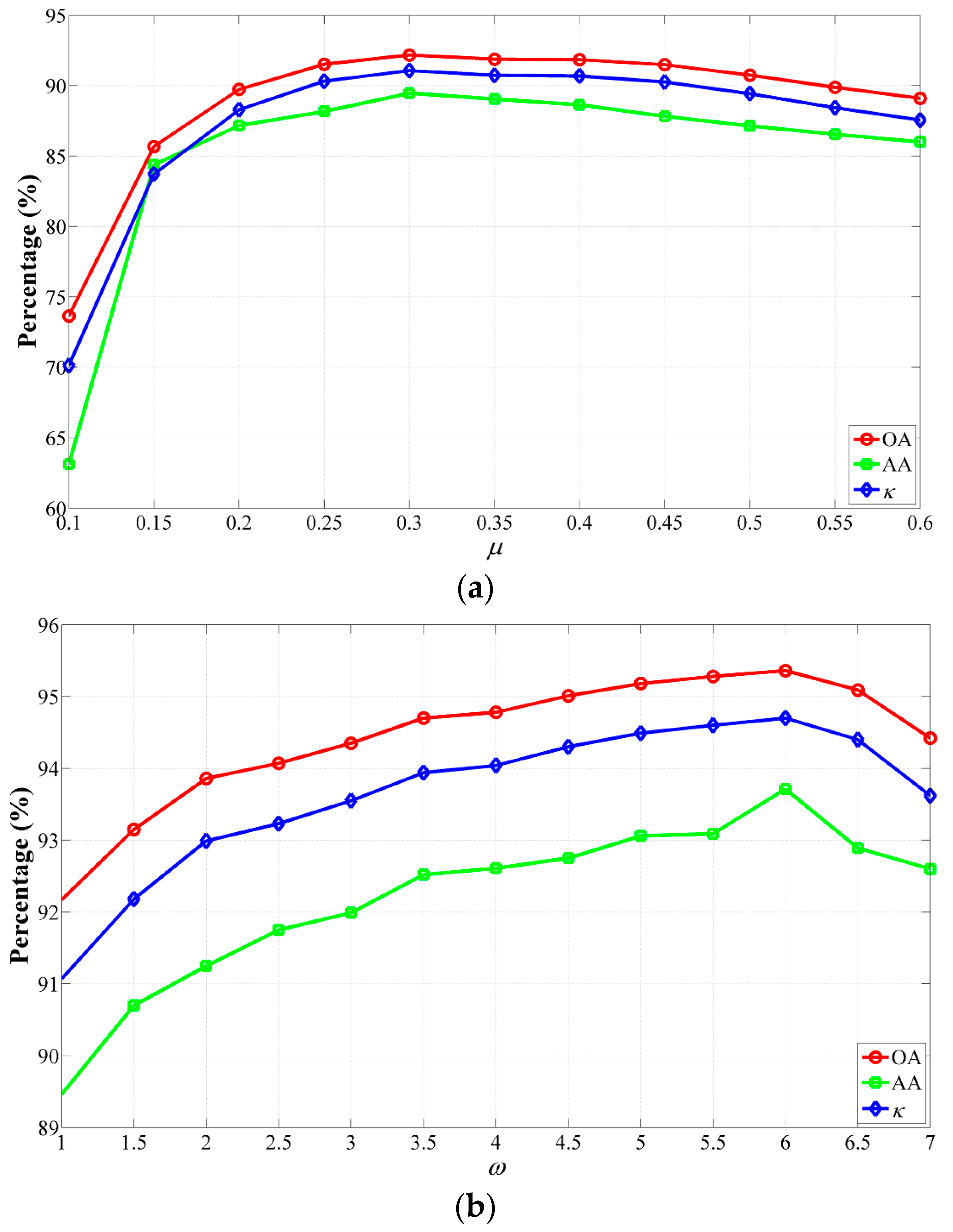
ω on classification accuracies using the CS-GC method for the Indian Pines data set is shown in Figure 8. Figure 8a demonstrates classification accuracies achieved by the CS-GC method varying μ from 0.1 to 0.6 with a step size of 0.05, while ω was set to be one. It can be observed from this figure that the shapes of these plots have a similar global behavior, i.e., the GAs rose rapidly as the increase of μ from 0.1 to 0.3 and decreased gradually as μ increased to 0.6. In addition, the highest GAs were obtained when μ = 0 . 3 with OA = 92 . 17 % , AA = 89 . 46 % and κ = 0 . 9107 . Meanwhile, Figure 8b illustrates the impact of ω varying from one to seven with a step size of 0.5 on the classification performance of the CS-GC method, while μ was set to be 0.3. Similarly, the GAs rose gradually as the increase of ω until the highest GAs were achieved when ω = 6 . Thus, in this case, the values of the OA, AA and κ increased from 92.17%, 89.46% and 0.9107 ( ω = 1 ) to 95.36%, 93.70% and 0.9470 ( ω = 6 ), respectively. However, these values declined to 94.42%, 92.60% and 0.9362 in the case of ω > 6 .
The impact of μ and 
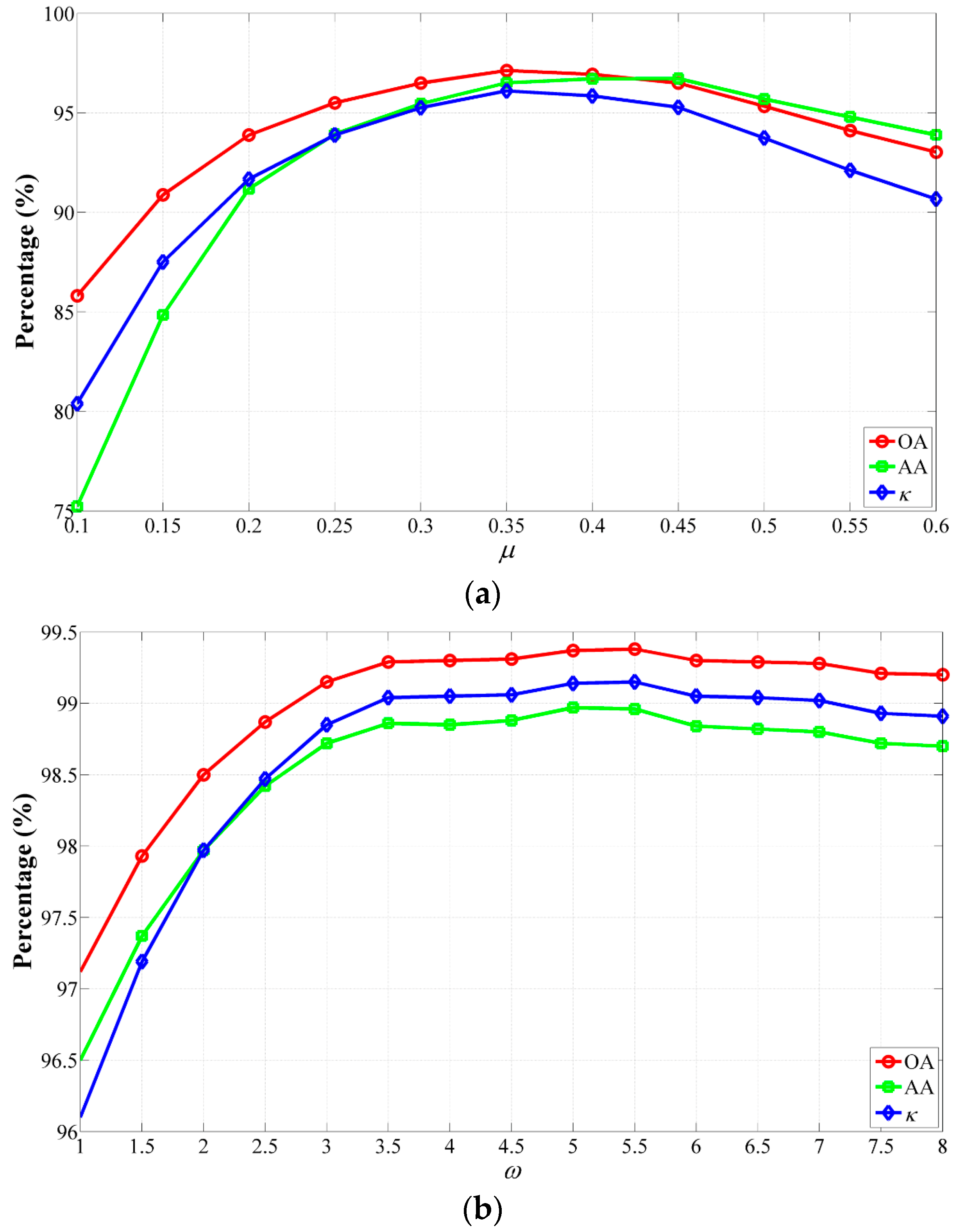
ω on classification accuracies using the CS-GC method for the University of Pavia data set is shown in Figure 9. (i) Figure 9a illustrates the GAs obtained using different values of μ from 0.1 to 0.6 with a step size of 0.05. In this case, ω was fixed at one. The plots of the GAs as the increase of μ were considerably similar to parabolas that open downward and the highest GAs were achieved in the case of μ = 0 . 35 with OA = 97 . 12 % , AA = 96 . 5 % and κ = 0 . 961 . Figure 9b depicts the GAs obtained using different values of ω from one to eight with a step size of 0.5 while μ was set to be 0.35. We can observe that the GAs were improved as the increase of μ. When ω increased to 5.5, the greatest GAs were obtained with OA = 99 . 38 % , AA = 98 . 96 % and κ = 0 . 9915 , which were 2.26%, 2.46% and 0.0305, respectively, higher than that using ω = 1 ; when ω increased from 5.5 to eight, the GAs continued to slide. Finally, the GAs of OA = 99 . 2 % , AA = 98 . 7 % and κ = 0 . 9891 
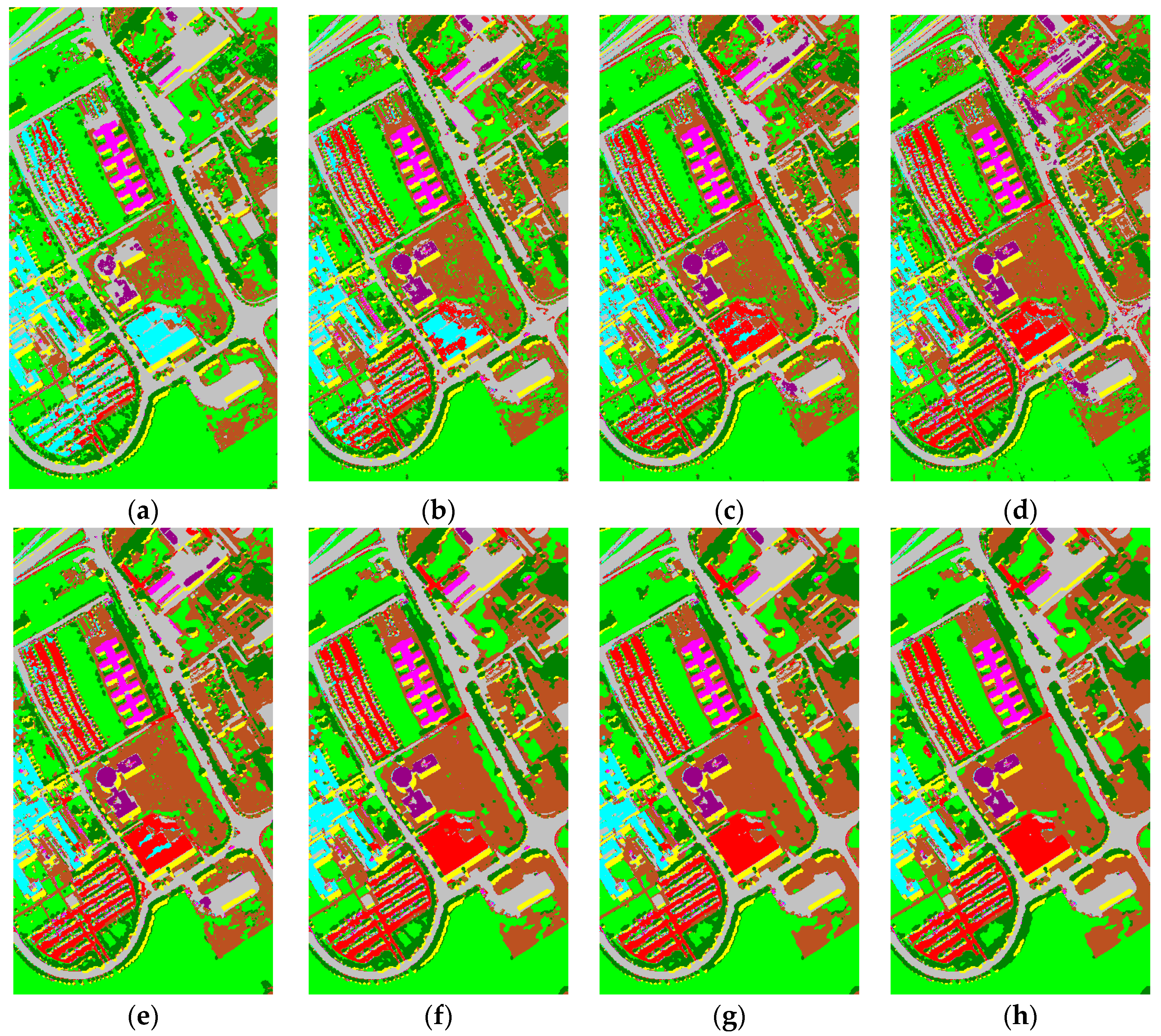
were obtained; (ii) To visually analyze the impacts of 
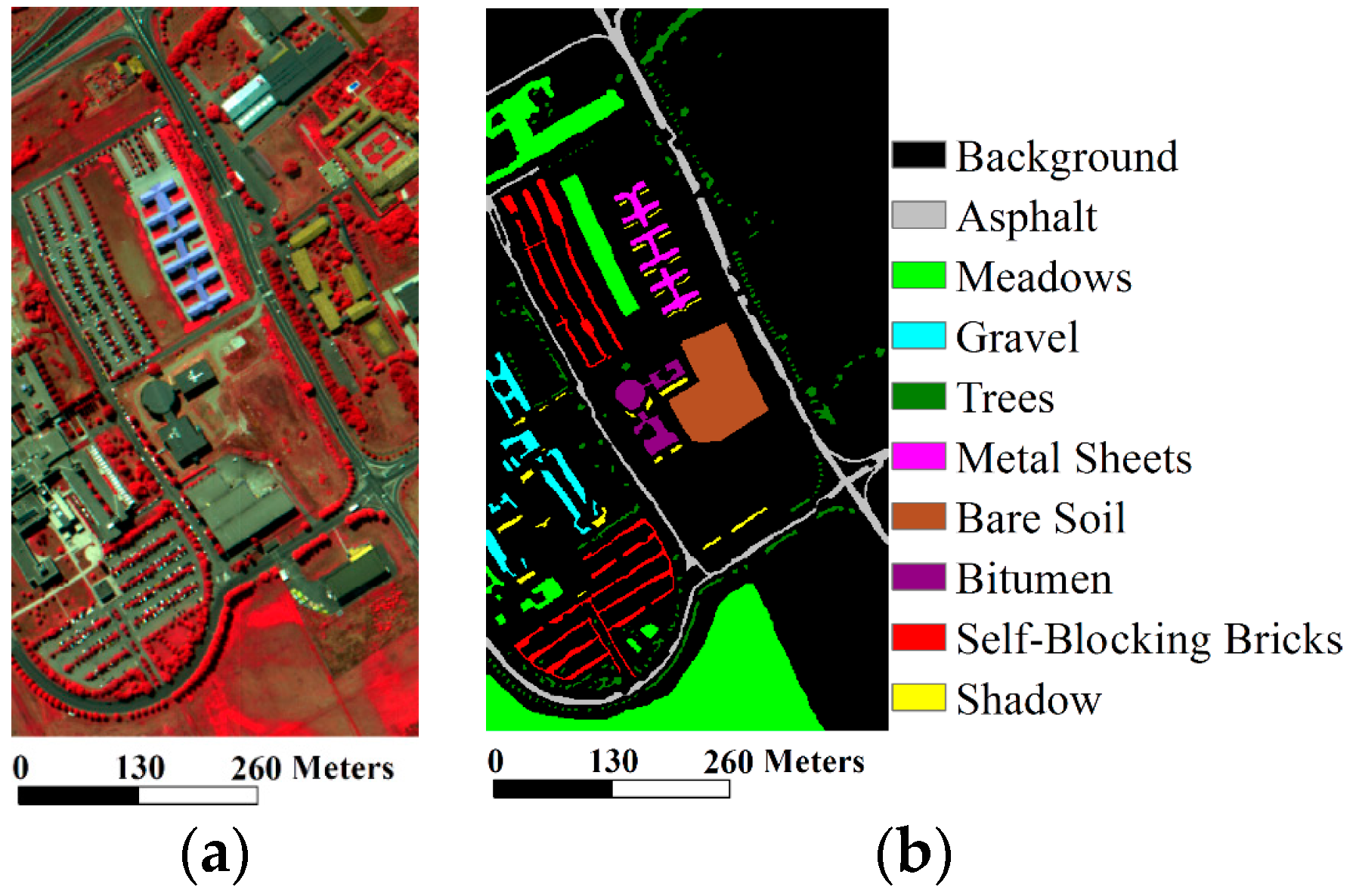
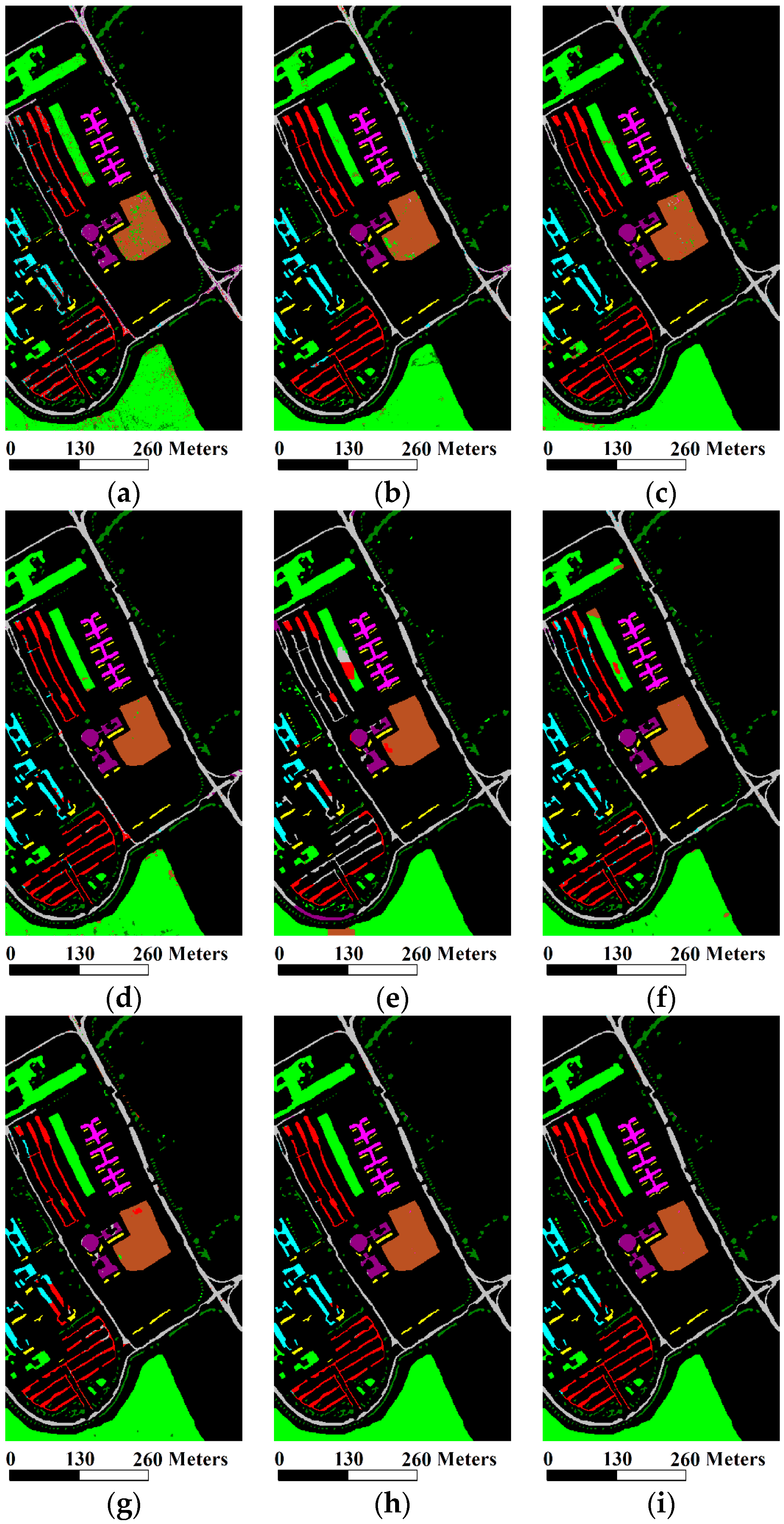
μ, the classification maps with different values of μ (0.15, 0.25, 0.35, 0.45) and ω = 1 are shown in Figure 10a–d, respectively. It can be found that the classes of Self-Blocking Bricks, Bitumen and Bare Soil cannot be effectively extracted if μ = 0 . 15 because smoothed probabilities of those classes were not very large. Meanwhile, some miscellaneous components appeared in the homogeneous regions of the classification maps if μ = 0 . 45 , especially in a region of Meadows at the bottom of the image. By comparison, we can obtain more accurate classification map when μ was fixed to be 0.35. To visually analyze the impacts of ω, the classification maps with different values of ω (2, 3, 4, and 5) are shown in Figure 10e–h, respectively. It is clear that salt-and-pepper noise in the classification maps can be well avoided as the increase of ω because more spatial information was integrated with spectral features of the hyperspectral data set in the CS-GC method. In addition, the classification map obtained by the CS-GC method using ω = 5 was better than the remaining resultant maps in terms of visual inspection. Specifically, regions in 
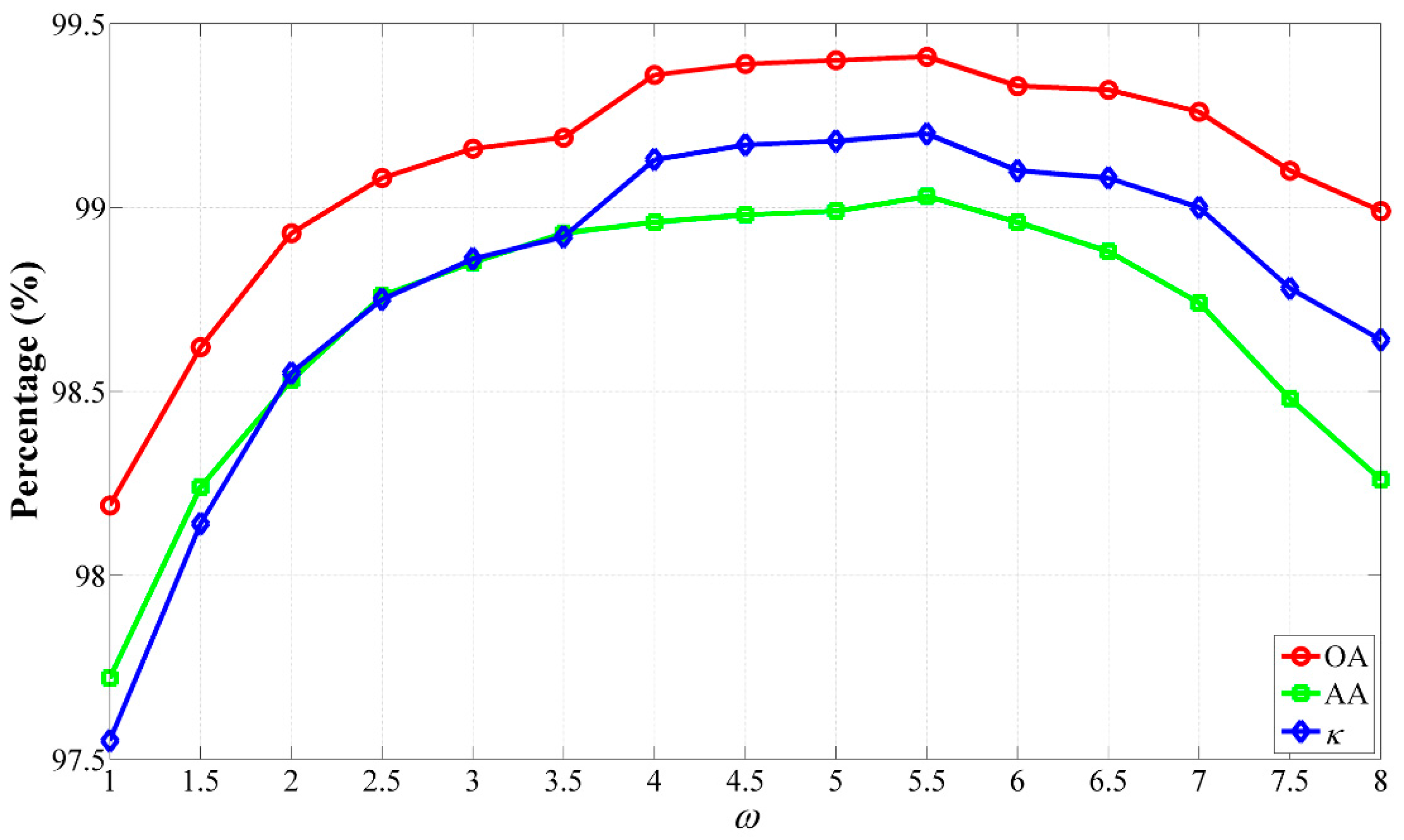
Figure 10h were well homogenized to completely remove class errors; (iii) To further analyze the impact of ω on classification accuracies, we applied the CS-GC + JBF method to the University of Pavia data set. In this experiment, ω was chosen from one to eight with a step size of 0.5 and the other parameters of the CS-GC + JBF method were set as μ = 0 . 35 , n = 1 , σ s = 8 and σ r = 0 . 01 . Figure 11 shows the GAs obtained using different values of ω. It can be found the GAs achieved by the CS-GC + JBF method were improved as the increase of ω from one to 5.5, and then reduced as the increase of ω from 5.5 to eight, which is consistent with the conclusion by using the CS-GC methods in terms of different values of ω. Meanwhile, it should be noted from this figure that the values of OA and κ are higher than 99% and 0.99, respectively, in the range of 4 ω 7 , which further validates the efficiency of the CS-GC + JBF method.
The impact of μ and 
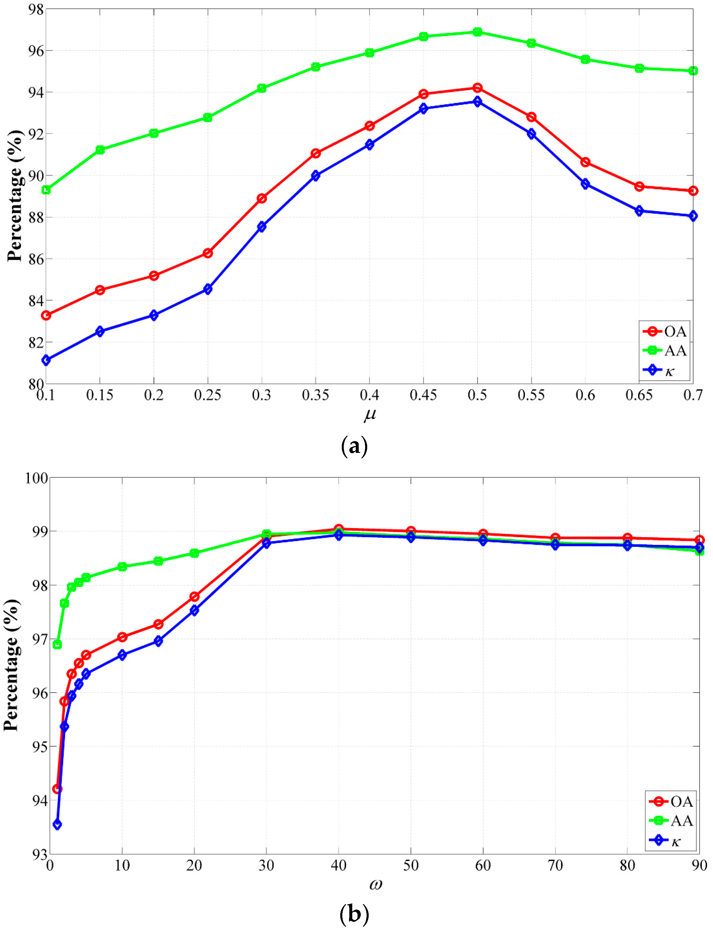
ω on classification accuracies using the CS-GC method for the Salinas data set is shown in Figure 12. The GAs plots obtained by using different values of μ from 0.1 to 0.7 with a step size of 0.05 and ω = 1 are shown in Figure 12a. From this figure, we can observe that the GAs kept increasing until μ increased to 0.5. However, when μ increased from 0.5 to 0.7, the GAs continued to slide. Therefore, the highest GAs were achieved in the case of μ = 0 . 5 with OA = 94 . 21 % , AA = 96 . 89 % and κ = 0 . 9355 . Meanwhile, the GAs plots obtained by using different values of ω from 0 to 90 with unequal steps and μ = 0 . 5 are demonstrated in Figure 12b. In this figure, the OA, AA and κ increased from 94.21%, 96.89% and 0.9355 ( ω = 1 ) to 99.04%, 98.97% and 0.9893 ( ω = 40 ), respectively, as the increase of ω from one to 40. In contrast, the GAs reduced very slowly in the range of 40 < ω 90 . Based on our experiments on the Salinas data set, including those not reported here, the GAs achieved by the CS-GC method were lower and can still maintain at high values even if ω was set very large. It should be noted that the range of ω for the Salinas data set was greatly different from that for the above two hyperspectral data sets, because the distribution of objects in the Salinas data set is more regular and all of regions in the ground truth data are quite large.
Based on the above experiments on the impact analysis of μ and ω, we can draw conclusions as follows:
(1) Since the strength of spectral weights in the procedure of image classification is modulated by μ, we can consider this parameter as a spectral weight regulator. As mentioned in Section 3, the proposed method performs segmentation based on the competition between object (each class) and background in the energy functional Equation (13). If the value of μ is close to one, the “background” is dominant in the competition. Otherwise, if the value of μ is close to 0, the energy functional is apt to superiorly separate targets of a certain class from backgrounds. Therefore, the appropriate setting of the spectral weight regulator plays an important role for exacting information classes from hyperspectral images. Experiments on the three hyperspectral datasets demonstrated that the plots of the GAs as the increase of μ were approximately a concave shape and the highest GAs can be achieved using an appropriate setting of μ.
(2) The parameter ω is used to balance the data and smoothness terms. In this work, it is also employed as a spatial weight regulator. For instance, the increase of ω contributes to accurately extracting spatial information and improving classification accuracies due to similarities between the central pixel and its neighborhoods. However, if the value of ω is set too large, the smoothness term plays a major role in the energy functional. Therefore, some information class regions always contain small-scale regions belonging to other classes, which leads to the reduction of classification accuracies.
(3) We can observe that our method can achieve the highest classification accuracies on the Indian Pines data set with a relatively small value of μ, by comparing Figure 8a with Figure 9a and Figure 12a, due to the fact that the ground objects in the Indian Pines data set are mainly the corps and this image includes more small-scale homogeneous regions that are spatially and spectrally similar. Although the other two data sets are composed of different types of ground objects, the distribution of all the different objects in the Salinas data set is much more regular and the corresponding homogeneous regions are quite large, compared to the University of Pavia data set. As a consequence, a relative large value of μ is required for our method to achieve the best classification accuracies on the Salinas data set. Therefore, for classification of unlabeled data, μ should be a data-dependent parameter. (i) If the unlabeled data include many small-scale homogeneous regions that are spatially and spectrally close like the Indian Pines data set, a small value of μ is recommended. For instance, the default value of μ can be set as μ = 0.3; (ii) If the unlabeled data contain different types of ground objects and shapes of these objects are very regular, μ can be set as a large value, e.g., μ = 0.5; (iii) If there is no prior knowledge, considering the classification performance, we recommend selecting a relatively moderate value of μ as μ = 0.4. Similarly, ω should be a data-dependent parameter as well. (i) If the unlabeled data are spatially and spectrally close like the University of Pavia image, i.e., the unlabeled data contain different types of ground objects and the distribution of those objects in the unlabeled data is unbalanced, a small value of ω is recommended, e.g., ω = 3; (ii) If the unlabeled data mainly include the ground objects with quite regular boundaries and the distribution of all the ground objects is relatively uniform like the Salinas image, ω can be set as a relatively small value to obtain satisfactory results, e.g., ω = 30; (iii) If there is no prior knowledge, considering the classification performance, we recommend selecting a relatively moderate value of ω as 5 ω 10 .
(2) Influence of n, σs and σr
Then, we perform the proposed CS-GC + JBF method to analyze the impact of the parameters in the JBF. As mentioned in Section 3.2, our JBF can greatly avoid unstable distribution of class membership probabilities caused by a pixel-wise classifier only taking spectral features in the image into account. Not only does the proposed JBF well preserve important edges in the image, but also spatially optimize class membership probabilities. Therefore, we may not achieve the highest GAs using the optimal parameter setting of μ and ω obtained from Figure 9, especially for the spatial weight regulator ω. Based on our experiments on the Indian Pines data set, including those not reported here, these two parameters for the CS-GC + JBF method were set as μ = 0 . 3 and ω = 2 .
The impact of n, σs and σr on classification accuracies using the proposed CS-GC + JBF method for the Indian Pines data set is shown in Table 5. (i) To analyze the impact of the size of local window on classification accuracies, we applied the CS-GC + JBF method to classify the Indian Pines image by setting different values of n from one to five and the corresponding window sizes and GAs are listed in Table 5. In our method, the other parameters were set as σ s = 4 and σ r = 0 . 01 . It should be noted that the GAs in Table 5 at the value of “0” in terms of different parameters mean that they were achieved by our CS-GC method (without the optional JBF step) for the Indian Pines image. In addition, it can be seen from this table that the highest OA and κ can be reached when the size of local window was 7 × 7, i.e., n = 3 . If n is too large, small-scale regions belonging to a certain class are always smoothed out by the JBF, which may cause the decrease of classification accuracies; while if n is too small, our method cannot considerably smooth out salt-and-pepper classification noise caused by the pixel-wise classification and avoid unstable distribution of class membership probabilities; (ii) To analyze the impact of σ s on classification accuracies, we applied the CS-GC + JBF method to classify the Indian Pines image by selecting different values (0.5, 1, 2, 4, and 8) and the corresponding GAs are listed in Table 5 as well. In our method, the other parameters were set as n = 3 and σ r = 0 . 01 . A similar conclusion can be drawn that σ s should not be set to be too large or small and the highest OA and κ were achieved in the case of σ s = 4 
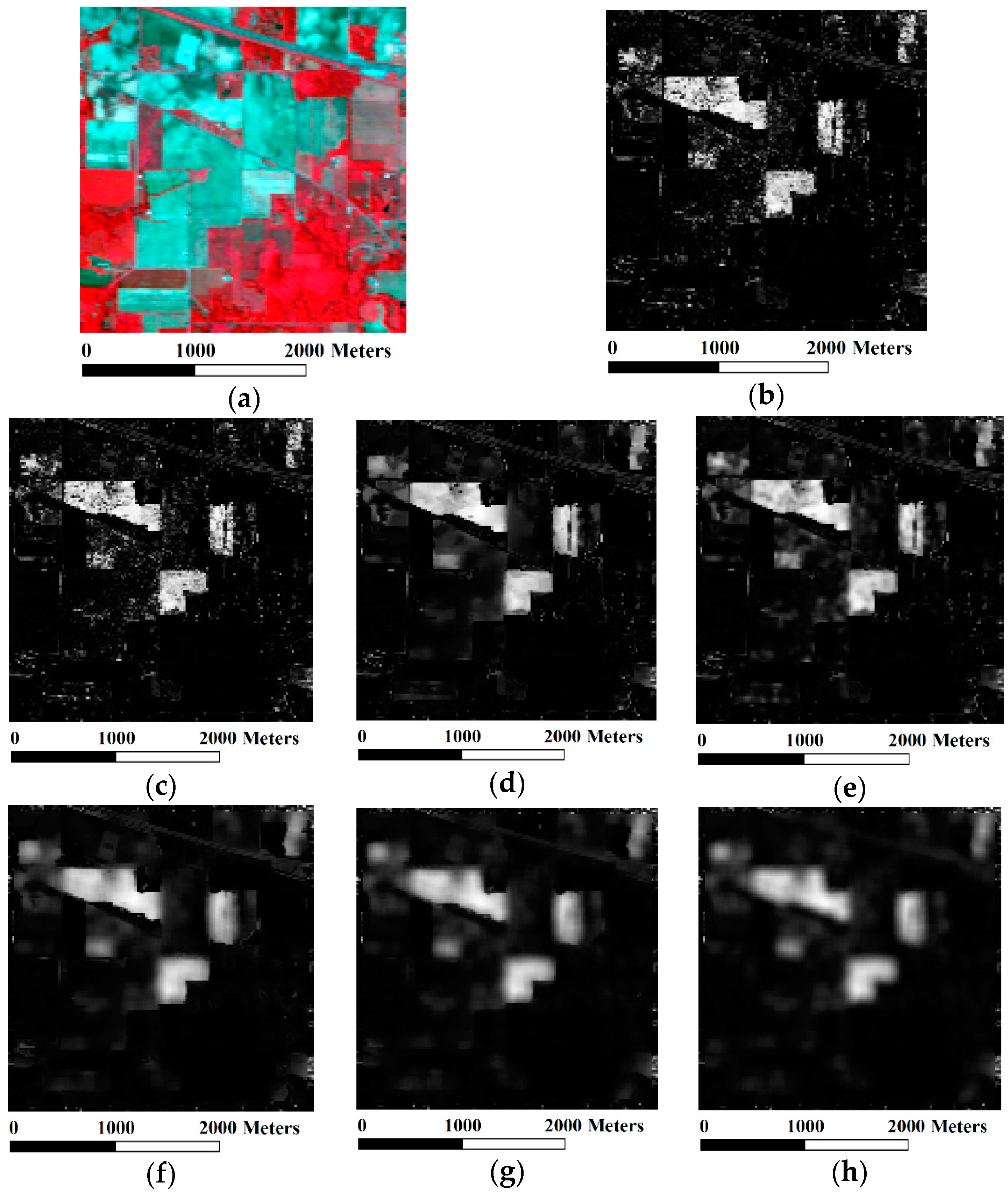
; (iii) It can be observed from Equation (8) that the setting of σr is vitally important to the performance of our JFB. To analyze the impact of σr on classification accuracies, we provided an example of probability smoothing by selecting different values of σr (0.001, 0.005, 0.01, 0.02, 0.04, and 0.1). The corresponding smoothed probability maps in terms of Corn-no till are shown in Figure 13. The other parameters for the JBF were set as n = 3 and σ s = 4 . We can observe from this figure that the smoothing effect was very limited when σr was equal to 0.001. As σr increased, the salt-and-pepper classification noise in the probability map was gradually removed while edges were well preserved. However, the proposed JBF leaded to oversmoothing on the probability map and edges of Corn-no till were seriously blurred in the case of σ r = 0 . 1 . To better analyze the impact of σr on classification accuracies, this parameter was set from 0.005 to 0.03 with a step size of 0.005 and the other parameters were the same as that used in Figure 9. It can be easily observed from Table 5 that the GAs shared the same tendency as the above experiments when analyzing the impacts of n and σs. For instance, the OA and κ increased in the case of σ r < 0 . 015 and the highest OA and κ can be achieved when σr was equal to 0.015. However, these two measures decreased in the case of σ r > 0 . 015 . Meanwhile, the extremum value of σr was 0.02 in terms of the AA.
Then, we performed the CS-GC + JBF method on the University of Pavia data set to analyze the impact of n, σ s and σ r on classification accuracies. To analyze the impact of n, we provided a set of n (1, 2, 3, 4, and 5) and the other parameters were fixed as μ = 0 . 35 , ω = 2 , σ s = 4 and σ r = 0 . 01 ; to analyze the impact of σ s on classification accuracies, we gave a set of σ s (0, 0.5, 1, 2, 4, and 8) and the other parameters were fixed as μ = 0 . 35 , ω = 2 , n = 2 and σ r = 0 . 01 ; and to analyze the impact of σ r on classification accuracies, we presented a set of σ r from 0 to 0.03 with a step size of 0.005 and the other parameters were fixed as μ = 0 . 35 , ω = 5 . 5 , n = 1 and σ s = 4 . The corresponding GAs in terms of different parameter settings are reported in Table 6. It can be seen that the trend of the GAs, as the increase of n, σ s or σ r , was similar to that in the first experiment for the Indian Pines data set.
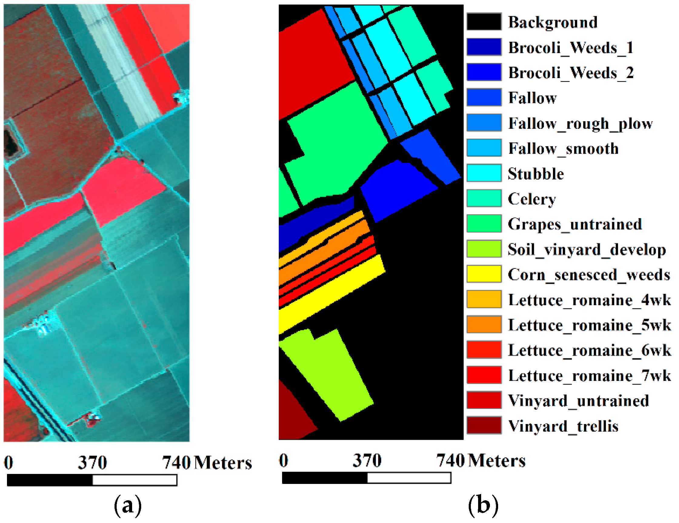
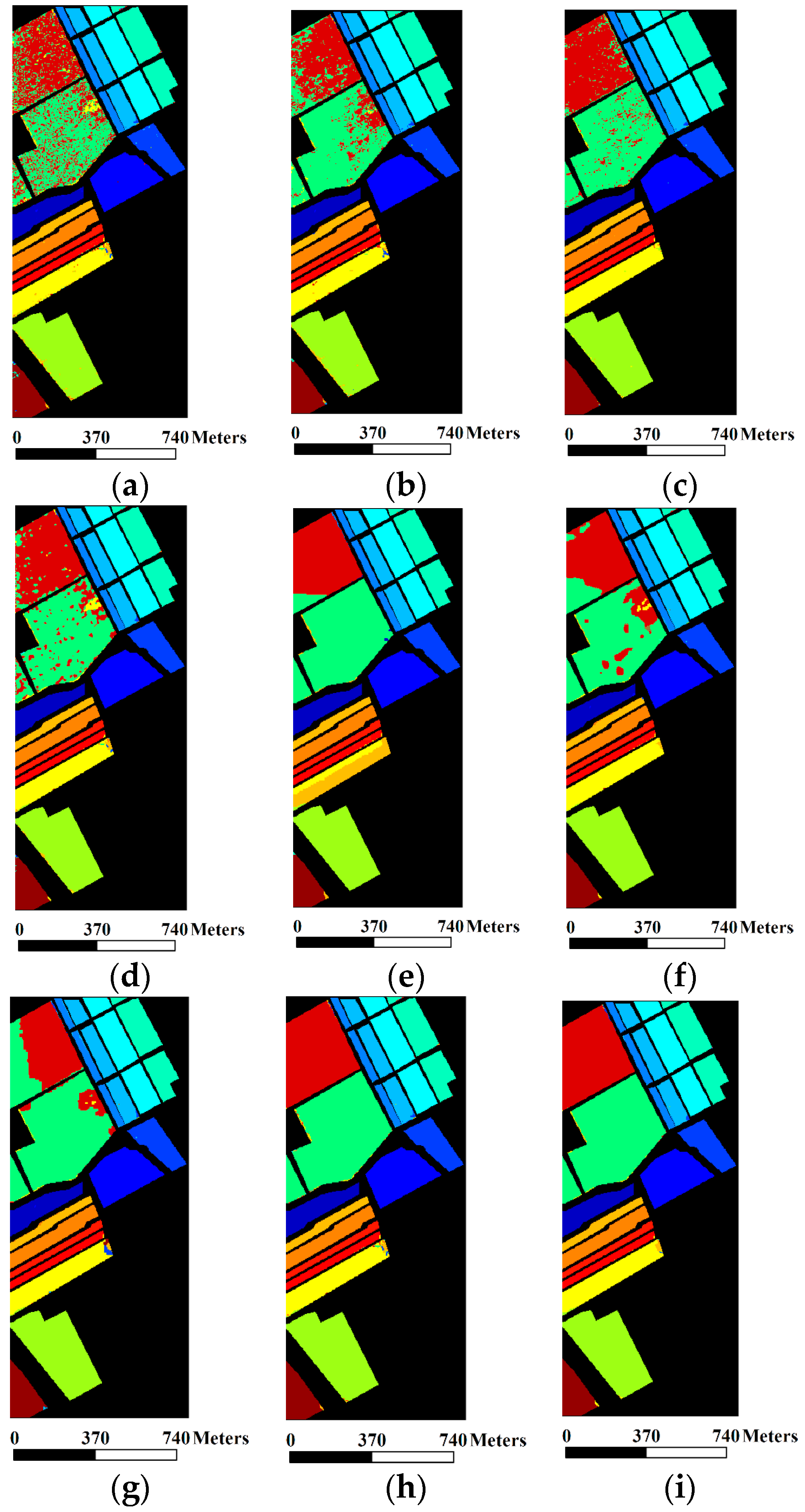
Finally, we performed the CS-GC + JBF method on the Salinas data set to analyze the impact of n, σ s and σ r on classification accuracies with μ = 0 . 5 , ω = 5 and the corresponding GAs in terms of different parameter settings are reported in Table 7. To analyze the impact of n, n was set from one to five with a step size of one and the other parameters were fixed as σ s = 4 and σ r = 0 . 01 . In Table 7, the GAs were improved as the increase of n due to the fact that a very large local window is required for smoothing out the noise in large-scale regions in the image. To analyze the impact of σ s , σ s was chosen from (0, 0.5, 1, 2, 4, and 8) and the other parameters were fixed as n = 2 and σ r = 0 . 01 ; to analyze the impact of σ r , σ r was set from 0.01 to 0.035 with a step size of 0.005 and the other parameters were fixed as n = 2 and σ s = 4 . It can be observed that the trend of the GAs, as the increase of σ s or σ r , is completely consistent with the previous experiments. In addition, the highest GAs can be obtained using the CS-GC + JBF method with σ s = 4 when varying σ s from 0 to eight; the highest GAs can be obtained using the CS-GC + JBF method with σ r = 0 . 025 when varying σ r from 0.01 to 0.035, as shown in 
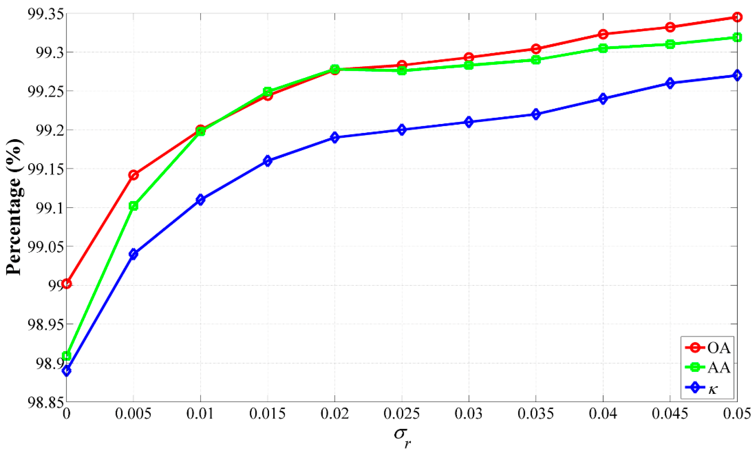
Table 7. To further analyze the impact of σ r on classification accuracies, we applied the CS-GC + JBF method to the Salinas data set. In this experiment, σ r was chosen from 0 to 0.05 with a step size of 0.005 and the other parameters of the CS-GC + JBF method were set as μ = 0 . 5 , ω = 50 , n = 2 and σ s = 4 . The GAs plots obtained by the CS-GC + JBF method using different values of σ r ( 0 σ r 0 . 05 ) are demonstrated in Figure 14. We observed that the GAs achieved by the CS-GC + JBF method increased fast as the rising of σ r from 0 to 0.02, while if σ r was larger than 0.02, the increase of the GAs slowed down. Finally, the highest OA, AA and κ achieved by the CS-GC + JBF method with σ r = 0 . 05 can reach 99.35%, 99.32% and 0.9927, respectively. It is noteworthy that the main difference between the impacts of σ r in Figure 14 and Table 7 on classification accuracies stems from the different ranges of ω.
It can be seen in Table 5, Table 6 and Table 7 that the CS-GC + JBF method is not very sensitive to σ s and σ s = 4 performs the best for our method on all of the three data sets. In addition, it should be noted that the University of Pavia data set is composed of different types of ground objects. Furthermore, those objects on the image are unevenly distributed. As a consequence, edge strengths of the object boundaries vary in a wide range. To better preserve most important edge features of this data set for the subsequent classification, a relatively small value of σ r is preferred. As mentioned above, the ground objects are mainly the corps in the Indian Pines data set, thus edge strengths of the object boundaries change very little, a slightly large value of σ r can ensure that noise in the probability maps is thoroughly removed while edges are effectively preserved. Since the Salinas data set is composed by mainly different types of vegetation and the object boundaries are very regular for observation, a relatively large value of σ r is required for our method to achieve the best classification performance.
In conclusion, for classification of unlabeled data, σ s can be the same as σ s = 4 for our method to achieve the best classification accuracies, while σ r should be a data-dependent parameter. (i) If the unlabeled data contain different types of ground objects and edge strengths of the object boundaries are very different, a small value of σ r is recommended. For instance, the default value of σ r can be set as σ r = 0 . 01 ; (ii) If boundaries of ground objects in the unlabeled data are obvious and their shapes are very regular, σ r can be set as a large value, σ r = 0 . 025 ; (iii) If there is no prior knowledge, considering the classification performance, we recommend selecting a relatively moderate value of σ r as σ r = 0 . 015 .

5.2. Classification Results with Different Number of Training Samples

In this subsection, the influence of different training samples to the stability of the CS-GC + JBF method is analyzed. Experiments were performed on two datasets, i.e., the Indian Pines data set and the University of Pavia data set. To better demonstrate the performance of our method, the SVM method was used for comparison and the default parameter settings of these methods were fixed the same as the previous experiments in Section 4. The number of training samples for each class used by the two methods increased from 5% to 50% for the Indian Pines data set with a step size of 5%, and 1% to 10% for the University of Pavia data set with a step size of 1%. To accurately obtain the classification results, the OA values obtained by the two methods with different training samples were the average results over five trials. Figure 15 illustrates the evolution of the OA obtained by the two comparative methods with different number of training samples for the two hyperspectral datasets. It can be observed from this figure that the OA values achieved by the two classification methods were positively correlated with the number of training samples. Meanwhile, our method was superior to the SVM method with the same number of training samples for the two hyperspectral datasets. For instance, regarding the Indian Pines image, when the OA achieved by the SAM method is 82.51% with 10% ground truth samples are used for training, the CS-GC + JBF method can reach over 96%. A similar conclusion can be drawn based on the experimental results in terms of the University of Pavia data set.

6. Conclusions

In this paper, a novel framework to perform spatial-spectral classification of hyperspectral images is presented. The major contribution of this work is to explore an alternative technique for labeling regions obtained by the segmentation process using JBF and graph cut based model. In our algorithm, the optional step of JBF can remove salt-and-pepper class noise and effectively preserve important boundaries of ground objects in the image, while the CS-GC model can successfully extract each of the desirable objects using the minimum cut algorithm. The proposed methods were compared with several classical hyperspectral image classification methods using objective quantitative measures and a visual qualitative evaluation. Experimental results demonstrated that our methods were better than the other methods in terms of the GAs, while the CS-GC + JBF method can obtain improvements of 13.68%, 8.56% and 10.2% in terms of OA over the pixel-wise SVM classifier for the Indian Pines, University of Pavia and Salinas datasets, respectively. Furthermore, for all three datasets, the GAs by the CS-GC + JBF method were the best among all of the classification methods for hyperspectral images. It can be concluded from the experimental results that the integration of the extended JBF with our CS-GC model can obtain more accurate classification results of hyperspectral images. Furthermore, the proposed CS-GC + JBF method was robust relative to the three parameters and we recommend μ = 0.4, 5 ω 10 , σ s = 4 and σ r = 0 . 015 .
In the future, adaptive modulation techniques of the parameters for our methods are required for improving their efficiency and universality. For instance, a further improvement may be achieved by adaptively modulating the spectral weight regulator μ with respect to different information classes. Finally, the efficient parallel implementation of our methods is possible.

Acknowledgments

This work was supported by the National Natural Science Foundation of China (61271408).

Author Contributions

Yi Wang, Haiwei Song and Yan Zhang implemented the proposed classification method and conducted the experiments. Haiwei Song finished the first draft. Yi Wang supervised the research and contributed to the editing and review of the manuscript.

Conflicts of Interest

The authors declare no conflict of interest.

References

  1. Plaza, A.; Benediktsson, J.A.; Boardman, J.W.; Brazile, J.; Bruzzone, L.; Camps-Valls, G.; Chanussot, J.; Fauvel, M.; Gamba, P.; Gualtieri, A.; et al. Recent advances in techniques for hyperspectral image processing. Remote Sens. Environ. 2009, 113, S110–S122. [Google Scholar] [CrossRef]
  2. Camps-Valls, G.; Tuia, D.; Bruzzone, L.; Benediktsson, J.A. Advances in hyperspectral image classification: Earth monitoring with statistical learning methods. IEEE Signal Peocess. Mag. 2014, 31, 45–54. [Google Scholar] [CrossRef]
  3. Melgani, F.; Bruzzone, L. Classification of hyperspectral remote sensing images with support vector machines. IEEE Trans. Geosci. Remote Sens. 2004, 42, 1778–1790. [Google Scholar] [CrossRef]
  4. Camps-Valls, G.; Bruzzone, L. Kernel-based methods for hyperspectral image classification. IEEE Trans. Geosci. Remote Sens. 2005, 43, 1351–1362. [Google Scholar] [CrossRef]
  5. Zhang, Y. Optimisation of building detection in satellite images by combining multispectral classification and texture filtering. ISPRS J. Photogramm. Remote Sens. 1999, 54, 50–60. [Google Scholar] [CrossRef]
  6. Huang, X.; Zhang, L. A comparative study of spatial approaches for urban mapping using hyperspectral rosis images over pavia city, northern italy. Int. J. Remote Sens. 2009, 30, 3205–3221. [Google Scholar] [CrossRef]
  7. Benediktsson, J.A.; Palmason, J.A.; Sveinsson, J.R. Classification of hyperspectral data from urban areas based on extended morphological profiles. IEEE Trans. Geosci. Remote Sens. 2005, 43, 480–491. [Google Scholar] [CrossRef]
  8. Zhang, L.; Huang, X.; Huang, B.; Li, P. A pixel shape index coupled with spectral information for classification of high spatial resolution remotely sensed imagery. IEEE Trans. Geosci. Remote Sens. 2006, 44, 2950–2961. [Google Scholar] [CrossRef]
  9. Mura, M.D.; Villa, A.; Benediktsson, J.A.; Chanussot, J.; Bruzzone, L. Classification of hyperspectral images by using extended morphological attribute profiles and independent component analysis. IEEE Geosci. Remote Sens. Lett. 2011, 8, 542–546. [Google Scholar] [CrossRef]
  10. Shen, L.; Zhu, Z.; Jia, S.; Zhu, J.; Sun, Y. Discriminative gabor feature selection for hyperspectral image classification. IEEE Geosci. Remote Sens. Lett. 2013, 10, 29–33. [Google Scholar] [CrossRef]
  11. Chen, C.; Li, W.; Su, H.; Liu, K. Spectral-spatial classification of hyperspectral image based on kernel extreme learning machine. Remote Sens. 2014, 6, 5795–5814. [Google Scholar] [CrossRef]
  12. Qian, Y.; Ye, M.; Zhou, J. Hyperspectral image classification based on structured sparse logistic regression and three-dimensional wavelet texture features. IEEE Trans. Geosci. Remote Sens. 2013, 51, 2276–2291. [Google Scholar] [CrossRef]
  13. Quesada-Barriuso, P.; Argüello, F.; Heras, D.B. Spectral-spatial classification of hyperspectral images using wavelets and extended morphological profiles. IEEE J. Sel. Top. Appl. Earth Obs. Remote Sens. 2014, 7, 1177–1185. [Google Scholar] [CrossRef]
  14. Quesada-Barriuso, P.; Argüello, F.; Heras, D.B.; Benediktsson, J.A. Wavelet-based classification of hyperspectral images using extended morphological profiles on graphics processing units. IEEE J. Sel. Top. Appl. Earth Obs. Remote Sens. 2015, 8, 2962–2970. [Google Scholar] [CrossRef]
  15. Tarabalka, Y.; Chanussot, J.; Benediktsson, J.A. Segmentation and classification of hyperspectral images using watershed transformation. Pattern Recognit. 2010, 43, 2367–2379. [Google Scholar] [CrossRef]
  16. Huang, X.; Zhang, L. An adaptive mean-shift analysis approach for object extraction and classification from urban hyperspectral imagery. IEEE Trans. Geosci. Remote Sens. 2008, 46, 4173–4185. [Google Scholar] [CrossRef]
  17. Ghamisi, P.; Couceiro, M.S.; Fauvel, M.; Benediktsson, J.A. Integration of segmentation techniques for classification of hyperspectral images. IEEE Geosci. Remote Sens. Lett. 2014, 11, 342–346. [Google Scholar] [CrossRef]
  18. Tarabalka, Y.; Tilton, J.C.; Benediktsson, J.A.; Chanussot, J. A marker-based approach for the automated selection of a single segmentation from a hierarchical set of image segmentations. IEEE J. Sel. Top. Appl. Earth Obs. Remote Sens. 2012, 5, 262–272. [Google Scholar] [CrossRef]
  19. Song, H.; Wang, Y. A spectral-spatial hyperspectral image classification based on algebraic multigrid methods and hierarchical segmentation. Remote Sens. 2016, 8, 296. [Google Scholar] [CrossRef]
  20. Fang, L.; Li, S.; Kang, X.; Benediktsson, J.A. Spectral-spatial classification of hyperspectral images with a superpixel-based discriminative sparse model. IEEE Trans. Geosci. Remote Sens. 2015, 53, 4186–4201. [Google Scholar] [CrossRef]
  21. Kettig, R.L.; Landgrebe, D.A. Classification of multispectral image data by extraction and classification of homogeneous objects. IEEE Trans. Geosci. Electron. 1976, 14, 19–26. [Google Scholar] [CrossRef]
  22. Tarabalka, Y.; Chanussot, J.; Benediktsson, J.A. Segmentation and classification of hyperspectral images using minimum spanning forest grown from automatically selected markers. IEEE Trans. Syst. Man Cybern. Part B Cybern. 2010, 40, 1267–1279. [Google Scholar] [CrossRef] [PubMed]
  23. Tuia, D.; Camps-Valls, G.; Matasci, G.; Kanevski, M. Learning relevant image features with multiple kernel classification. IEEE Trans. Geosci. Remote Sens. 2010, 48, 3780–3791. [Google Scholar] [CrossRef]
  24. Li, J.; Marpu, P.R.; Plaza, A.; Bioucas-Dias, J.M.; Benediktsson, J.A. Generalized composite kernel framework for hyperspectral image classification. IEEE Trans. Geosci. Remote Sens. 2013, 51, 4816–4829. [Google Scholar] [CrossRef]
  25. Mathieu, F.; Jocelyn, C.; Atli, B.J. A spatial–spectral kernel-based approach for the classification of remote-sensing images. Pattern Recognit. 2012, 45, 381–392. [Google Scholar]
  26. Kolmogorov, V.; Zabin, R. What energy functions can be minimized via graph cuts? IEEE Trans. Pattern Anal. Mach. Intell. 2004, 26, 147–159. [Google Scholar] [CrossRef] [PubMed]
  27. Amini, A.A.; Weymouth, T.E.; Jain, R.C. Using dynamic programming for solving variational problems in vision. IEEE Trans. Pattern Anal. Mach. Intell. 1990, 12, 855–867. [Google Scholar] [CrossRef]
  28. Peng, B.; Zhang, L.; Zhang, D. A survey of graph theoretical approaches to image segmentation. Pattern Recognit. 2013, 46, 1020–1038. [Google Scholar] [CrossRef]
  29. Yu, X.; Niu, R.; Wang, Y.; Wu, K. Multiscale graph cut based classification of urban hyperspectral imagery. In Multispectral Image Processing and Pattern Recognition; SPIE: Bellingham, WA, USA, 2009; pp. 1–9. [Google Scholar]
  30. Tarabalka, Y.; Rana, A. Graph-cut-based model for spectral-spatial classification of hyperspectral images. In Proceedings of the IEEE Geoscience and Remote Sensing Symposium, Quebec, QC, Canada, 13–18 July 2014.
  31. Ma, L.; Ma, A.; Ju, C.; Li, X. Graph-based semi-supervise d learning for spectral-spatial hyperspectral image classification. Pattern Recognit. Lett. 2016. [Google Scholar] [CrossRef]
  32. Bai, J.; Xiang, S.; Pan, C. A graph-based classification method for hyperspectral images. IEEE Trans. Geosci. Remote Sens. 2013, 51, 803–817. [Google Scholar] [CrossRef]
  33. Jia, S.; Zhang, X.; Li, Q. Spectral-spatial hyperspectral image classification using l1/2 regularized low-rank representation and sparse representation-based graph cuts. IEEE J. Sel. Top. Appl. Earth Obs. Remote Sens. 2015, 8, 2473–2484. [Google Scholar] [CrossRef]
  34. Damodaran, B.B.; Nidamanuri, R.R.; Tarabalka, Y. Dynamic ensemble selection approach for hyperspectral image classification with joint spectral and spatial information. IEEE J. Sel. Top. Appl. Earth Obs. Remote Sens. 2015, 8, 2405–2417. [Google Scholar] [CrossRef]
  35. Tomasi, C.; Manduchi, R. Bilateral filtering for gray and color images. In Proceedings of the Sixth International Conference on Computer Vision, Bombay, India, 4–7 January 1998.
  36. Shi, J.; Fowlkes, C.; Martin, D.; Sharon, E. Graph Based Image Segmentation Tutorial. Available online: http://www.cis.upenn.edu/~jshi/GraphTutorial/ (accessed on 27 June 2004).
  37. Ford, D.R.; Fulkerson, D.R. Flows in Networks; Princeton University Press: Princeton, NJ, USA, 2010. [Google Scholar]
  38. Boykov, Y.; Kolmogorov, V. An experimental comparison of min-cut/max-flow algorithms for energy minimization in vision. IEEE Trans. Pattern Anal. Mach. Intell. 2004, 26, 1124–1137. [Google Scholar] [CrossRef] [PubMed]
  39. Boykov, Y.Y.; Jolly, M.-P. Interactive graph cuts for optimal boundary & region segmentation of objects in ND images. In Proceedings of the Internation Conference on Computer Vision, Vancouver, BC, Canada, 13 July 2001.
  40. Boykov, Y.; Funka-Lea, G. Graph cuts and efficient n-d image segmentation. Int. J. Comput. Vis. 2006, 70, 109–131. [Google Scholar] [CrossRef]
  41. Chang, C.-C.; Lin, C.-J. Libsvm: A library for support vector machines. ACM Trans. Intell. Syst. Technol. 2011. [Google Scholar] [CrossRef]
  42. Wu, T.-F.; Lin, C.J.; Weng, R.C. Probability estimates for multiclass classification by pairwise coupling. J. Mach. Learn. Res. 2004, 5, 975–1005. [Google Scholar]
  43. Vapnik, V.N. Statistical Learning Theory; Wiley: New York, NY, USA, 1998. [Google Scholar]
  44. Paris, S.; Kornprobst, P.; Tumblin, J.; Durand, F. Bilateral filtering: Theory and applications. Found. Trends Comput. Graph. Vis. 2009, 4, 1–73. [Google Scholar] [CrossRef]
  45. Petschnigg, G.; Szeliski, R.; Agrawala, M.; Cohen, M.; Hoppe, H.; Toyama, K. Digital photography with flash and no-flash image pairs. ACM Trans. Graph. 2004, 23, 664–672. [Google Scholar] [CrossRef]
  46. Rother, C.; Kolmogorov, V.; Blake, A. Grabcut: Interactive foreground extraction using iterated graph cuts. ACM Trans. Graph. 2004, 23, 309–314. [Google Scholar] [CrossRef]
  47. Kang, X.; Li, S.; Benediktsson, J.A. Spectral-spatial hyperspectral image classification with edge-preserving filtering. IEEE Trans. Geosci. Remote Sens. 2014, 52, 2666–2677. [Google Scholar] [CrossRef]
  48. Li, J.; Bioucas-Dias, J.M.; Plaza, A. Spectral-spatial classification of hyperspectral data using loopy belief propagation and active learning. IEEE Trans. Geosci. Remote Sens. 2013, 51, 844–856. [Google Scholar] [CrossRef]
  49. Bioucas-Dias, J.M.; Figueiredo, M. Logistic Regression via Variable Splitting and Augmented Lagrangian Tools; Instituto Superior Tecnico: Lisboa, Portugal, 2009. [Google Scholar]
  50. Li, J.; Bioucas-Dias, J.M.; Plaza, A. Hyperspectral image segmentation using a new bayesian approach with active learning. IEEE Trans. Geosci. Remote Sens. 2011, 49, 3947–3960. [Google Scholar] [CrossRef]
  51. Li, J. The Source Codes of the MLR-LORSAL, LBP-AL and LORSAR-AL-MLL Methods. Available online: http://www.lx.it.pt/~jun (accessed on 8 September 2016).
Figure 1. Illustration of the proposed spectral-spatial classification method.
Remotesensing 08 00748 g001
Figure 2. AVIRIS Indian Pines data set and the corresponding ground truth data: (a) three-band color composite image (bands 47, 23 and 13); and (b) ground truth data.
Remotesensing 08 00748 g002
Figure 3. Classification maps for the Indian Pines data set by different methods: (a) SVM; (b) SS-Kernel; (c) EMP; (d) EPF_JBF; (e) MLR-LORSAL; (f) LBP-AL; (g) LORSAL-AL-MLL; (h) CS-GC; and (i) CS-GC + JBF.
Remotesensing 08 00748 g003
Figure 4. ROSIS-03 University of Pavia data set and the corresponding ground truth data: (a) three-band color composite image (bands 80, 50 and 30); and (b) ground truth data.
Remotesensing 08 00748 g004
Figure 5. Classification maps for the University of Pavia data set by different methods: (a) SVM; (b) SS-Kernel; (c) EMP; (d) EPF_JBF; (e) MLR-LORSAL; (f) LBP-AL; (g) LORSAL-AL-MLL; (h) CS-GC; and (i) CS-GC + JBF.
Remotesensing 08 00748 g005
Figure 6. AVIRIS Salinas data set and the corresponding ground truth data: (a) three-band color composite image (bands 47, 27 and 13); and (b) ground truth data.
Remotesensing 08 00748 g006
Figure 7. Classification maps for the Salinas data set by different methods: (a) SVM; (b) SS-Kernel; (c) EMP; (d) EPF_JBF; (e) MLR-LORSAL; (f) LBP-AL; (g) LORSAL-AL-MLL; (h) CS-GC; and (i) CS-GC + JBF.
Remotesensing 08 00748 g007
Figure 8. Analysis of the impact of μ and ω on classification accuracies using the CS-GC method for the Indian Pines data set. (a) Evolution of classification accuracies against different values of μ; (b) evaluation of classification accuracies against different values of ω.
Remotesensing 08 00748 g008
Figure 9. Analysis of the impact of μ and ω on classification accuracies using the CS-GC method for the University of Pavia data set. (a) Evolution of classification accuracies against different values of μ; (b) evaluation of classification accuracies against different values of ω.
Remotesensing 08 00748 g009
Figure 10. Classification maps for the University of Pavia data set by the CS-GC method using different parameter settings: (a) ω = 1 , μ = 0 . 15 ; (b) ω = 1 , μ = 0 . 25 ; (c) ω = 1 , μ = 0 . 35 ; (d) ω = 1 , μ = 0 . 45 ; (e) ω = 2 , μ = 0 . 35 ; (f) ω = 3 , μ = 0 . 35 ; (g) ω = 4 , μ = 0 . 35 ; and (h) ω = 5 , μ = 0 . 35 .
Remotesensing 08 00748 g010
Figure 11. Analysis of the impact of ω on classification accuracies using the CS-GC + JBF method for the University of Pavia data set.
Remotesensing 08 00748 g011
Figure 12. Analysis of the impact of μ and ω on classification accuracies using the CS-GC method for the Salinas data set. (a) Evolution of classification accuracies against different values of μ; (b) evaluation of classification accuracies against different values of ω.
Remotesensing 08 00748 g012
Figure 13. Smoothed probability maps for the Indian Pines image in terms of the class of Corn-no till using different values of σ r : (a) three-band color composite image (bands 47, 23 and 13); and (b) the original SVM probability map. The smoothed probability maps obtained using: (c) σ r = 0 . 001 ; (d) σ r = 0 . 005 ; (e) σ r = 0 . 01 ; (f) σ r = 0 . 02 ; (g) σ r = 0 . 04 ; and (h) σ r = 0 . 1 .
Remotesensing 08 00748 g013
Figure 14. Analysis of the impact of the parameter σ r on classification accuracies using the CS-GC + JBF method for the Salinas data set.
Remotesensing 08 00748 g014
Figure 15. Effect of number of training samples on proposed CS-GC + JBF and SVM for the two hyperspectral data sets: (a) Indian pines; and (b) University of Pavia.
Remotesensing 08 00748 g015
Table 1. Information classes and training and test samples for the three benchmark hyperspectral data sets.
ClassIndian PinesUniversity of PaviaSalinas
NameTrainTestNameTrainTestNameTrainTest
1Alfalfa1044Asphalt2506381Brocoli_weeds_1701939
2Corn-no till1431291Meadows25018,399Brocoli_weeds_2703656
3Corn-min till83751Gravel2501849Fallow701906
4Corn23211Trees2502814Fallow_rough_plow701324
5Grass/pasture49448Metal Sheets2501095Fallow_smooth702608
6Grass/trees74673Bare Soil2504779Stubble703889
7Grass/pasture-mowed1016Bitumen2501080Celery703509
8Hay-windrowed48441Self-Blocking Bricks2503432Grapes_untrained7011,201
9Oats1010Shadow250697Soil_vinyard_develop706133
10Soybeans-no till96872 Corn_senesced_weeds703208
11Soybeans-min till2462222 Lettuce_romaine_4wk70998
12Soybeans-clean till61553 Lettuce_romaine_5wk701857
13Wheat21191 Lettuce_romaine_6wk70846
14Woods1291165 Lettuce_romaine_7wk701000
15Bldg-Grass-Trees-Drives38342 Vinyard_untrained707198
16Stone-steel towers1085 Vinyard_trellis701737
Total 10519315 225040,526 112060,207
Table 2. The GAs and CAs (percent) for the Indian Pines data set by all the classification methods used in this work for comparison. The highest accuracies are indicated in underlined in each category.
SVMSS-KernelEMPEPF_JBFMLR-LORSALLBP-ALLORSAL-AL-MLLCS-GCCS-GC + JBF
OA82.5193.6993.2794.7580.5287.9995.2895.3696.19
AA80.6394.73793.4392.6486.1390.7194.7593.7195.69
κ0.79960.92810.9230.93990.78080.86230.94620.9470.9565
Alfalfa81.8286.3688.6479.5593.1897.7393.1887.0495.45
Corn-no till76.6191.0184.3589.3140.4379.6397.2192.2692.95
Corn-min till72.782.2993.7492.1483.8985.0986.8296.2898.14
Corn46.4591.9482.4695.2699.5380.5797.6393.1697.63
Grass/pasture86.1694.8786.6197.5484.687.9594.8796.9898.21
Grass/trees89.7598.0796.5898.6697.3310010098.5398.81
Grass/pasture-mowed87.510010093.7510093.7593.7596.1593.75
Hay-windrowed97.2899.0999.3210099.3299.0999.3299.3999.55
Oats1001001009010010010095100
Soybeans-no till83.0390.0287.9687.2798.8578.992.0988.6489.11
Soybeans-min till87.6293.7497.2598.8378.2289.6596.0498.9598.87
Soybeans-clean till66.5593.6789.3399.2897.6572.3393.4997.2398.73
Wheat96.3498.9598.4310099.4810010099.5399.48
Woods93.399.5799.5799.6610094.5997.7799.6199.91
Bldg-Grass-Trees-Drives61.498.5396.4971.645.5697.9589.1869.9572.81
Stone-steel towers63.5397.6594.1289.4110094.1284.7191.5897.65
Table 3. The GAs and CAs (percent) for the University of Pavia data set by all the classification methods used in this work for comparison. The highest accuracies are indicated in underlined in each category.
SVMSS-KernelEMPEPF_JBFMLR-LORSALLBP-ALLORSAL-AL-MLLCS-GCCS-GC + JBF
OA90.8597.0498.1997.6988.396.5597.2499.3899.41
AA92.1497.4198.9798.0785.5796.3794.9998.9699.03
κ0.87810.960.9760.96890.84190.95350.96320.99150.992
Asphalt85.0296.0199.496.1191.898.6798.3599.1799.33
Meadows92.2697.697.3197.7594.3997.1499.7999.9999.99
Gravel84.3296.8599.3595.5770.5296.8177.489898.05
Trees97.5894.1998.5898.6580.3598.4795.1697.0597.16
Metal Sheets99.7399.9299.9199.8299.9199.7399.8499.9199.91
Bare Soil91.8896.4797.8799.7398.1899.9698.2199.999.9
Bitumen93.2498.8199.5498.6190.0995.9592.6298.5298.89
Self-Blocking Bricks85.2396.9698.8996.4244.8781.6793.6698.4398.31
Shadow10099.8999.8610010099.2899.8999.7199.71
Table 4. The GAs and CAs (percent) for the Salinas data set using all the classification methods used in this work for comparison. The highest accuracies are indicated in underlined in each category.
SVMSS-KernelEMPEPF_JBFMLR-LORSALLBP-ALLORSAL-AL-MLLCS-GCCS-GC + JBF
OA89.1592.6296.6694.4293.9993.4493.1799.0499.35
AA9596.1198.2397.5794.1896.5496.298.9799.32
κ0.87950.91770.96270.93790.93310.92690.92360.98930.9927
Brocoli_Weeds_199.0799.7910010010099.0799.79100100
Brocoli_Weeds_299.8610099.97100100100100100100
Fallow99.2799.6999.7410010099.7999.79100100
Fallow_rough_plow98.3498.9498.5698.5699.3296.2295.1798.3499.09
Fallow_smooth97.2496.8997.2098.2799.4299.3598.3997.7898.43
Stubble99.6999.999.8210010099.6799.8299.9100
Celery99.1299.3499.5299.7499.8999.6399.9799.6699.89
Grapes_untrained69.886.0392.4683.0598.8684.3191.4698.7599.11
Soil_vinyard_develop97.697.2999.2598.9210010099.9899.7999.82
Corn_senesced _weeds92.1894.4898.4195.5129.8997.8894.2694.3996.54
Lettuce_romaine_4wk99.497.799.499.910094.6996.8999.4100
Lettuce_romaine_5wk99.5210099.3510099.84100100100100
Lettuce_romaine_6wk99.1796.5799.5399.7610097.5298.3598.4698.46
Lettuce_romaine_7wk96.197.397.909990.797.197.698.599.2
Vinyard_untrained76.6575.4590.7889.7391.0480.2968.3499.6199.61
Vinyard_trellis97.1298.3999.8398.6897.9399.0899.3799.0298.96
Table 5. The impact of different parameter settings on classification accuracies using the CS-GC + JBF method for the Indian Pines data set. The highest accuracies are indicated in underlined in each category.
ParameterValueOAAAκ
The size of local window (2n + 1) × (2n + 1)093.8691.250.9299
3 × 395.0293.750.9431
5 × 595.6594.610.9503
7 × 796.0994.950.9554
9 × 995.9094.970.9532
11 × 1195.1194.450.9442
σ s 093.8691.250.9299
0.594.2492.500.9342
1.095.0793.940.9437
2.095.7294.830.9511
4.096.0994.950.9554
8.096.0894.990.9552
σ r 093.8691.250.9299
0.00595.1593.400.9446
0.0196.0994.950.9554
0.01596.1995.690.9565
0.0296.1695.860.9561
0.02596.0895.830.9553
0.0396.0895.230.9552
Table 6. The impact of different parameter settings on classification accuracies using the CS-GC + JBF method for the University of Pavia data set. The highest accuracies are indicated in underlined in each category.
ParameterValueOAAAκ
The size of local window (2n + 1) × (2n + 1)098.597.970.9797
3 × 398.9398.530.9855
5 × 599.0898.770.9875
7 × 799.1998.930.989
9 × 999.2499.030.997
11 × 1199.2399.000.9895
σ s 098.597.970.9797
0.598.6998.190.9822
1.099.0398.620.9868
2.099.0598.720.9871
4.099.0898.770.9875
8.099.0798.760.9874
σ r 099.3898.960.9915
0.00599.3999.000.9918
0.0199.4199.030.992
0.01599.2198.950.9893
0.0299.2198.940.9892
0.02599.2298.960.9895
0.0399.2198.930.9893
Table 7. The impact of different parameter settings on classification accuracies using the CS-GC + JBF method for the Salinas data set. The highest accuracies are indicated in underlined in each category.
ParameterValueOAAAκ
The size of local window (2n + 1) × (2n + 1)096.798.140.9635
3 × 397.7798.590.9751
5 × 598.0198.750.9778
7 × 798.0298.770.9779
9 × 998.0898.820.9786
11 × 1198.1698.860.9795
σ s 096.798.140.9635
0.597.2198.320.9689
1.097.7698.590.975
2.097.9398.700.977
4.098.0198.750.9778
8.098.0098.740.9778
σ r 096.798.140.9635
0.0198.0198.750.9778
0.01598.0898.820.9786
0.0298.2498.910.9804
0.02598.2798.940.9808
0.0398.2598.940.9805
0.03598.2098.920.9799

