
Biophysical Characterization of Protected Areas Globally through Optimized Image Segmentation and Classification

 , and
, and
Abstract
:
1. Introduction
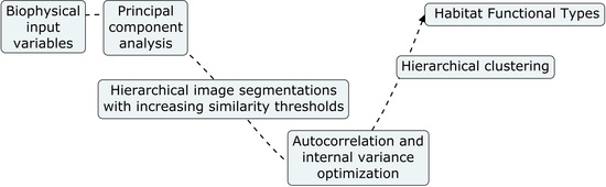
2. Methods
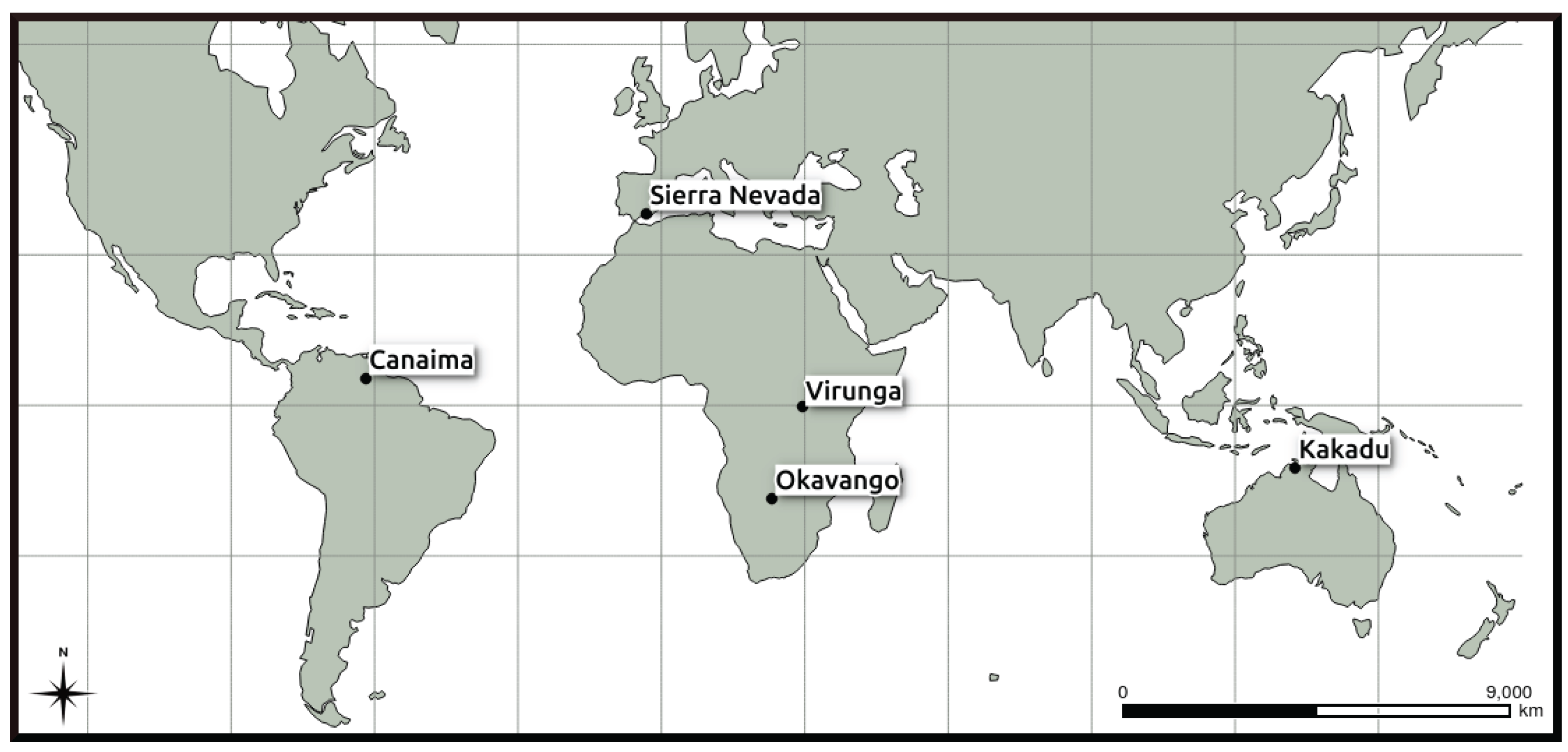
2.1. Study Area
2.2. Biophysical Input Variables
2.3. Retrieval of Habitat Functional Types
2.4. eHabitat+ Source Code
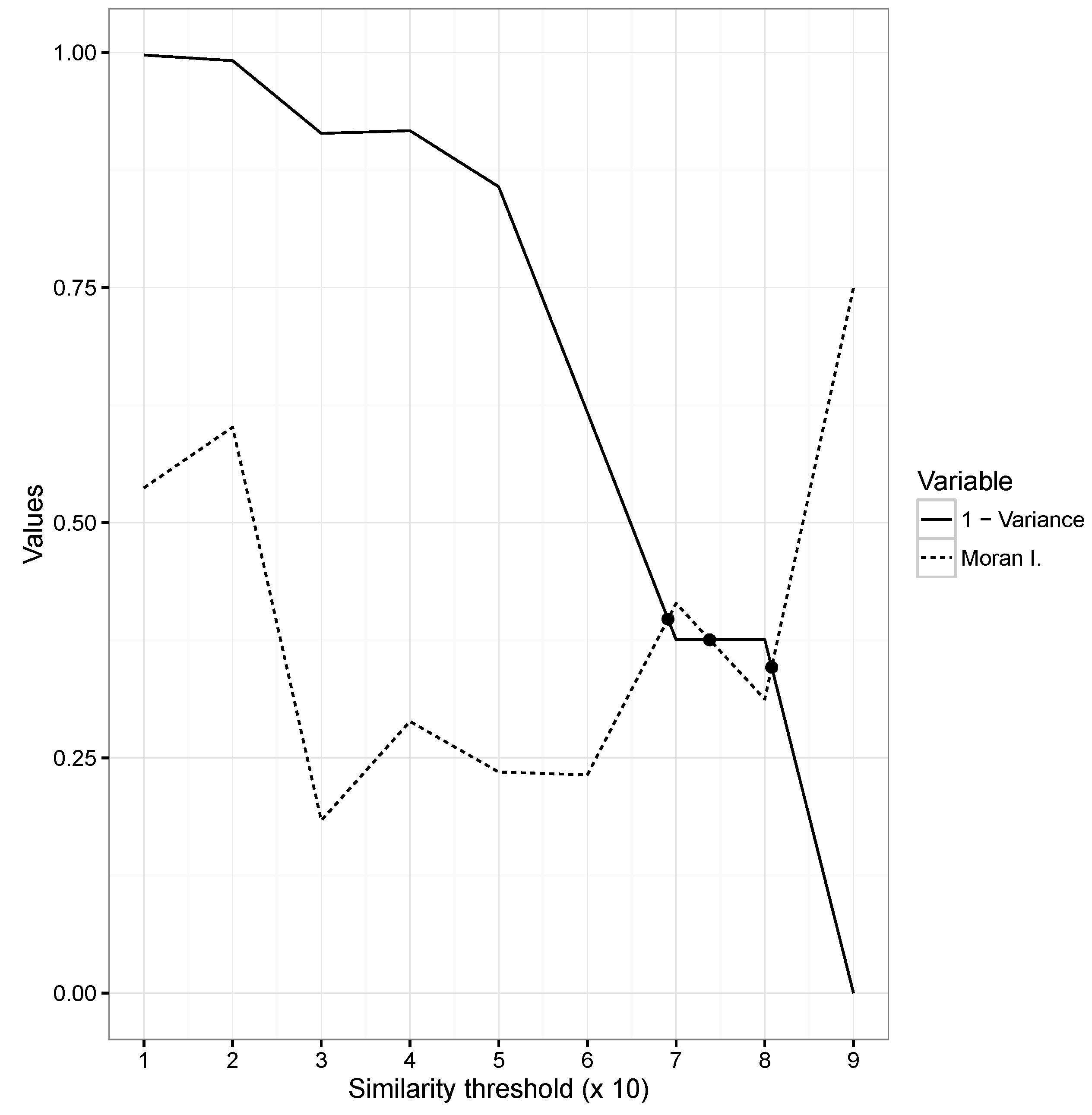
2.5. Evaluation and Assessment
3. Results
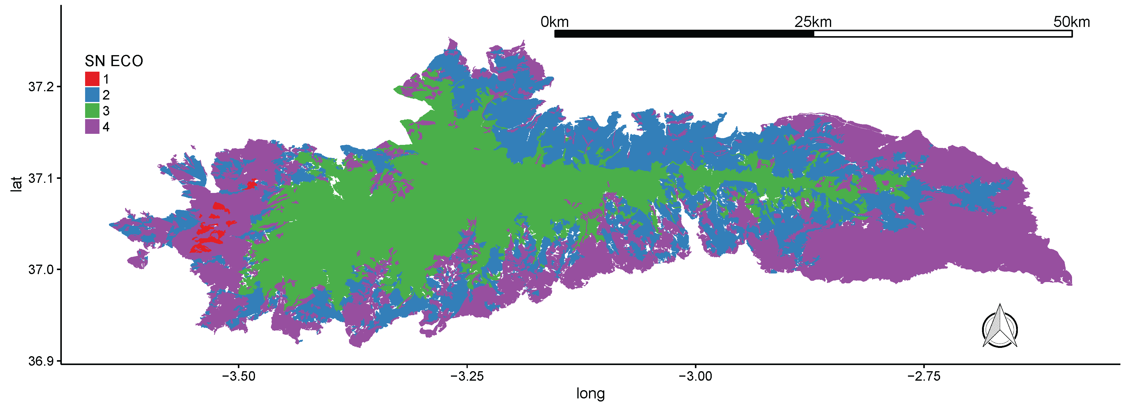
3.1. Sierra Nevada National Park
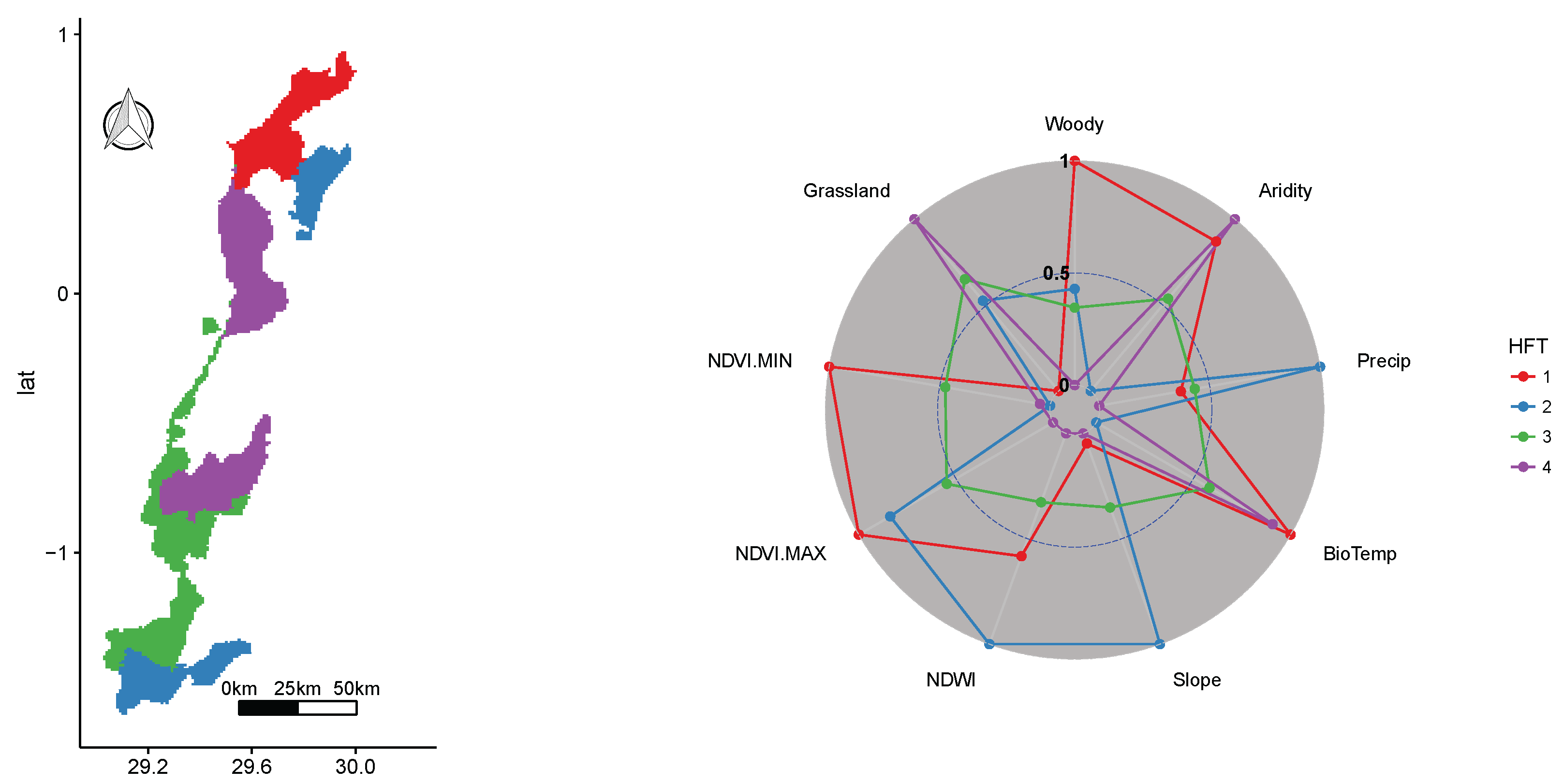
3.2. Virunga National Park WHS
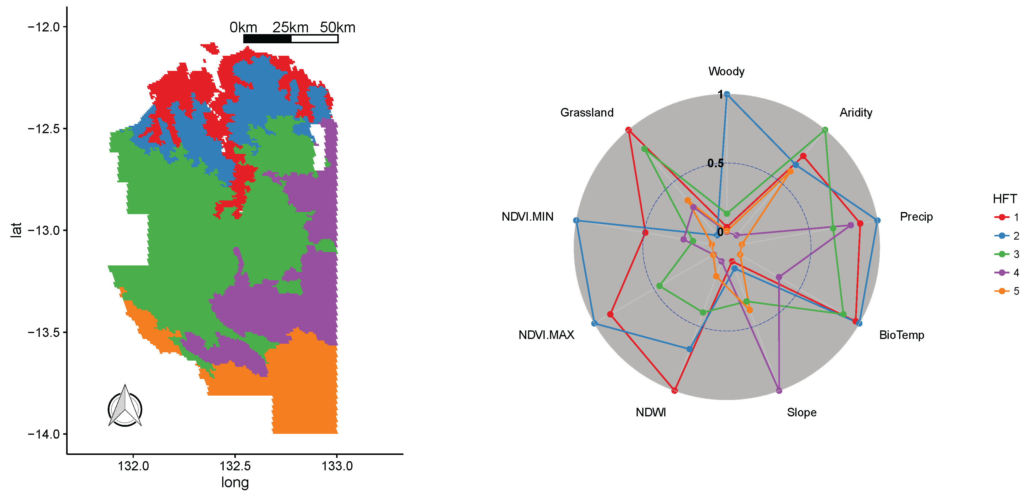
3.3. Kakadu National Park WHS
3.4. Okavango Delta WHS
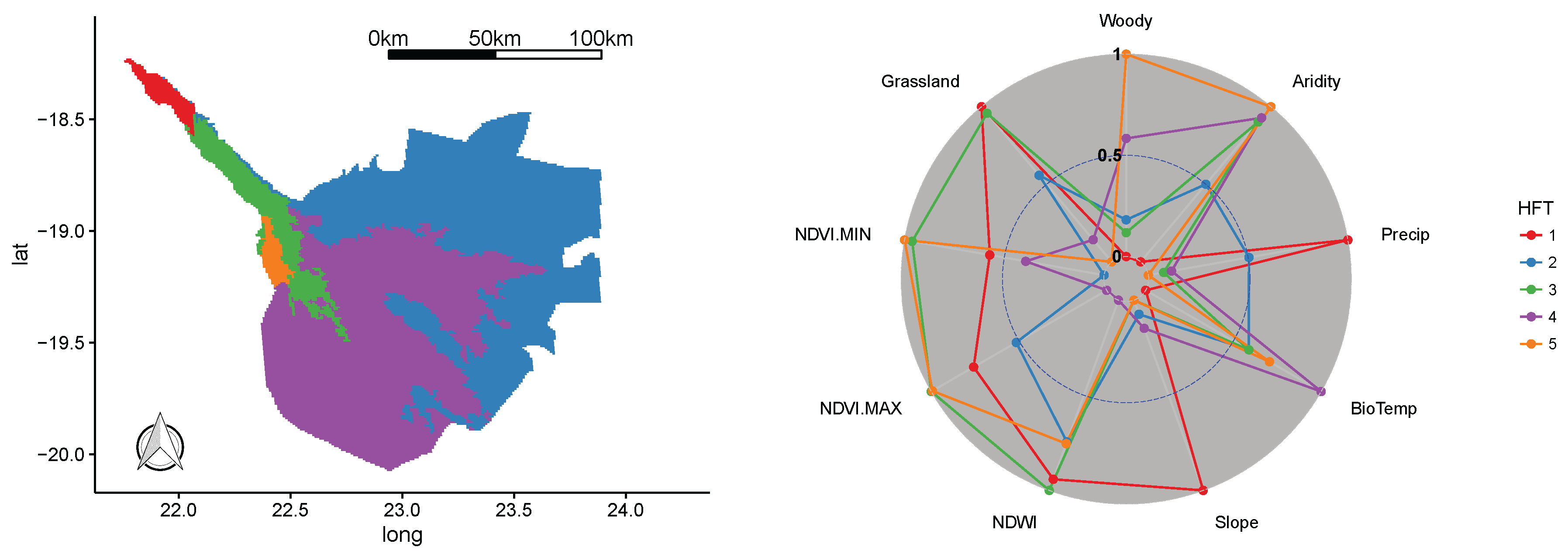
3.5. Canaima National Park WHS
3.6. Optimization and Input Variables

4. Discussion
5. Conclusions
Supplementary Materials
Acknowledgments
Author Contributions
Conflicts of Interest
References
- Watson, J.E.M.; Dudley, N.; Segan, D.B.; Hockings, M. The performance and potential of protected areas. Nature 2014, 515, 67–73. [Google Scholar] [CrossRef] [PubMed]
- Andam, K.S.; Ferraro, P.J.; Sims, K.R.E.; Healy, A.; Holland, M.B. Protected areas reduced poverty in Costa Rica and Thailand. Proc. Natl. Acad. Sci. USA 2010, 107, 9996–10001. [Google Scholar] [CrossRef] [PubMed]
- Ezebilo, E.E.; Mattsson, L. Socio-economic benefits of protected areas as perceived by local people around Cross River National Park, Nigeria. For. Policy Econ. 2010, 12, 189–193. [Google Scholar] [CrossRef]
- Juffe-Bignoli, D.; Burgess, N.; Bingham, H.; Belle, E.; de Lima, M.; Deguignet, M.; Bertzky, B.; Milam, A.; Martínez-López, J.; Lewis, E.; et al. Protected Planet Report 2014; UNEP-WCMC: Cambridge, UK, 2014. [Google Scholar]
- Jenkins, C.N.; Van Houtan, K.S.; Pimm, S.L.; Sexton, J.O. US protected lands mismatch biodiversity priorities. Proc. Natl. Acad. Sci. USA 2015, 112, 5081–5086. [Google Scholar] [CrossRef] [PubMed]
- Pressey, R.L.; Cabeza, M.; Watts, M.E.; Cowling, R.M.; Wilson, K.A. Conservation planning in a changing world. Trends Ecol. Evol. 2007, 22, 583–592. [Google Scholar] [CrossRef] [PubMed]
- International Union for Conservation of Nature (IUCN). Red List of Threatened Species, Version 2015-04. 2015. Available online: http://www.iucnredlist.org (accessed on 16 September 2016).
- Ceauşu, S.; Gomes, I.; Pereira, H.M. Conservation planning for biodiversity and wilderness: A real-world example. Environ. Manag. 2015, 55, 1168–1180. [Google Scholar] [CrossRef] [PubMed]
- Albuquerque, F.; Beier, P. Global patterns and environmental correlates of high-priority conservation areas for vertebrates. J. Biogeogr. 2015, 42, 1397–1405. [Google Scholar] [CrossRef]
- Possingham, H.P.; Andelman, S.J.; Burgman, M.A.; Medellín, R.A.; Master, L.L.; Keith, D.A. Limits to the use of threatened species lists. Trends Ecol. Evol. 2002, 17, 503–507. [Google Scholar] [CrossRef] [Green Version]
- Hartley, A.J.; Nelson, A.; Mayaux, P.; Grégoire, J.M. The Assessment of African Protected Areas; JRC Scientific and Technical Reports, EUR 21296 EN; Office for Official Publications of the European Communities: Luxembourg, 2007; p. 70. [Google Scholar]
- Jongman, R.H.G. Biodiversity observation from local to global. Ecol. Indic. 2013, 33, 1–4. [Google Scholar] [CrossRef]
- Buchanan, G.M.; Nelson, A.; Mayaux, P.; Hartley, A.; Donald, P.F. Delivering a global, terrestrial, biodiversity observation system through remote sensing. Conserv. Biol. 2009, 23, 499–502. [Google Scholar] [CrossRef] [PubMed]
- Evans, M.R. Modelling ecological systems in a changing world. Philos. Trans. R. Soc. Lond. B Biol. Sci. 2011, 367, 181–190. [Google Scholar] [CrossRef] [PubMed]
- Kuenzer, C.; Ottinger, M.; Wegmann, M.; Guo, H.; Wang, C.; Zhang, J.; Dech, S.; Wikelski, M. Earth observation satellite sensors for biodiversity monitoring: Potentials and bottlenecks. Int. J. Remote Sens. 2014, 35, 6599–6647. [Google Scholar] [CrossRef]
- Pettorelli, N.; Laurance, W.F.; O’Brien, T.G.; Wegmann, M.; Nagendra, H.; Turner, W. Satellite remote sensing for applied ecologists: Opportunities and challenges. J. Appl. Ecol. 2014, 51, 839–848. [Google Scholar] [CrossRef]
- Martínez-López, J.; Carreño, M.; Palazón-Ferrando, J.; Martínez-Fernández, J.; Esteve, M. Remote sensing of plant communities as a tool for assessing the condition of semiarid Mediterranean saline wetlands in agricultural catchments. Int. J. Appl. Earth Observ. Geoinf. 2014, 26, 193–204. [Google Scholar] [CrossRef]
- Lück-Vogel, M.; O’Farrell, P.J.; Roberts, W. Remote sensing based ecosystem state assessment in the Sandveld Region, South Africa. Ecol. Indic. 2013, 33, 60–70. [Google Scholar] [CrossRef]
- Rose, R.A.; Byler, D.; Eastman, J.R.; Fleishman, E.; Geller, G.; Goetz, S.; Guild, L.; Hamilton, H.; Hansen, M.; Headley, R.; et al. Ten ways remote sensing can contribute to conservation. Conserv. Biol. 2015, 29, 350–359. [Google Scholar] [CrossRef] [PubMed]
- Turner, W.; Rondinini, C.; Pettorelli, N.; Mora, B.; Leidner, A.K.; Szantoi, Z.; Buchanan, G.; Dech, S.; Dwyer, J.; Herold, M.; et al. Free and open-access satellite data are key to biodiversity conservation. Biol. Conserv. 2015, 182, 173–176. [Google Scholar] [CrossRef]
- Andrew, M.E.; Wulder, M.A.; Nelson, T.A. Potential contributions of remote sensing to ecosystem service assessments. Prog. Phys. Geogr. 2014, 38, 328–353. [Google Scholar] [CrossRef]
- Boykin, K.G.; Kepner, W.G.; Bradford, D.F.; Guy, R.K.; Kopp, D.A.; Leimer, A.K.; Samson, E.A.; East, N.F.; Neale, A.C.; Gergely, K.J. A national approach for mapping and quantifying habitat-based biodiversity metrics across multiple spatial scales. Ecol. Indic. 2013, 33, 139–147. [Google Scholar] [CrossRef]
- Chape, S.; Harrison, J.; Spalding, M.; Lysenko, I. Measuring the extent and effectiveness of protected areas as an indicator for meeting global biodiversity targets. Philos. Trans. R. Soc. B Biol. Sci. 2005, 360, 443–455. [Google Scholar] [CrossRef] [PubMed]
- Bunce, R.G.H.; Bogers, M.M.B.; Evans, D.; Halada, L.; Jongman, R.H.G.; Mucher, C.A.; Bauch, B.; de Blust, G.; Parr, T.W.; Olsvig-Whittaker, L. The significance of habitats as indicators of biodiversity and their links to species. Ecol. Indic. 2013, 33, 19–25. [Google Scholar] [CrossRef]
- Eigenbrod, F.; Gonzalez, P.; Dash, J.; Steyl, I. Vulnerability of ecosystems to climate change moderated by habitat intactness. Glob. Chang. Biol. 2015, 21, 275–286. [Google Scholar] [CrossRef] [PubMed]
- Butchart, S.H.; Clarke, M.; Smith, R.J.; Sykes, R.E.; Scharlemann, J.P.; Harfoot, M.; Buchanan, G.M.; Angulo, A.; Balmford, A.; Bertzky, B.; et al. Shortfalls and solutions for meeting national and global conservation area targets. Conserv. Lett. 2015, 8, 329–337. [Google Scholar] [CrossRef]
- Dubois, G.; Schulz, M.; Skøien, J.; Cottam, A.; Temperley, W.; Clerici, M.; Drakou, E.; van’t Klooster, J.; Verbeeck, B.; Palumbo, I.; et al. An Introduction to the Digital Observatory for Protected Areas (DOPA) and the DOPA Explorer (Beta); EUR 26207 EN; Publications Office of the European Union: Luxembourg, 2013; p. 71. [Google Scholar]
- Dubois, G.; Bastin, L.; Martínez-López, J.; Cottam, A.; Temperley, W.; Bertzky, B.; Graziano, M. The Digital Observatory for Protected Areas (DOPA) Explorer 1.0; EUR 27162 EN; Publications Office of the European Union: Luxembourg, 2015; p. 53. [Google Scholar]
- Dubois, G.; Schulz, M.; Skøien, J.; Bastin, L.; Peedell, S. eHabitat, a multi-purpose Web Processing Service for ecological modelling. Environ. Model. Softw. 2013, 41, 123–133. [Google Scholar] [CrossRef]
- IUCN and UNEP-WCMC. The World Database on Protected Areas (WDPA); UNEP World Conservation Monitoring Centre: Cambridge, UK, 2016. [Google Scholar]
- International Union for Conservation of Nature (IUCN). Habitats Classification Scheme, Version 3.1; IUCN: Cambridge, UK, 2012. [Google Scholar]
- Council of Europe. Council Directive 92/43/EEC of 21 May 1992 on the Conservation of Natural Habitats and of Wild Fauna and Flora; Council of Europe: Strasbourg, France, 1992. [Google Scholar]
- Hortal, J.; Triantis, K.; Meiri, S.; Thébault, E.; Sfenthourakis, S. Island species richness increases with habitat diversity. Am. Nat. 2009, 174, E205–E217. [Google Scholar] [CrossRef] [PubMed]
- Nieto, S.; Flombaum, P.; Garbulsky, M.F. Can temporal and spatial NDVI predict regional bird-species richness? Glob. Ecol. Conserv. 2015, 3, 729–735. [Google Scholar] [CrossRef] [Green Version]
- Debinski, D.M.; Kindscher, K.; Jakubauskas, M.E. A remote sensing and GIS-based model of habitats and biodiversity in the Greater Yellowstone Ecosystem. Int. J. Remote Sens. 1999, 20, 3281–3291. [Google Scholar] [CrossRef]
- Borre, J.V.; Paelinckx, D.; Mücher, C.A.; Kooistra, L.; Haest, B.; Blust, G.D.; Schmidt, A.M. Integrating remote sensing in Natura 2000 habitat monitoring: Prospects on the way forward. J. Nat. Conserv. 2011, 19, 116–125. [Google Scholar] [CrossRef]
- Ekroos, J.; Kuussaari, M.; Tiainen, J.; Heliölä, J.; Seimola, T.; Helenius, J. Correlations in species richness between taxa depend on habitat, scale and landscape context. Ecol. Indic. 2013, 34, 528–535. [Google Scholar] [CrossRef]
- Kerr, J.T.; Ostrovsky, M. From space to species: ecological applications for remote sensing. Trends Ecol. Evol. 2003, 18, 299–305. [Google Scholar] [CrossRef]
- Durant, S.M.; Wacher, T.; Bashir, S.; Woodroffe, R.; De Ornellas, P.; Ransom, C.; Newby, J.; Abáigar, T.; Abdelgadir, M.; El Alqamy, H.; et al. Fiddling in biodiversity hotspots while deserts burn? Collapse of the Sahara’s megafauna. Divers. Distrib. 2014, 20, 114–122. [Google Scholar] [CrossRef]
- Keith, D.A.; Rodríguez, J.P.; Brooks, T.M.; Burgman, M.A.; Barrow, E.G.; Bland, L.; Comer, P.J.; Franklin, J.; Link, J.; McCarthy, M.A.; et al. The IUCN Red List of Ecosystems: Motivations, challenges and applications. Conserv. Lett. 2015, 8, 214–226. [Google Scholar] [CrossRef]
- Wilson, M.; Chen, X.Y.; Corlett, R.; Didham, R.; Ding, P.; Holt, R.; Holyoak, M.; Hu, G.; Hughes, A.; Jiang, L.; et al. Habitat fragmentation and biodiversity conservation: Key findings and future challenges. Landsc. Ecol. 2016, 31, 219–227. [Google Scholar] [CrossRef]
- Van der Hoek, Y.; Zuckerberg, B.; Manne, L.L. Application of habitat thresholds in conservation: Considerations, limitations, and future directions. Glob. Ecol. Conserv. 2015, 3, 736–743. [Google Scholar] [CrossRef]
- Alcaraz, D.; Paruelo, J.; Cabello, J. Identification of current ecosystem functional types in the Iberian Peninsula. Glob. Ecol. Biogeogr. 2006, 15, 200–212. [Google Scholar] [CrossRef]
- Gauthier, P.; Foulon, Y.; Jupille, O.; Thompson, J.D. Quantifying habitat vulnerability to assess species priorities for conservation management. Biol. Conserv. 2013, 158, 321–325. [Google Scholar] [CrossRef]
- Geldmann, J.; Barnes, M.; Coad, L.; Craigie, I.D.; Hockings, M.; Burgess, N.D. Effectiveness of terrestrial protected areas in reducing habitat loss and population declines. Biol. Conserv. 2013, 161, 230–238. [Google Scholar] [CrossRef]
- Keith, D.A.; Rodríguez, J.P.; Rodríguez-Clark, K.M.; Nicholson, E.; Aapala, K.; Alonso, A.; Asmussen, M.; Bachman, S.; Basset, A.; Barrow, E.G.; et al. Scientific Foundations for an IUCN Red List of Ecosystems. PLoS ONE 2013, 8, e62111. [Google Scholar] [CrossRef] [PubMed] [Green Version]
- Host, G.E.; Polzer, P.L.; Mladenoff, D.J.; White, M.A.; Crow, T.R. A quantitative approach to developing regional ecosystem classifications. Ecol. Appl. 1996, 6, 608–618. [Google Scholar] [CrossRef]
- Olson, D.M.; Dinerstein, E.; Wikramanayake, E.D.; Burgess, N.D.; Powell, G.V.N.; Underwood, E.C.; D’amico, J.A.; Itoua, I.; Strand, H.E.; Morrison, J.C.; et al. Terrestrial ecoregions of the world: A new map of life on earth: A new global map of terrestrial ecoregions provides an innovative tool for conserving biodiversity. BioScience 2001, 51, 933–938. [Google Scholar] [CrossRef]
- Pérez-Hoyos, A.; Martínez, B.; García-Haro, F.J.; Moreno, A.; Gilabert, M.A. Identification of ecosystem functional types from coarse resolution imagery using a self-organizing map approach: A case study for Spain. Remote Sens. 2014, 6, 11391–11419. [Google Scholar] [CrossRef]
- Pettorelli, N.; Chauvenet, A.L.; Duffy, J.P.; Cornforth, W.A.; Meillere, A.; Baillie, J.E. Tracking the effect of climate change on ecosystem functioning using protected areas: Africa as a case study. Ecol. Indic. 2012, 20, 269–276. [Google Scholar] [CrossRef]
- Paruelo, M.J.; Jobbágy, G.E.; Sala, E.O. Current distribution of ecosystem functional types in temperate South America. Ecosystems 2001, 4, 683–698. [Google Scholar] [CrossRef]
- Ivits, E.; Cherlet, M.; Mehl, W.; Sommer, S. Ecosystem functional units characterized by satellite observed phenology and productivity gradients: A case study for Europe. Ecol. Indic. 2013, 27, 17–28. [Google Scholar] [CrossRef]
- DOPA Wiki. Habitat Functional Types. 2016. Available online: https://dopa.wikispaces.com/Habitat+Functional+Types (accessed on 16 September 2016).
- IUCN and UNEP-WCMC. The World Database on Protected Areas (WDPA); UNEP World Conservation Monitoring Centre: Cambridge, UK, 2014. [Google Scholar]
- Drakou, E.G.; Kallimanis, A.S.; Mazaris, A.D.; Apostolopoulou, E.; Pantis, J.D. Habitat type richness associations with environmental variables: A case study in the Greek Natura 2000 aquatic ecosystems. Biodivers. Conserv. 2011, 20, 929–943. [Google Scholar] [CrossRef]
- Skøien, J.O.; Schulz, M.; Dubois, G.; Fisher, I.; Balman, M.; May, I.; Tuama, E.O. A Model Web approach to modelling climate change in biomes of Important Bird Areas. Ecol. Inform. 2013, 14, 38–43. [Google Scholar] [CrossRef]
- Metzger, M.J.; Bunce, R.G.H.; Jongman, R.H.G.; Muecher, C.A.; Watkins, J.W. A climatic stratification of the environment of Europe. Glob. Ecol. Biogeogr. 2005, 14, 549–563. [Google Scholar] [CrossRef]
- Metzger, M.J.; Bunce, R.G.H.; Jongman, R.H.G.; Sayre, R.; Trabucco, A.; Zomer, R. A high-resolution bioclimate map of the world: A unifying framework for global biodiversity research and monitoring. Glob. Ecol. Biogeogr. 2013, 22, 630–638. [Google Scholar] [CrossRef]
- Ortega, M.; Guerra, C.; Honrado, J.P.; Metzger, M.J.; Bunce, R.G.H.; Jongman, R.H.G. Surveillance of habitats and plant diversity indicators across a regional gradient in the Iberian Peninsula. Ecol. Indic. 2013, 33, 36–44. [Google Scholar] [CrossRef] [Green Version]
- Metzger, M.J.; Brus, D.J.; Bunce, R.G.H.; Carey, P.D.; Gonçalves, J.; Honrado, J.P.; Jongman, R.H.G.; Trabucco, A.; Zomer, R. Environmental stratifications as the basis for national, European and global ecological monitoring. Ecol. Indic. 2013, 33, 26–35. [Google Scholar] [CrossRef]
- Farr, T.G.; Rosen, P.A.; Caro, E.; Crippen, R.; Duren, R.; Hensley, S.; Kobrick, M.; Paller, M.; Rodriguez, E.; Roth, L.; et al. The shuttle radar topography mission. Rev. Geophys. 2007, 45, RG2004. [Google Scholar] [CrossRef]
- Hijmans, R.J.; Cameron, S.E.; Parra, J.L.; Jones, P.G.; Jarvis, A. Very high resolution interpolated climate surfaces for global land areas. Int. J. Climatol. 2005, 25, 1965–1978. [Google Scholar] [CrossRef]
- DiMiceli, C.; Carroll, M.; Sohlberg, R.; Huang, C.; Hansen, M.; Townshend, J.R.G. Annual Global Automated MODIS Vegetation Continuous Fields (MOD44B) at 250 m Spatial Resolution for Data Years Beginning Day 65, 2000–2010, Collection 5 Percent Tree Cover; University of Maryland: College Park, MD, USA, 2011. [Google Scholar]
- Rouse, J.W.; Haas, R.H.; Schell, J.A.; Deering, D.W. Monitoring vegetation systems in the Great Plains with ERTS. In Proceedings of the Third ERTS Symposium (NASA), Washington, DC, USA, 10–14 December 1973; Volume 1, pp. 309–317.
- Carroll, M.; DiMiceli, C.; Sohlberg, R.; Townshend, J. 250 m MODIS Normalized Difference Vegetation Index; University of Maryland: College Park, MD, USA, 2004. [Google Scholar]
- Pettorelli, N.; Vik, J.O.; Mysterud, A.; Gaillard, J.M.; Tucker, C.J.; Stenseth, N.C. Using the satellite-derived NDVI to assess ecological responses to environmental change. Trends Ecol. Evol. 2005, 20, 503–510. [Google Scholar] [CrossRef] [PubMed]
- Tucker, C.J. Remote sensing of leaf water content in the near infrared. Remote Sens. Environ. 1980, 10, 23–32. [Google Scholar] [CrossRef]
- Dong, Z.; Wang, Z.; Liu, D.; Li, L.; Ren, C.; Tang, X.; Jia, M.; Liu, C. Assessment of habitat suitability for water birds in the West Songnen Plain, China, using remote sensing and GIS. Ecol. Eng. 2013, 55, 94–100. [Google Scholar] [CrossRef]
- Stow, D.; Hamada, Y.; Coulter, L.; Anguelova, Z. Monitoring shrubland habitat changes through object-based change identification with airborne multispectral imagery. Remote Sens. Environ. 2008, 112, 1051–1061. [Google Scholar] [CrossRef]
- Hasan, R.C.; Ierodiaconou, D.; Laurenson, L. Combining angular response classification and backscatter imagery segmentation for benthic biological habitat mapping. Estuar. Coast. Shelf Sci. 2012, 97, 1–9. [Google Scholar] [CrossRef] [Green Version]
- Bock, M.; Xofis, P.; Mitchley, J.; Rossner, G.; Wissen, M. Object-oriented methods for habitat mapping at multiple scales—Case studies from Northern Germany and Wye Downs, UK. J. Nat. Conserv. 2005, 13, 75–89. [Google Scholar] [CrossRef]
- Micallef, A.; Bas, T.P.L.; Huvenne, V.A.; Blondel, P.; Hühnerbach, V.; Deidun, A. A multi-method approach for benthic habitat mapping of shallow coastal areas with high-resolution multibeam data. Cont. Shelf Res. 2012, 39–40, 14–26. [Google Scholar] [CrossRef] [Green Version]
- Blaschke, T. Object based image analysis for remote sensing. ISPRS J. Photogramm. Remote Sens. 2010, 65, 2–16. [Google Scholar] [CrossRef]
- Carleer, A.; Debeir, O.; Wolff, E. Assessment of Very High Spatial Resolution Satellite Image Segmentations. Photogramm. Eng. Remote Sens. 2005, 71, 1285–1294. [Google Scholar] [CrossRef]
- Adams, R.; Bischof, L. Seeded region growing. IEEE Trans. Pattern Anal. Mach. Intell. 1994, 16, 641–647. [Google Scholar] [CrossRef]
- Fonseca, L.M.G.; Ii, F.M. Satellite imagery segmentation: A region growing approach. In Proceeedings of the VIII Brazilian Symposium on Remote Sensing, Salvador, Brazil, 14–19 April 1996; pp. 677–680.
- Cheng, H.; Jiang, X.; Sun, Y.; Wang, J. Color image segmentation: advances and prospects. Pattern Recognit. 2001, 34, 2259–2281. [Google Scholar] [CrossRef]
- Momsen, E.; Metz, M. I.segment Manual—Identifies Segments (Objects) from Imagery Data. 2016. Available online: https://grass.osgeo.org/grass73/manuals/i.segment.html (accessed on 16 September 2016).
- Espindola, G.M.; Camara, G.; Reis, I.A.; Bins, L.S.; Monteiro, A.M. Parameter selection for region-growing image segmentation algorithms using spatial autocorrelation. Int. J. Remote Sens. 2006, 27, 3035–3040. [Google Scholar] [CrossRef]
- Cánovas-García, F.; Alonso-Sarría, F. A local approach to optimize the scale parameter in multiresolution segmentation for multispectral imagery. Geocarto Int. 2015, 30, 937–961. [Google Scholar] [CrossRef]
- Johnson, B.; Xie, Z. Unsupervised image segmentation evaluation and refinement using a multi-scale approach. ISPRS J. Photogramm. Remote Sens. 2011, 66, 473–483. [Google Scholar] [CrossRef]
- Johnston, C.A.; Zedler, J.B.; Tulbure, M.G.; Frieswyk, C.B.; Bedford, B.L.; Vaccaro, L. A unifying approach for evaluating the condition of wetland plant communities and identifying related stressors. Ecol. Appl. 2009, 19, 1739–1757. [Google Scholar] [CrossRef] [PubMed]
- Rocchini, D.; Foody, G.M.; Nagendra, H.; Ricotta, C.; Anand, M.; He, K.S.; Amici, V.; Kleinschmit, B.; Förster, M.; Schmidtlein, S.; et al. Uncertainty in ecosystem mapping by remote sensing. Comput. Geosci. 2013, 50, 128–135. [Google Scholar] [CrossRef]
- Neteler, M.; Bowman, M.H.; Landa, M.; Metz, M. GRASS GIS: A multi-purpose open source GIS. Environ. Model. Softw. 2012, 31, 124–130. [Google Scholar] [CrossRef]
- Van Rossum, G.; Drake, F.L. Python Language Reference Manual, Version 2.7; Available online: https://docs.python.org/2/reference/ (accessed on 16 September 2016).
- R Core Team. R: A Language and Environment for Statistical Computing; R Foundation for Statistical Computing: Vienna, Austria, 2012. [Google Scholar]
- Martínez-López, J. eHabitat+ Source Code for DOPA. 2016. Available online: http://0-dx-doi-org.brum.beds.ac.uk/10.5281/zenodo.51879 (accessed on 16 September 2016).
- Bennett, N.D.; Croke, B.F.; Guariso, G.; Guillaume, J.H.; Hamilton, S.H.; Jakeman, A.J.; Marsili-Libelli, S.; Newham, L.T.; Norton, J.P.; Perrin, C.; et al. Characterising performance of environmental models. Environ. Model. Softw. 2013, 40, 1–20. [Google Scholar] [CrossRef]
- Li, Z.; Xu, D.; Guo, X. Remote sensing of ecosystem health: Opportunities, challenges, and future perspectives. Sensors 2014, 14, 21117–21139. [Google Scholar] [CrossRef] [PubMed]
- Oksanen, J.; Blanchet, F.G.; Kindt, R.; Legendre, P.; Minchin, P.R.; O’Hara, R.B.; Simpson, G.L.; Solymos, P.; Stevens, M.H.H.; Wagner, H. Vegan: Community Ecology Package, R package version 2.3–3. 2016. Available online: https://cran.r-project.org/web/packages/vegan/index.html (accessed on 16 September 2016).
- Martínez-López, J.; Martínez-Fernández, J.; Naimi, B.; Carreño, M.F.; Esteve, M.A. An open-source spatio-dynamic wetland model of plant community responses to hydrological pressures. Ecol. Model. 2015, 306, 326–333. [Google Scholar] [CrossRef]
- Kuhnert, M.; Voinov, A.; Seppelt, R. Comparing raster map comparison algorithms for spatial modelling and analysis. Photogramm. Eng. Remote Sens. 2005, 71, 975–984. [Google Scholar] [CrossRef]
- Costanza, R. Model goodness of fit: A multiple resolution procedure. Ecol. Model. 1989, 47, 199–215. [Google Scholar] [CrossRef]
- Bonet, F.; Pérez-Luque, A.; Moreno, R.; Zamora, R. Sierra Nevada Global Change Observatory. Structure and Basic Data; Environment Department (Andalusian Regional Government)—University of Granada: Granada, Spain, 2010; p. 48.
- Aspizua, R.; Bonet, F.; Zamora, R.; Sánchez, F.; Cano-Manuel, F.; Henares, I. El observatorio de cambio global de Sierra Nevada: Hacia la gestión adaptativa de los espacios naturales. Rev. Ecosyst. 2010, 19, 56–68. [Google Scholar]
- UNESCO. World Heritage Nomination for Virunga National Park—Vegetation Map. 1979. Available online: http://whc.unesco.org/en/list/63/documents/ (accessed on 16 September 2016).
- Bastin, G.; ACRIS Management Committee. Rangelands 2008: Taking the Pulse; National Land and Water Resources Audit: Canberra, Australia, 2008. [Google Scholar]
- Mendelsohn, J.; van der Post, C.; Ramberg, L.; Murray-Hudson, M.; Wolski, P.; Mosepele, K. Okavango Delta: Floods of Life; Raison: Windhoek, Namibia; Island Press: Washington, DC, USA, 2010. [Google Scholar]
- Delgado, L.; Castellanos, H.; Rodríguez, M. Vegetación del parque nacional canaima. In Biodiversidad del Parque Nacional Canaima: Bases Técnicas Para la Conservacion de la Guayana Venezolana; Señaris, J.C., Lew, D., Lasso, C.A., Eds.; Fundación La Salle de Ciencias Naturales and The Nature Conservancy: Caracas, Venezuela, 2009; pp. 39–73. [Google Scholar]
- Hortal, J.; Carrascal, L.M.; Triantis, K.A.; Thébault, E.; Meiri, S.; Sfenthourakis, S. Species richness can decrease with altitude but not with habitat diversity. Proc. Natl. Acad. Sci. USA 2013, 110, E2149–E2150. [Google Scholar] [CrossRef] [PubMed]
- Marchese, C. Biodiversity hotspots: A shortcut for a more complicated concept. Glob. Ecol. Conserv. 2015, 3, 297–309. [Google Scholar] [CrossRef]
- Estreguil, C.; Rigo, D.D.; Caudullo, G. A proposal for an integrated modelling framework to characterise habitat pattern. Environ. Model. Softw. 2014, 52, 176–191. [Google Scholar] [CrossRef]
- Jenkins, C.N.; Joppa, L. Expansion of the global terrestrial protected area system. Biol. Conserv. 2009, 142, 2166–2174. [Google Scholar] [CrossRef]
- Pascual-Hortal, L.; Saura, S. Comparison and development of new graph-based landscape connectivity indices: Towards the priorization of habitat patches and corridors for conservation. Landsc. Ecol. 2006, 21, 959–967. [Google Scholar] [CrossRef]
- Santini, L.; Saura, S.; Rondinini, C. Connectivity of the global network of protected areas. Divers. Distrib. 2015, 24, 2405. [Google Scholar] [CrossRef]
- Cabeza, M.; Moilanen, A. Design of reserve networks and the persistence of biodiversity. Trends Ecol. Evol. 2001, 16, 242–248. [Google Scholar] [CrossRef]
- Müller, O.V.; Berbery, E.H.; Alcaraz-Segura, D.; Ek, M.B. Regional model simulations of the 2008 drought in southern South America using a consistent set of land surface properties. J. Clim. 2014, 27, 6754–6778. [Google Scholar] [CrossRef]
- Lee, S.J.; Berbery, E.H.; Alcaraz-Segura, D. The impact of ecosystem functional type changes on the La Plata Basin climate. Adv. Atmos. Sci. 2013, 30, 1387–1405. [Google Scholar] [CrossRef]
- Villa, F.; Bagstad, K.J.; Voigt, B.; Johnson, G.W.; Portela, R.; Honzák, M.; Batker, D. A methodology for adaptable and robust ecosystem services assessment. PLoS ONE 2014, 9, e91001. [Google Scholar] [CrossRef] [PubMed]
- Ivits, E.; Cherlet, M.; Horion, S.; Fensholt, R. Global biogeographical pattern of ecosystem functional types derived from earth observation data. Remote Sens. 2013, 5, 3305–3330. [Google Scholar] [CrossRef]
- Corbane, C.; Lang, S.; Pipkins, K.; Alleaume, S.; Deshayes, M.; Millán, V.E.G.; Strasser, T.; Borre, J.V.; Toon, S.; Michael, F. Remote sensing for mapping natural habitats and their conservation status—New opportunities and challenges. Int. J. Appl. Earth Observ. Geoinf. 2015, 37, 7–16. [Google Scholar] [CrossRef]
- Drielsma, M.; Ferrier, S.; Howling, G.; Manion, G.; Taylor, S.; Love, J. The Biodiversity Forecasting Toolkit: Answering the ’how much’, ’what’, and ’where’ of planning for biodiversity persistence. Ecol. Model. 2014, 274, 80–91. [Google Scholar] [CrossRef]
- Giri, C.; Ochieng, E.; Tieszen, L.L.; Zhu, Z.; Singh, A.; Loveland, T.; Masek, J.; Duke, N. Status and distribution of mangrove forests of the world using earth observation satellite data. Glob. Ecol. Biogeogr. 2011, 20, 154–159. [Google Scholar] [CrossRef]
- Hobern, D.; Apostolico, A.; Arnaud, E.; Bello, J.C.; Canhos, D.; Dubois, G.; Field, D.; Alonso Garcia, E.; Hardisty, A.; Harrison, J.; et al. Global Biodiversity Informatics Outlook: Delivering Biodiversity Knowledge in the Information Age; GBIF Secretariat: Copenhagen, Denmark, 2013. [Google Scholar]
- Martínez-López, J.; Carreño, M.F.; Palazón-Ferrando, J.A.; Martínez-Fernández, J.; Esteve, M.A. Free advanced modelling and remote-sensing techniques for wetland watershed delineation and monitoring. Int. J. Geogr. Inf. Sci. 2014, 28, 1610–1625. [Google Scholar] [CrossRef]
- Steiniger, S.; Hay, G.J. Free and open source geographic information tools for landscape ecology. Ecol. Inf. 2009, 4, 183–195. [Google Scholar] [CrossRef]


| PA Name | Country | Area (km2) | Date of Establishment | Key Biodiversity Values |
|---|---|---|---|---|
| Sierra Nevada National Park | Spain | 1724 | 2002 | Key biodiversity hotspot in the Mediterranean region. This PA harbours 27 habitat types (EU Habitats Directive), hosts 20% of the European flora, a high number of flora endemic species as well as a rich cultural heritage (90,000 people live inside the protected area). |
| Virunga National Park WHS | Democratic Republic of the Congo | 7805 | 1979 | Africa’s most diverse PA in terms of species and habitats, over 200 land mammals and over 700 bird species, many endemic species and |
| Kakadu National Park WHS | Australia | 19,139 | 1981 | Australia’s largest and most diverse National Park, great habitat diversity, supports over one third of Australia’s bird species and one quarter of Australia’s land mammals, many endemic species and water birds. |
| Okavango Delta WHS | Botswana | 20,443 | 2014 | Africa’s largest inland delta, unique hydrology, high habitat diversity, 130 land mammals and 480 bird species, including 24 species of globally-threatened birds, large populations of rhinos, elephants and water birds. |
| Canaima National Park WHS | Venezuela | 28,828 | 1994 | Unique table-mountain (Tepuis) landscape, high habitat and species diversity, many endemic species and migratory birds. |
| PA | Axis | Precipitation | Aridity | Slope | Woody | Grassland | NDWI | NDVI-MAX | NDVI-MIN | Bio-Temperature | Variance (%) |
|---|---|---|---|---|---|---|---|---|---|---|---|
| Sierra Nevada | PC1 | 0.3798 | −0.4652 | 0.1128 | 0.363 | 0.2713 | 0.2889 | 0.5039 | 0.2693 | −0.1062 | 37.92% |
| PC2 | −0.3683 | −0.1621 | 0.1251 | −0.2461 | 0.2237 | 0.4677 | −0.028 | −0.3868 | −0.5853 | 23.88% | |
| PC3 | 0.1043 | 0.098 | 0.5598 | 0.4198 | −0.6284 | 0.1423 | −0.1525 | −0.0939 | −0.2067 | 13.77% | |
| Virunga | PC1 | 0.1691 | 0.0572 | −0.1102 | 0.4964 | −0.4999 | 0.2782 | 0.4624 | 0.3513 | 0.2123 | 36.55% |
| PC2 | −0.4706 | 0.5499 | −0.3951 | −0.0085 | 0.0289 | −0.2638 | −0.0703 | 0.0721 | 0.4893 | 33.37% | |
| PC3 | −0.0333 | 0.0091 | −0.1165 | 0.3975 | −0.3685 | 0.0932 | −0.3242 | −0.76 | 0.0081 | 9.43% | |
| Kakadu | PC1 | 0.2659 | 0.3205 | −0.1959 | 0.1793 | 0.2094 | 0.4467 | 0.4678 | 0.2299 | 0.4908 | 36.49% |
| PC2 | −0.253 | 0.3062 | −0.2074 | −0.5443 | 0.5466 | 0.0878 | −0.1171 | −0.4244 | 0.0504 | 22.78% | |
| PC3 | 0.6715 | −0.5045 | 0.2479 | −0.3629 | 0.2778 | 0.0542 | −0.0859 | −0.0134 | 0.1175 | 13.20% | |
| Okavango | PC1 | 0.5353 | −0.5466 | 0.067 | −0.0024 | 0.2327 | 0.1736 | 0.2303 | −0.0723 | −0.5173 | 33.59% |
| PC2 | −0.0971 | 0.1109 | −0.0621 | −0.6826 | 0.5594 | 0.1382 | 0.0033 | −0.3986 | 0.1325 | 20.26% | |
| PC3 | −0.1693 | 0.1563 | −0.2218 | 0.1628 | 0.1822 | 0.5707 | 0.6151 | 0.3422 | 0.1297 | 17.71% | |
| Canaima | PC1 | 0.2057 | 0.0205 | 0.0303 | 0.4673 | −0.4632 | 0.4003 | 0.4509 | 0.3083 | 0.2545 | 46.11% |
| PC2 | −0.4905 | 0.7126 | −0.3334 | −0.0168 | 0.0164 | 0.1195 | −0.0196 | −0.0526 | 0.35 | 20.65% | |
| PC3 | −0.4288 | 0.0916 | 0.5272 | 0.1372 | −0.1333 | 0.2833 | 0.1727 | −0.4482 | −0.4269 | 17.35% |
© 2016 by the authors; licensee MDPI, Basel, Switzerland. This article is an open access article distributed under the terms and conditions of the Creative Commons Attribution (CC-BY) license (http://creativecommons.org/licenses/by/4.0/).
Share and Cite
Martínez-López, J.; Bertzky, B.; Bonet-García, F.J.; Bastin, L.; Dubois, G. Biophysical Characterization of Protected Areas Globally through Optimized Image Segmentation and Classification. Remote Sens. 2016, 8, 780. https://0-doi-org.brum.beds.ac.uk/10.3390/rs8090780
Martínez-López J, Bertzky B, Bonet-García FJ, Bastin L, Dubois G. Biophysical Characterization of Protected Areas Globally through Optimized Image Segmentation and Classification. Remote Sensing. 2016; 8(9):780. https://0-doi-org.brum.beds.ac.uk/10.3390/rs8090780
Chicago/Turabian StyleMartínez-López, Javier, Bastian Bertzky, Francisco Javier Bonet-García, Lucy Bastin, and Grégoire Dubois. 2016. "Biophysical Characterization of Protected Areas Globally through Optimized Image Segmentation and Classification" Remote Sensing 8, no. 9: 780. https://0-doi-org.brum.beds.ac.uk/10.3390/rs8090780