
Ground-Control Networks for Image Based Surface Reconstruction: An Investigation of Optimum Survey Designs Using UAV Derived Imagery and Structure-from-Motion Photogrammetry

Abstract
:1. Introduction
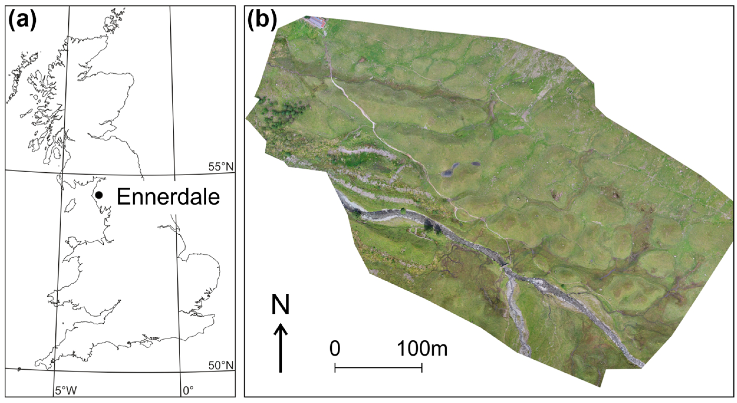
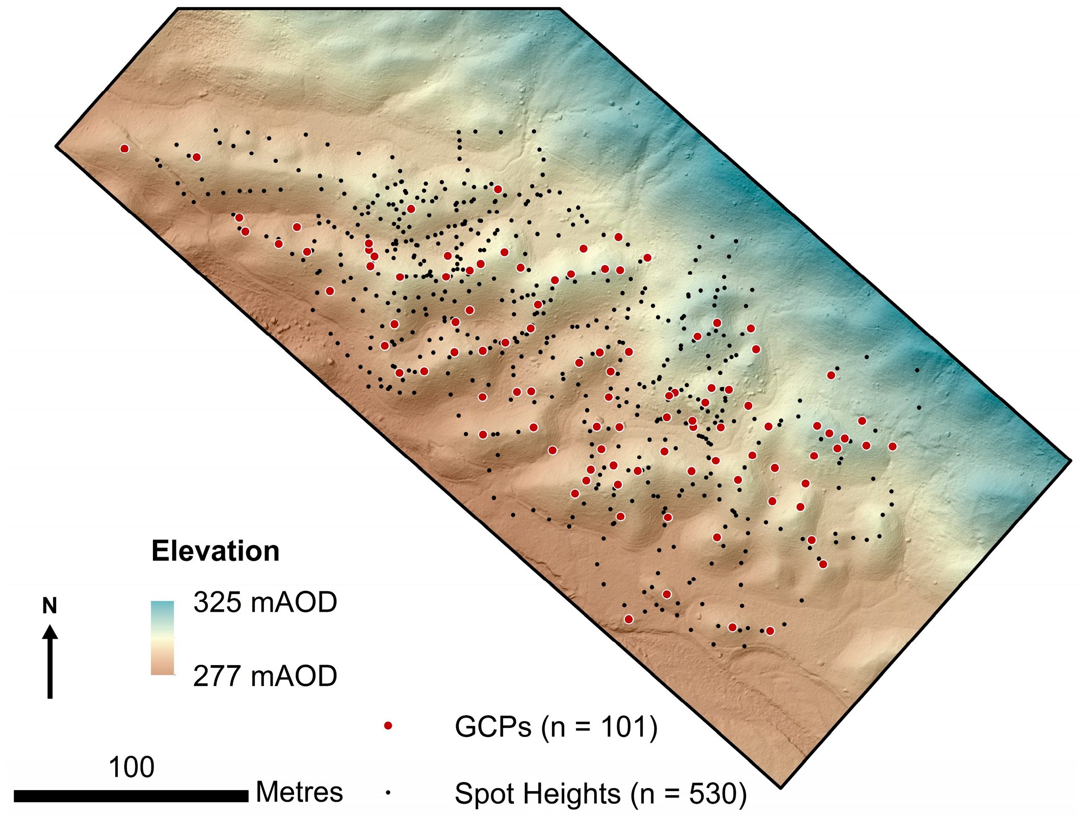
2. Field Site
3. Materials and Methods
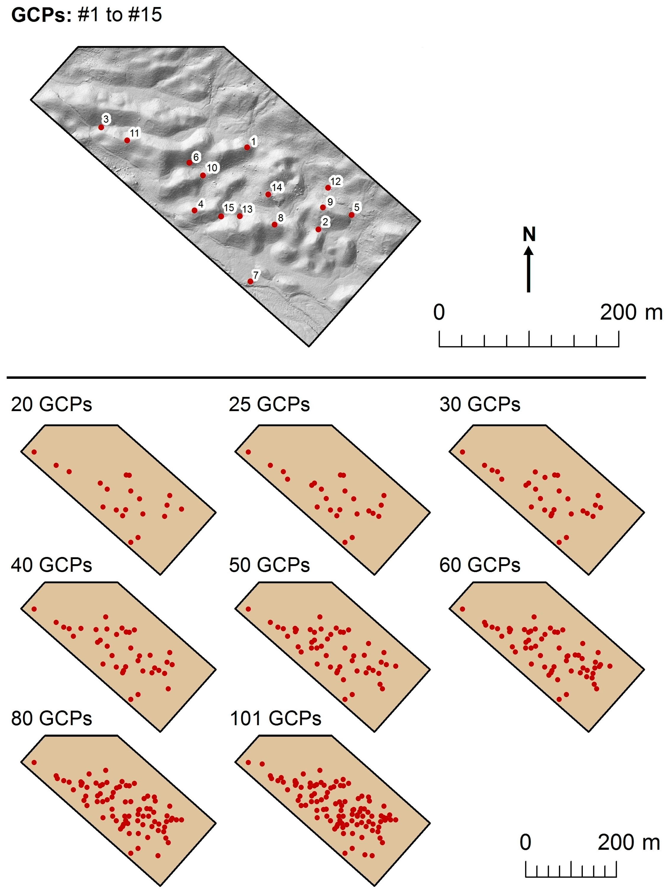
3.1. Data Acquisition
3.2. Data Analysis
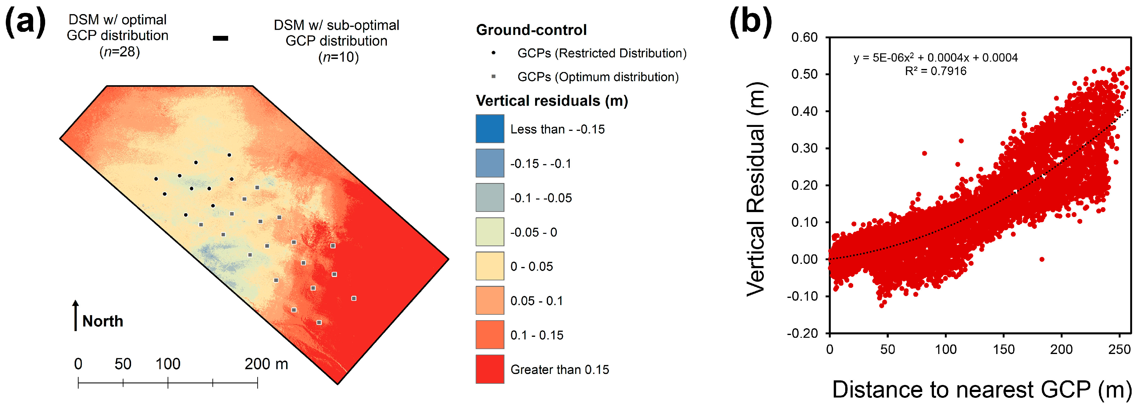
4. Results
5. Discussion
6. Conclusions
Acknowledgments
Author Contributions
Conflicts of Interest
References
- Anderson, K.; Gaston, K.J. Lightweight unmanned aerial vehicles will revolutionize spatial ecology. Front. Ecol. Environ. 2013, 11, 138–146. [Google Scholar] [CrossRef]
- Bemis, S.P.; Micklewaite, S.; Turner, D.; James, M.R.; Akciz, S.; Thiele, S.T.; Bangash, H.A. Ground-based and UAV-based photogrammetry: A multi-scale, high-resolution mapping tool for structural geology and paleoseismology. J. Struct. Geol. 2014, 69, 163–178. [Google Scholar] [CrossRef]
- Lucieer, A.; de Long, S.M.; Turner, D. Mapping landslide displacements using Structure from Motion (SfM) and image correlation of multi-temporal UAV photography. Prog. Phys. Geogr. 2014, 38, 97–116. [Google Scholar] [CrossRef]
- Lucieer, A.; Turner, D.; King, D.H.; Robinson, S.A. Using an Unmanned Aerial Vehicle (UAV) to capture micro-topography of Antarctic moss beds. Int. J. Appl. Earth Obs. Geoinf. 2014, 27, 53–62. [Google Scholar] [CrossRef]
- Woodget, A.; Carbonneau, P.; Visser, F.; Maddock, I. Quantifying submerged fluvial topography using hyperspatial resolution UAS imagery and structure from motion photogrammetry. Earth Surf. Proc. Landf. 2014, 40, 47–64. [Google Scholar] [CrossRef]
- Bhardwaj, A.; Sam, L.; Akanksha; Martín-Torresa, F.J.; Kumar, R. UAVs as remote sensing platform in glaciology: Present applications and future prospects. Remote Sens. Environ. 2016, 175, 196–204. [Google Scholar] [CrossRef]
- Verhoeven, G. Taking computer vision aloft—Archaeological three-dimensional reconstructions from aerial photographs with Photoscan. Archaeol. Prospect. 2011, 18, 67–73. [Google Scholar] [CrossRef]
- Westoby, M.J.; Brasington, J.; Glasser, N.F.; Hambrey, M.J.; Reynolds, J.M. ‘Structure-from-Motion’ photogrammetry: A low-cost, effective tool for geoscience applications. Geomorphology 2012, 179, 300–314. [Google Scholar] [CrossRef] [Green Version]
- Javernick, L.; Brasington, J.; Caruso, B. Modeling the topography of shallow braided rivers using Structure-from-Motion photogrammetry. Geomorphology 2014, 213, 166–182. [Google Scholar] [CrossRef]
- Nolan, M.; Larsen, C.; Sturm, M. Mapping snow depth from manned aircraft on landscape scales at centimeter resolution using structure-from-motion photogrammetry. Cryosphere 2015, 9, 1445–1463. [Google Scholar] [CrossRef]
- James, M.R.; Robson, S. Straightforward reconstruction of 3D surfaces and topography with a camera: Accuracy and geoscience application. J. Geophys. Res. Earth Surf. 2012, 117. [Google Scholar] [CrossRef] [Green Version]
- Eltner, A.; Braumgart, P.; Maas, H.-G.; Faust, D. Multi-temporal UAV data for automatic measurement of rill and interrill erosion on loess soil. Earth Surf. Process. Landf. 2014, 40, 741–755. [Google Scholar] [CrossRef]
- Tonkin, T.N.; Midgley, N.G.; Cook, S.J.; Graham, D.J. Ice-cored moraine degradation mapped and quantified using an unmanned aerial vehicle: A case study from a polythermal glacier in Svalbard. Geomorphology 2016, 258, 1–10. [Google Scholar] [CrossRef] [Green Version]
- Ryan, J.C.; Hubbard, A.L.; Box, J.E.; Todd, J.; Christoffersen, P.; Carr, J.R.; Holt, T.O.; Snooke, N. UAV photogrammetry and structure from motion to assess calving dynamics at Store Glacier, a large outlet draining the Greenland ice sheet. Cryosphere 2015, 9, 1–11. [Google Scholar] [CrossRef]
- Long, N.; Millescamps, B.; Guillot, B.; Pouget, F.; Bertin, X. Monitoring the topography of a dynamic tidal inlet using UAV imagery. Remote Sens. 2016, 8, 387. [Google Scholar] [CrossRef] [Green Version]
- Fonstad, M.A.; Dietrich, J.T.; Courville, B.C.; Jensen, J.L.; Carbonneau, P.E. Topographic structure from motion: A new development in photogrammetric measurement. Earth Surf. Process. Landf. 2013, 38, 421–430. [Google Scholar] [CrossRef]
- Tonkin, T.N.; Midgley, N.G.; Graham, D.J.; Labadz, J.C. The potential of small unmanned aircraft systems and structure-from-motion for topographic surveys: A test of emerging integrated approaches at Cwm Idwal, North Wales. Geomorphology 2014, 226, 35–43. [Google Scholar] [CrossRef] [Green Version]
- Clapuyt, F.; Veerle, V.; Van Oost, K. Reproducibility of UAV-based earth topography reconstructions based on Structure-from-Motion algorithms. Geomorphology 2016, 260, 4–15. [Google Scholar] [CrossRef]
- Jaud, M.; Passot, S.; Le Bivic, R.; Delacourt, C.; Grandjean, P.; Le Dantec, N. Assessing the accuracy of high resolution digital surface models computed by PhotoScan® and MicMac® in sub-optimal survey conditions. Remote Sens. 2016, 8, 465. [Google Scholar] [CrossRef]
- Smith, M.W.; Vericat, D. From experimental plots to experimental landscapes: Topography, erosion and deposition in sub-humid badlands from Structure-from-Motion photogrammetry. Earth Surf. Process. Landf. 2015, 40, 1656–1671. [Google Scholar] [CrossRef]
- Eltner, A.; Kaiser, A.; Castillo, C.; Rock, G.; Neugirg, F.; Abellán, A. Image-based surface reconstruction in geomorphometry–merits, limits and developments. Earth Surf. Dyn. 2016, 4, 359–389. [Google Scholar] [CrossRef]
- Smith, M.W.; Carrivick, J.L.; Quincey, D.J. Structure from motion photogrammetry in physical geography. Prog. Phys. Geogr. 2016, 40, 247–275. [Google Scholar] [CrossRef]
- Harwin, S.; Lucieer, A.; Osborn, J. The impact of the calibration method on the accuracy of point clouds derived using unmanned aerial vehicle multi-view stereopsis. Remote Sens. 2015, 7, 11933–11953. [Google Scholar] [CrossRef]
- Gómez-Gutiérrez, Á.; de Sanjosé-Blascom, J.J.; Lozano-Parra, J.; Berenguer-Sempere, F.; de Matías-Bejarano, J. Does HDR pre-processing improve the accuracy of 3D models obtained by means of two conventional SfM-MVS software packages? The case of the Corral del Veleta rock glacier. Remote Sens. 2015, 7, 10269–19294. [Google Scholar] [CrossRef]
- Sissons, J.B. The Loch Lomond Advance in the Lake District, northern England. Trans. R. Soc. Edinb. Earth Sci. 2015, 71, 13–27. [Google Scholar] [CrossRef]
- McDougall, D.A. The geomorphological impact of Loch Lomond (Younger Dryas) Stadial plateau icefields in the central Lake District, northwest England. J. Quat. Sci. 2001, 16, 531–543. [Google Scholar] [CrossRef]
- Graham, D.J.; Hambrey, M.J. Sediments and landforms in an upland glaciated-valley landsystem, upper Ennerdale, English Lake District. In Glacial Sedimentary Processes and Products; Hambrey, M.J., Christoffersen, P., Glasser, N.F., Hubbard, B., Eds.; International Association of Sedimentologists: Oxford, UK, 2007; pp. 235–256. [Google Scholar]
- Immerzeel, W.W.; Kraaijenbrink, P.D.A.; Shea, J.M.; Shrestha, A.B.; Pellicciotti, F.; Bierkens, M.F.P.; de Jong, S.M. High-resolution monitoring of Himalayan glacier dynamics using unmanned aerial vehicles. Remote Sens. Environ. 2015, 150, 93–103. [Google Scholar] [CrossRef]
- Carrivick, J.L.; Smith, M.W.; Quincey, D.J. Structure from Motion in the Geosciences; Wiley-Blackwell: Oxford, UK, 2016; p. 208. [Google Scholar]
- James, M.R.; Robson, S. Mitigating systematic error in topographic models derived from UAV and ground-based image networks. Earth Surf. Process. Landf. 2014, 39, 1413–1420. [Google Scholar] [CrossRef]


| Number of GCPs Used | Vertical RMSE (m) | Vertical MAE (m) | Vertical Difference (min; m) | Vertical Difference (max; m) |
|---|---|---|---|---|
| 3 | 0.156 | 0.126 | −0.462 | 0.427 |
| 4 | 0.064 | 0.049 | −0.206 | 0.291 |
| 5 | 0.060 | 0.046 | −0.197 | 0.308 |
| 7 | 0.062 | 0.048 | −0.175 | 0.353 |
| 8 | 0.073 | 0.058 | −0.192 | 0.257 |
| 9 | 0.063 | 0.049 | −0.173 | 0.283 |
| 10 | 0.075 | 0.059 | −0.195 | 0.400 |
| 15 | 0.076 | 0.061 | −0.179 | 0.270 |
| 20 | 0.073 | 0.057 | −0.190 | 0.280 |
| 25 | 0.073 | 0.057 | −0.178 | 0.352 |
| 30 | 0.067 | 0.052 | −0.177 | 0.269 |
| 40 | 0.066 | 0.050 | −0.191 | 0.304 |
| 50 | 0.060 | 0.046 | −0.143 | 0.282 |
| 60 | 0.064 | 0.047 | −0.160 | 0.548 |
| 80 | 0.061 | 0.047 | −0.156 | 0.242 |
| 101 | 0.059 | 0.045 | −0.147 | 0.277 |
© 2016 by the authors; licensee MDPI, Basel, Switzerland. This article is an open access article distributed under the terms and conditions of the Creative Commons Attribution (CC-BY) license (http://creativecommons.org/licenses/by/4.0/).
Share and Cite
Tonkin, T.N.; Midgley, N.G. Ground-Control Networks for Image Based Surface Reconstruction: An Investigation of Optimum Survey Designs Using UAV Derived Imagery and Structure-from-Motion Photogrammetry. Remote Sens. 2016, 8, 786. https://0-doi-org.brum.beds.ac.uk/10.3390/rs8090786
Tonkin TN, Midgley NG. Ground-Control Networks for Image Based Surface Reconstruction: An Investigation of Optimum Survey Designs Using UAV Derived Imagery and Structure-from-Motion Photogrammetry. Remote Sensing. 2016; 8(9):786. https://0-doi-org.brum.beds.ac.uk/10.3390/rs8090786
Chicago/Turabian StyleTonkin, Toby N., and Nicholas G. Midgley. 2016. "Ground-Control Networks for Image Based Surface Reconstruction: An Investigation of Optimum Survey Designs Using UAV Derived Imagery and Structure-from-Motion Photogrammetry" Remote Sensing 8, no. 9: 786. https://0-doi-org.brum.beds.ac.uk/10.3390/rs8090786