Article

Land Surface Temperature Differences within Local Climate Zones, Based on Two Central European Cities

1
Department of Geography, Faculty of Science, Masaryk University Brno, Kotlářská 2, 611 37 Brno, Czech Republic
2
Global Change Research Institute of the Czech Academy of Sciences, Bělidla 986/4a, 603 00 Brno, Czech Republic
3
Department of Geography, Faculty of Science, Palacký University Olomouc, 17. listopadu 12, 771 46 Olomouc, Czech Republic
*
Author to whom correspondence should be addressed.
Submission received: 20 June 2016 / Revised: 6 September 2016 / Accepted: 19 September 2016 / Published: 22 September 2016

Abstract

:
The main factors influencing the spatiotemporal variability of urban climate are quite widely recognized, including, for example, the thermal properties of materials used for surfaces and buildings, the mass, height and layout of the buildings themselves and patterns of land use. However, the roles played by particular factors vary from city to city with respect to differences in geographical location, overall size, number of inhabitants and more. In urban climatology, the concept of “local climate zones” (LCZs) has emerged over the past decade to address this heterogeneity. In this contribution, a new GIS-based method is used for LCZ delimitation in Prague and Brno, the two largest cities in the Czech Republic, while land surface temperatures (LSTs) derived from LANDSAT and ASTER satellite data are employed for exploring the extent to which LCZ classes discriminate with respect to LSTs. It has been suggested that correctly-delineated LCZs should demonstrate the features typical of LST variability, and thus, typical surface temperatures should differ significantly among most LCZs. Zones representing heavy industry (LCZ 10), dense low-rise buildings (LCZ 3) and compact mid-rise buildings (LCZ 2) were identified as the warmest in both cities, while bodies of water (LCZ G) and densely-forested areas (LCZ A) made up the coolest zones. ANOVA and subsequent multiple comparison tests demonstrated that significant temperature differences between the various LCZs prevail. The results of testing were similar for both study areas (89.3% and 91.7% significant LST differences for Brno and Prague, respectively). LSTs computed from LANDSAT differentiated better between LCZs, compared with ASTER. LCZ 8 (large low-rise buildings), LCZ 10 (heavy industry) and LCZ D (low plants) are well-differentiated zones in terms of their surface temperatures. In contrast, LCZ 2 (compact mid-rise), LCZ 4 (open high-rise) and LCZ 9 (sparsely built-up) are less distinguishable in both areas analyzed. Factors such as seasonality and thermal anisotropy remain a challenge for future research into LST differences.

Graphical Abstract

1. Introduction

The main factors influencing the spatiotemporal variability of urban climate are quite widely recognized, including, for example, the thermal properties of materials used for surfaces and buildings, the mass, height and layout of the buildings themselves and patterns of land use (e.g., [1,2]). However, urban climate research has long been limited by unsatisfactory quantification of these factors and non-standardized descriptions of them [3]. To address these problems in urban climatology, the concept of local climate zones (LCZs) has emerged over the past decade [4].
Stewart and Oke [4] define local climate zones as “regions of uniform land cover, surface structure, construction material and human activity that span hundreds of meters to several kilometers on a horizontal scale”. The thermal climate of each LCZ is determined by its surface character: structure (building and tree height/density), cover (permeability), fabric (albedo, thermal admittance) and metabolism (waste heat from transportation and space heating/cooling). Unique combinations of these properties provide a distinctive thermal regime for each LCZ, particularly the characteristic temperature regime at screen height, best observed in clear weather conditions and areas of simple relief [4,5].
The concept of the LCZ emerged out of the need to improve the documentation of atmospheric heat island observations, but its relation to spatial and temporal temperature variability has recently become a key research question [4,6,7]. Most recent studies investigating urban temperature fields utilize the LCZ classification and largely support the correspondence of LCZs with air temperature fields in cities and their surroundings (e.g., [6,8,9,10]). However, a number of authors working with LCZs have pointed out that the influence of thermal, radiative, metabolic and surface-cover properties on the formation of local climate may significantly vary with respect to the geographical location of the zone, the size of the city, the position within the city (distance from the city center, neighboring zones) and relief [11,12,13]. Simultaneously, Bechtel and Daneke [14] and Lelovics et al. [9] created the first LCZ mapping methods and applied the LCZ concept to secondary uses. With such an extension of LCZ beyond its primary function, certain new methodological problems appeared: the size of a spatial mapping unit, the method used for generalization, the temporal variability of the physical properties of the environment, the objectification and standardization of the classification procedure, and others [8,9,14]. The extension of LCZ to regional mapping significantly widens the field of LCZ applications. For instance, Alexander et al. [15] revealed distinctive heat fluxes for some LCZs and concluded that LCZ classification provides a useful sampling framework for the derivation of the land-cover fractions needed to run surface-energy balance models. Zuvela-Aloise et al. [16] and Geletič et al. [17] used LCZs as input to MUKLIMO_3, a non-hydrostatic micro-scale air temperature model. Further, Skarbit et al. [18,19] worked on the relations between LCZ and LST. The authors show that the different LCZ classes have different surface temperature characteristics as for their typical values and their frequency distribution. The latter will be addressed in this study in more detail because the statistical significance of the differences between the typical LST of climate zones will be analyzed.
From the nature of LCZ classification, standard or special-purpose near-surface air temperature measurements may be best suited to analyzing temperature contrasts among LCZs [6]. However, such measurements, even supplemented by measurements from a dense network of automatic stations, often prove insufficient to describe and understand fully the spatial variability of air temperature in urban areas [17,20]. These measurements are insufficient especially in terms of their ability to characterize temperature spatial distribution in detail, as the result may be dependent on the number of “point” measurements, the method of interpolation and more. Thus LSTs derived from various airborne or satellite remote sensing systems may be a suitable alternative, as their spatial coverage is complete. Moreover, spatial and temporal resolution is constantly improving [21,22,23]. In spite of the fact that surface temperature modulates the air temperature of the boundary layer atmosphere [21], relationships between the two types of temperature are quite complicated in urban environments [24,25,26]. Apparent urban LSTs are modified by numerous static (e.g., land cover type, urban morphology) and dynamic (e.g., geometry of thermal imagery acquisition, solar elevation) factors. These factors not only modify the energy balance of urban areas [1,4], but they also generate effects, such as thermal anisotropy [27]. Nevertheless, the use of land surface temperature for the analysis of temperature spatial variability and the estimation of urban heat island intensity remains challenging.
From all of this, it becomes clear that the LST characteristics typical of LCZs (if such definitive factors indeed exist) should be characterized in more detail in order to understand the influence of local climate zones on local climate formation better. Case studies using remote sensing data to investigate land surface temperatures (LSTs) from various cities may therefore contribute significantly to the study of LCZs. The particular aim of this study is to analyze relations between surface temperatures and local climate zones, taking two cities in the Czech Republic as examples. A new GIS-based method is used for LCZ delimitation. Compared to the widely-used method of Bechtel and Daneke [14], this method does not use thermal imagery, which is an important aspect as the paper explores the extent to which LCZ classes are delineated with respect to land surface temperatures.

2. Materials and Methods
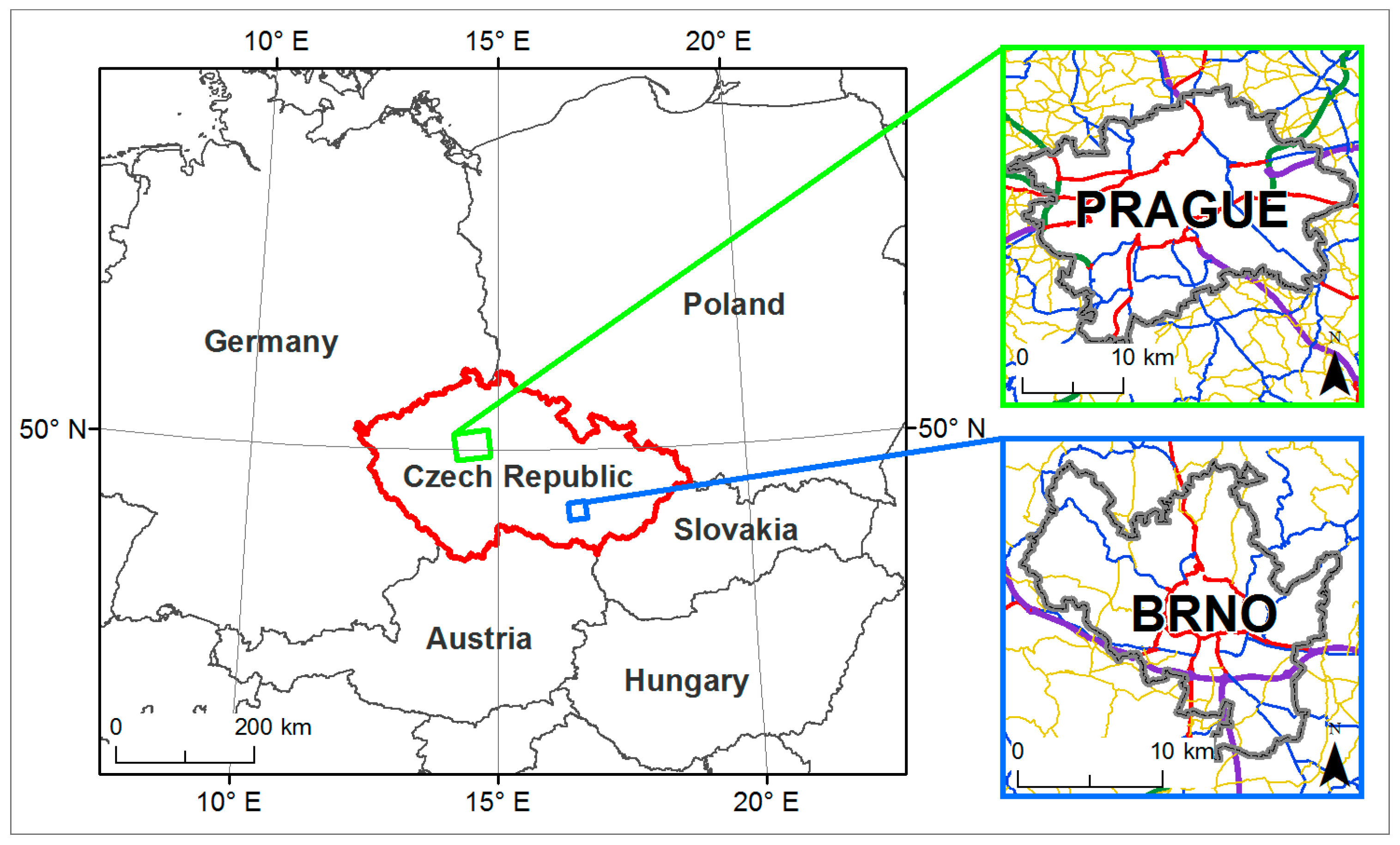
2.1. Study Area

This study focuses on Prague and Brno, the two largest cities in the Czech Republic. The capital Prague, with around 1.3 million inhabitants, as well as Brno, with fewer than 0.4 million inhabitants, may be considered as medium-sized cities typical of the central European region (Figure 1, Table 1).
In terms of urban morphology and relief, the cities are quite similar. Brno and Prague are both located in hilly landscapes. Altitudes vary from under 200 m to over 500 m in Brno and under 200 m to 400 m in Prague (mean elevations are 259 m for Brno and 288 m for Prague). Both cities have grown in concentric zones, reflecting the historical stages of their development. Building patterns show this clearly, and neither city lost significant proportions of their architectural heritage to the Second World War (clearly-defined historical center, residential buildings old and new, industrial areas, housing estates, modern shopping centers, malls and allotments). Because of this, neighborhoods with irregular, as well as regular (grid and radial grid) street plans are present in both cities. Differences between the cities are especially the presence of a large river (the Vltava) in Prague and a higher proportion of open vegetated (low plant) spaces in Brno. The landscapes beyond the city’s boundaries are of a predominantly agricultural character, with agricultural areas represented by low plants (cultivated plants like maize, barley, wheat or rapeseed; growing period beginning in April and harvest in August; fields not irrigated). Patches of orchards (LCZ B) and mixed forests (LCZ A) complete the landscape mosaics of the hinterlands (Brno also has large forested areas north of the city).
Mean annual temperature stands at 9.1 °C for Brno and 8.4 °C for Prague (1961–2000 reference period). The annual temperature regime is characterized by a single maximum (the warmest month being July with mean temperatures of 19.3 °C in Brno and 18.2 °C in Prague), with a single minimum (the coldest month is January with a mean temperature −1.9 °C in Brno and −1.4 °C in Prague). Mean annual precipitation totals are quite similar in both (505 mm for Brno and 526 mm for Prague) [28,29].

2.2. Local Climate Zones

A GIS-based approach was taken for the delimitation of LCZs [30]. This method had already been developed and tested in the area of Brno and its surroundings. It is based on the measurable physical properties of the environment and a clearly-defined decision-making algorithm. The algorithm derives from the basic physical parameters defined by Stewart and Oke [4]: building surface fraction (BSF), pervious surface fraction (PSF), impervious surface fraction (ISF) and height of roughness elements (HRE). These were supplemented by number of buildings (NoB). For the classification process, the study area was divided into a regular grid with cells of 100 m × 100 m, each cell exhibiting these physical parameters.
In the first step, cells were divided by BSF into two basic classes: building types and natural land cover types. In the second step, the cells in the first step categorized as building types (BSF ≥ 10%) were classified into particular LCZs on the basis of the smallest deviation from the optimum interval, as defined by Geletič and Lehnert [30] (against the background of values suggested by Stewart and Oke [4]; see Table 2) in terms of physical parameters (BSF, PSF, ISF and HRE). Industrial zones (LCZs 8 and 10) were refined using NoB. Cells that had been categorized as land-cover types in the first step were automatically classified into particular LCZs in the second step by means of the vector land use geodatabase [30].
When all cells had been assigned to an appropriate LCZ, the LCZ areas were delineated using a majority filter to smooth the results of classification. Independent testing of the decision-making algorithm for defining the percentage coverage for individual LCZs demonstrated close agreement with areas defined on the basis of expert knowledge (e.g., there was 90% agreement for Brno, not shown here). New LCZ maps for Brno and Prague were created for this particular study.

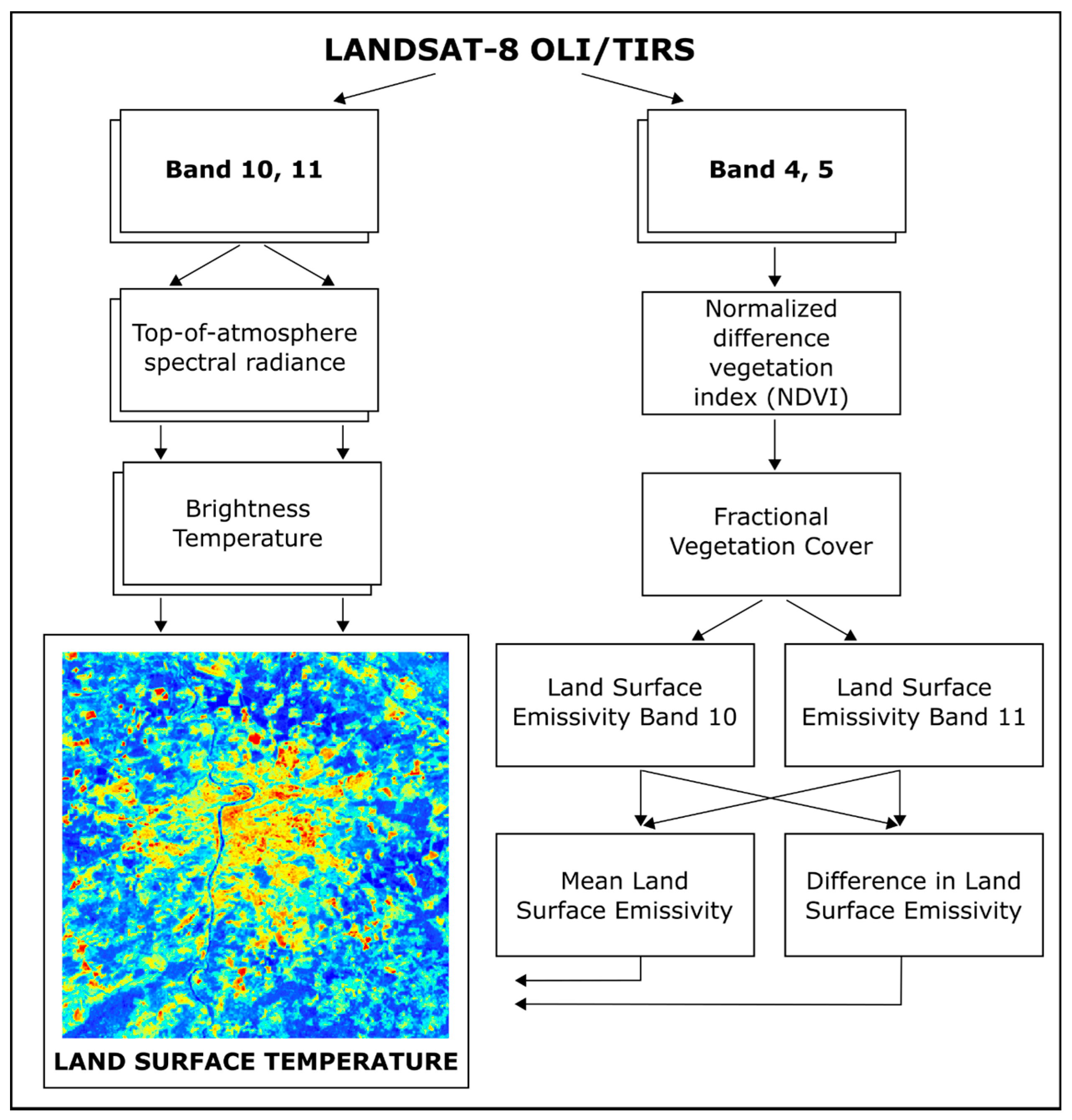
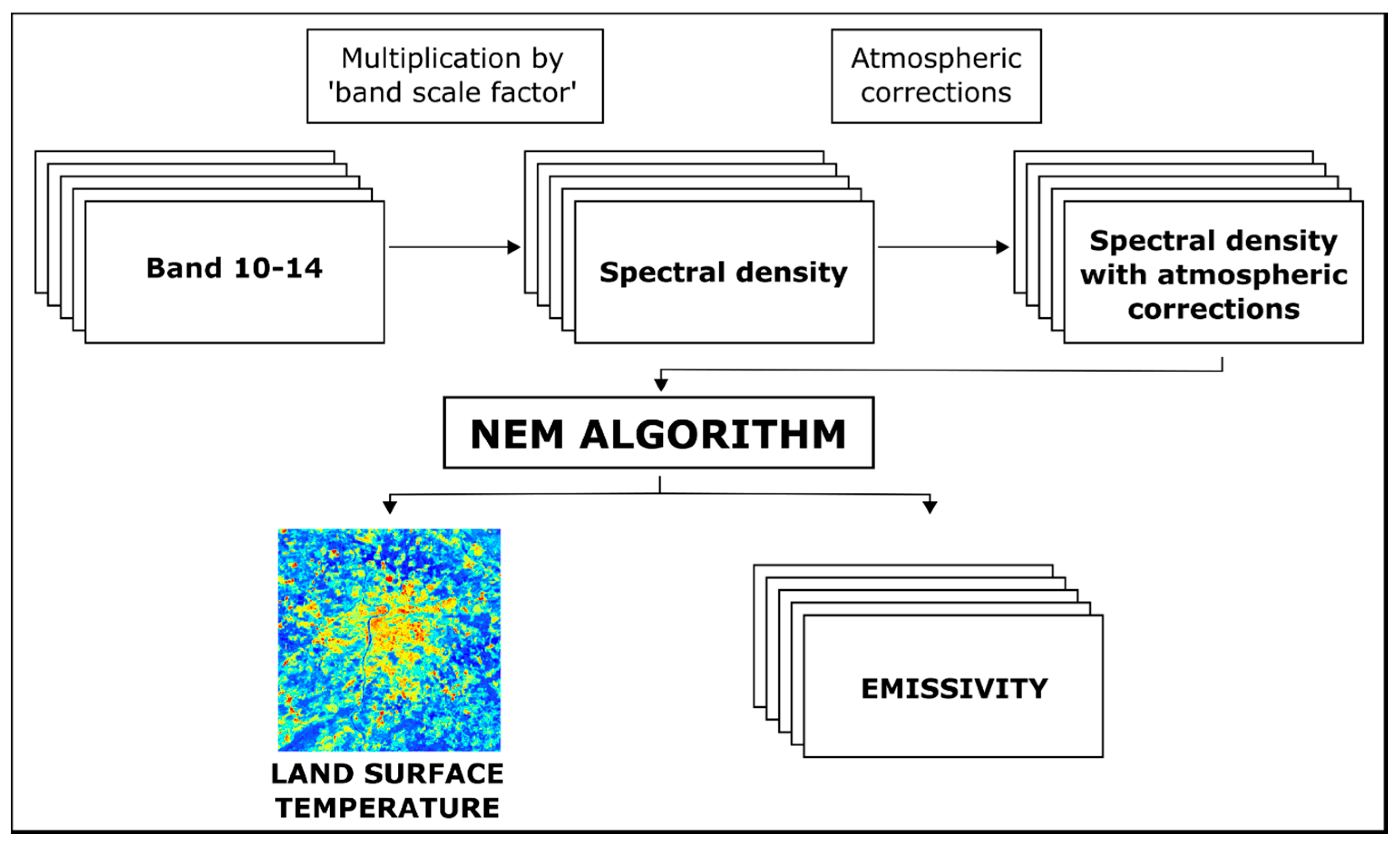
2.3. Land Surface Temperature

Land surface temperature (LST) was obtained from two satellites: LANDSAT-8 and Terra, sensor ASTER. LANDSAT-8 carries two instruments: an operational land imager (OLI) sensor and a thermal infrared sensor (TIRS). The OLI sensor has nine bands (Bands 1–7 and 9 at 30-m resolution, panchromatic Band 8 at 15-m resolution), while TIRS has two bands (Bands 10 and 11, collected at 100-m resolution and re-sampled to 30 m). ASTER consists of three separate instrument subsystems: visible near-infrared (VNIR; Bands 1–3, 15-m resolution), short-wave infrared (SWIR; Bands 4–9, at 30-m resolution) and thermal infrared (TIR; Bands 10–14, at 90-m resolution).
Altogether, 16 thermal images, eight for each city, four from LANDSAT-8 and four from ASTER, were used for the comparison with LCZs. Basic scene information is summarized in Table 3. For the interpretation of further analyses carried out in this study, it is important to emphasize that all thermal images were recorded in the morning daylight hours (except 19 July).
Two algorithms were used for the estimation of LST: split-window and multispectral. The split-window technique uses two thermal infrared (TIR) bands, typically located in the atmospheric window between 10 μm and 12 μm [31]. In this study, the algorithm applied was based on the estimation of top-of-atmosphere spectral radiance and at-satellite brightness temperature. LANDSAT-8 provides two thermal bands, Band 10 and Band 11 [32]. However, LANDSAT-8 does not provide data for surface emissivity calculation. Because of this, a land-surface emissivity (LSE) algorithm was used, estimating emissivity from the normalized difference vegetation index (NDVI) [33]. The scheme of LANDSAT-8 scene processing is summarized in Figure 2.
The thermal infrared bands on ASTER are located between 8 μm and 12 μm [34]. Two different approaches to the calculation of LST can be taken. The first exploits Level-1B data, which are produced by applying radiometric calibration and geometric correction coefficients. The multispectral algorithm for ASTER multiplies thermal bands by a scale factor, then atmospheric corrections are applied. The normalized emissivity (NEM) algorithm was used for LST calculation [34]. A schematic representation of this method appears in Figure 3. The ASTER product AST_08 (L2 surface kinetic temperature) may also be downloaded, but this option has only been available since 1 April 2016.

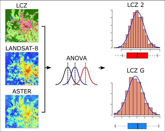
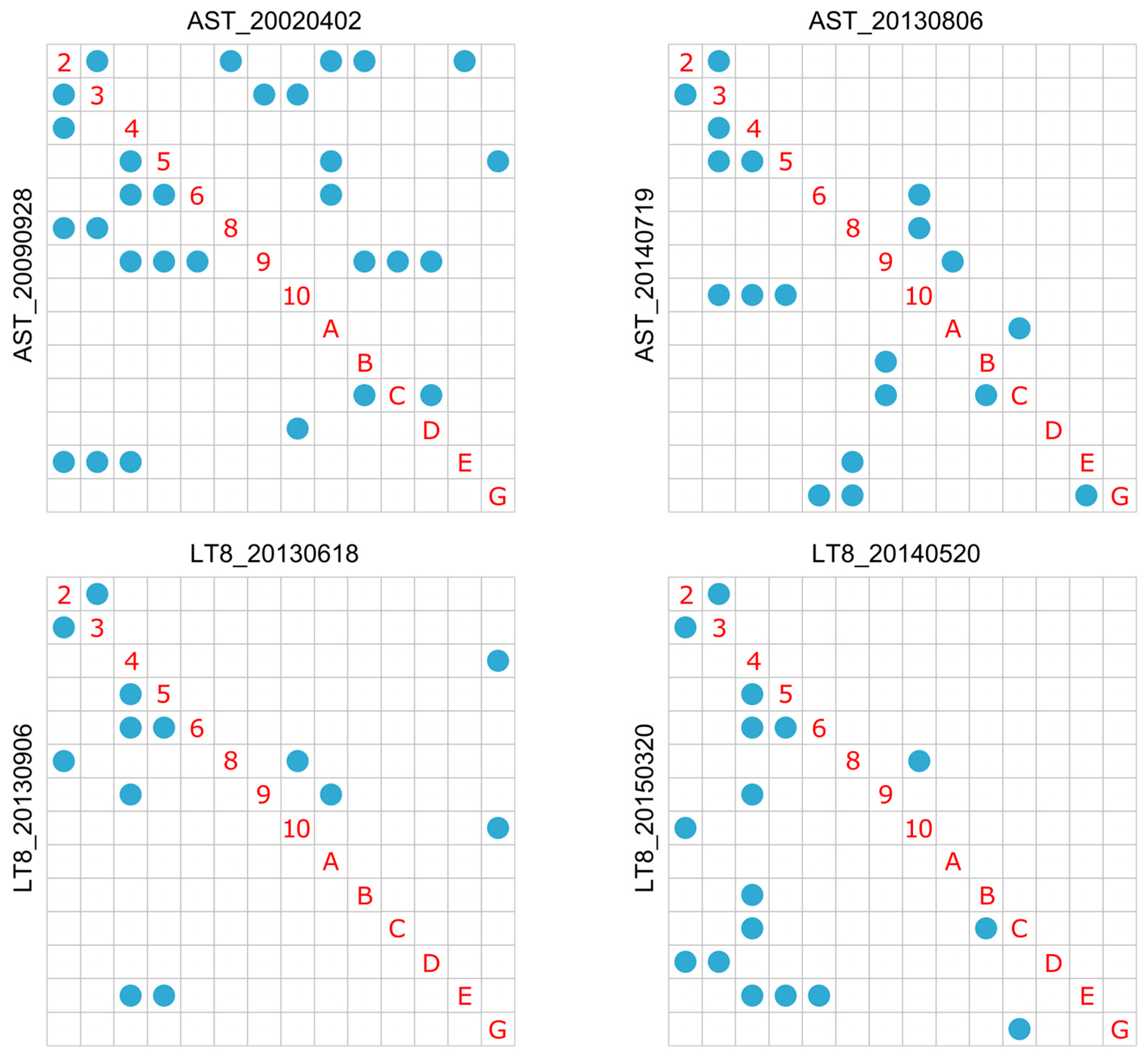
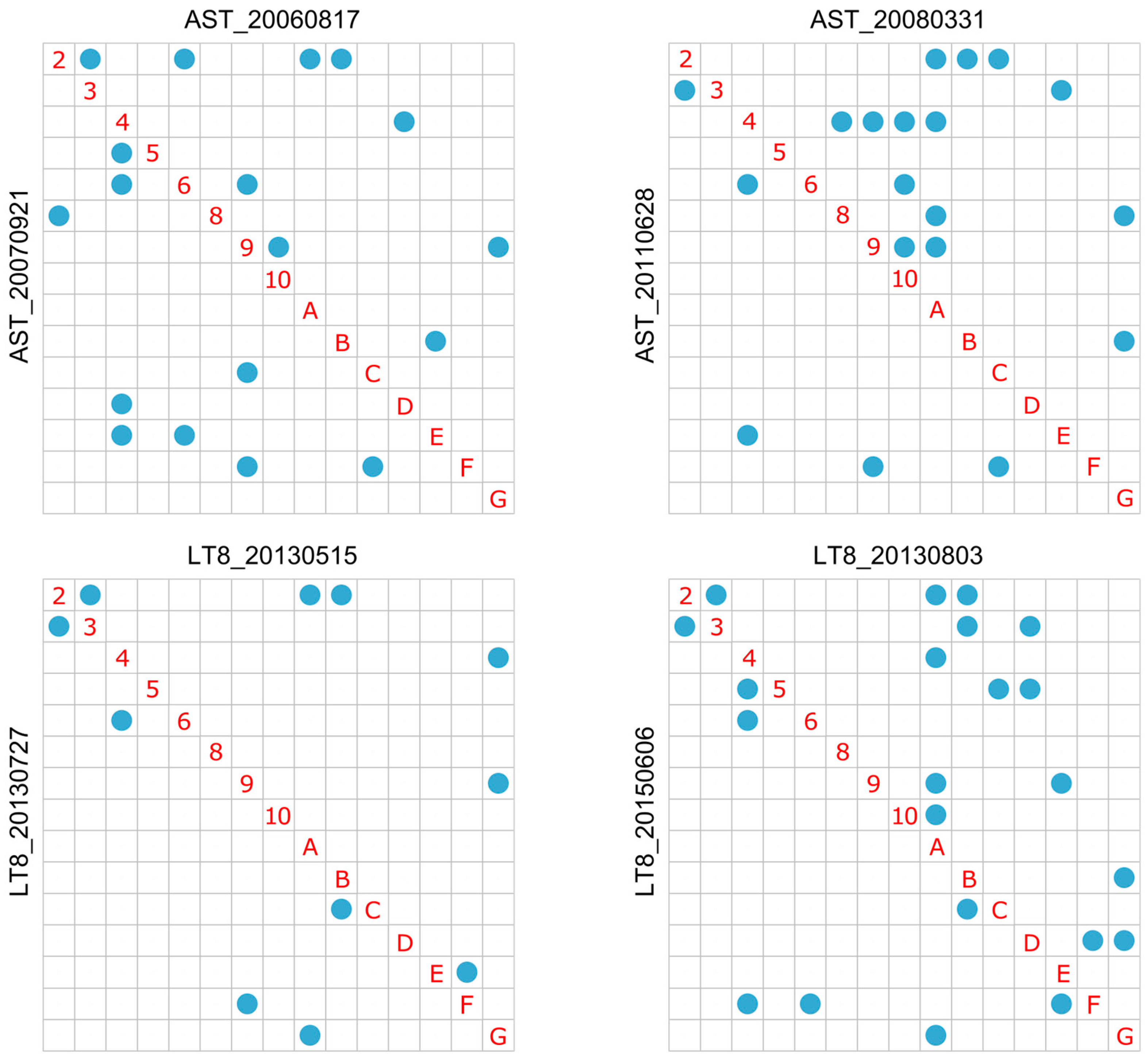
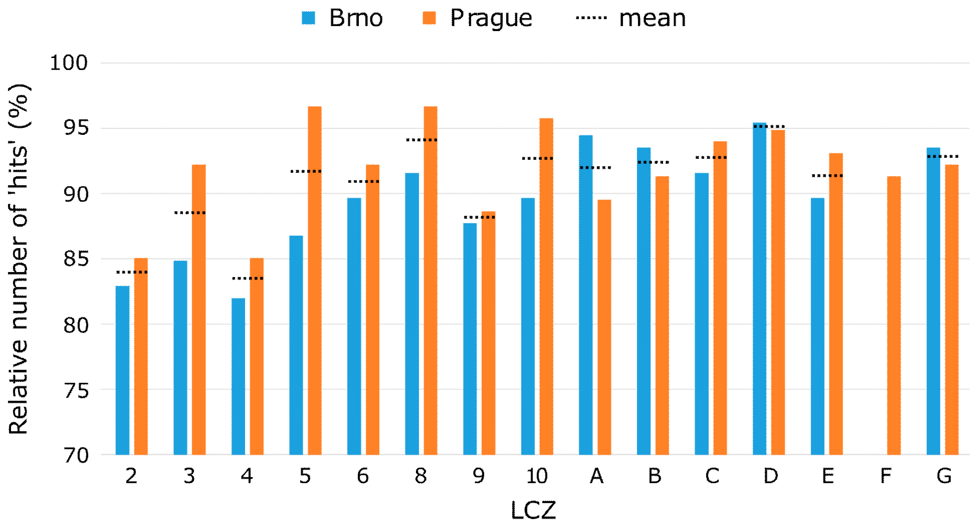
2.4. Comparison of Land-Surface Temperatures in Local Climate Zones
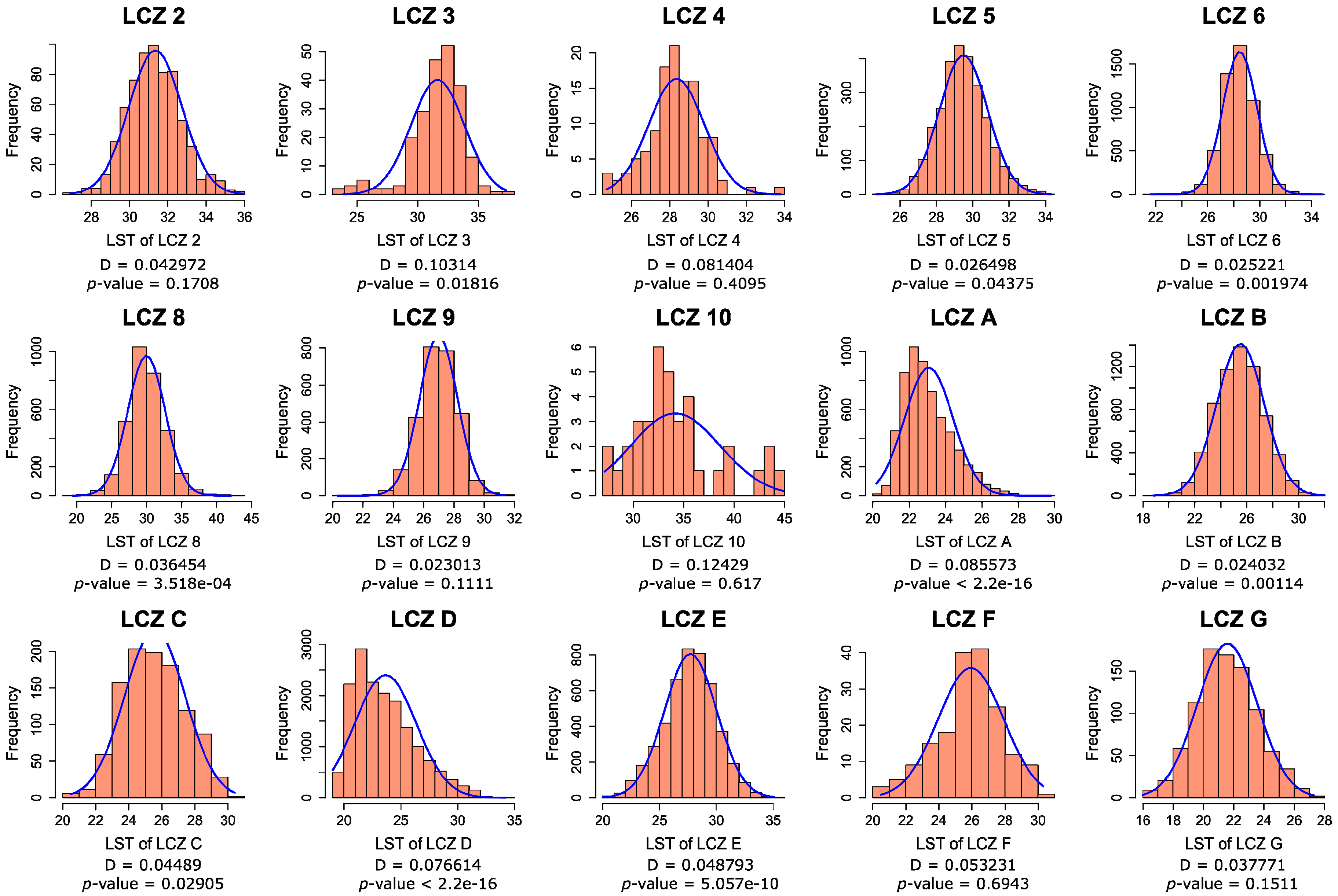
The analysis herein is based on the assumption that individual LCZs should demonstrate certain features typical of a given LST regime. LST fields were overlaid with LCZs, and typical LSTs were calculated for each zone. Differences between mean LCZ temperatures were evaluated by one-way analysis of variance (ANOVA). Before applying ANOVA, a careful assessment of assumptions for the application of this method was made. This comprised, in particular, testing for normality using the Kolmogorov–Smirnov tests, Q-Q plots and comparisons of LCZ temperature variability. When the ANOVA F-test indicated statistically-significant differences in LST, the Tukey HSD test was employed to control for the effect of multiple comparisons [35] and to reveal which LCZs differentiate significantly as to their mean LST. The analysis was performed separately for all 16 temperature fields constructed (two study areas with eight temperature fields each). Finally, the score counting the number of tests indicating significant temperature differences was calculated for each LCZ. Interpretation of this score is straightforward: LCZs with higher scores are better differentiated from other zones in terms of their typical LSTs. The other way round, LCZs with lower scores are less distinguishable from other zones in terms of their typical LSTs.

3. Results

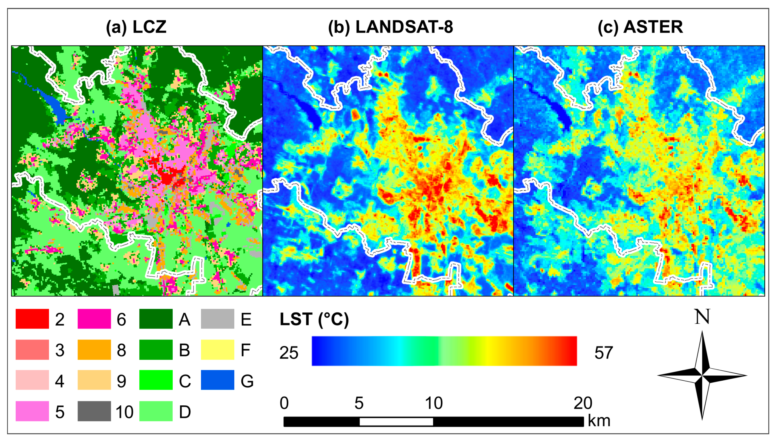
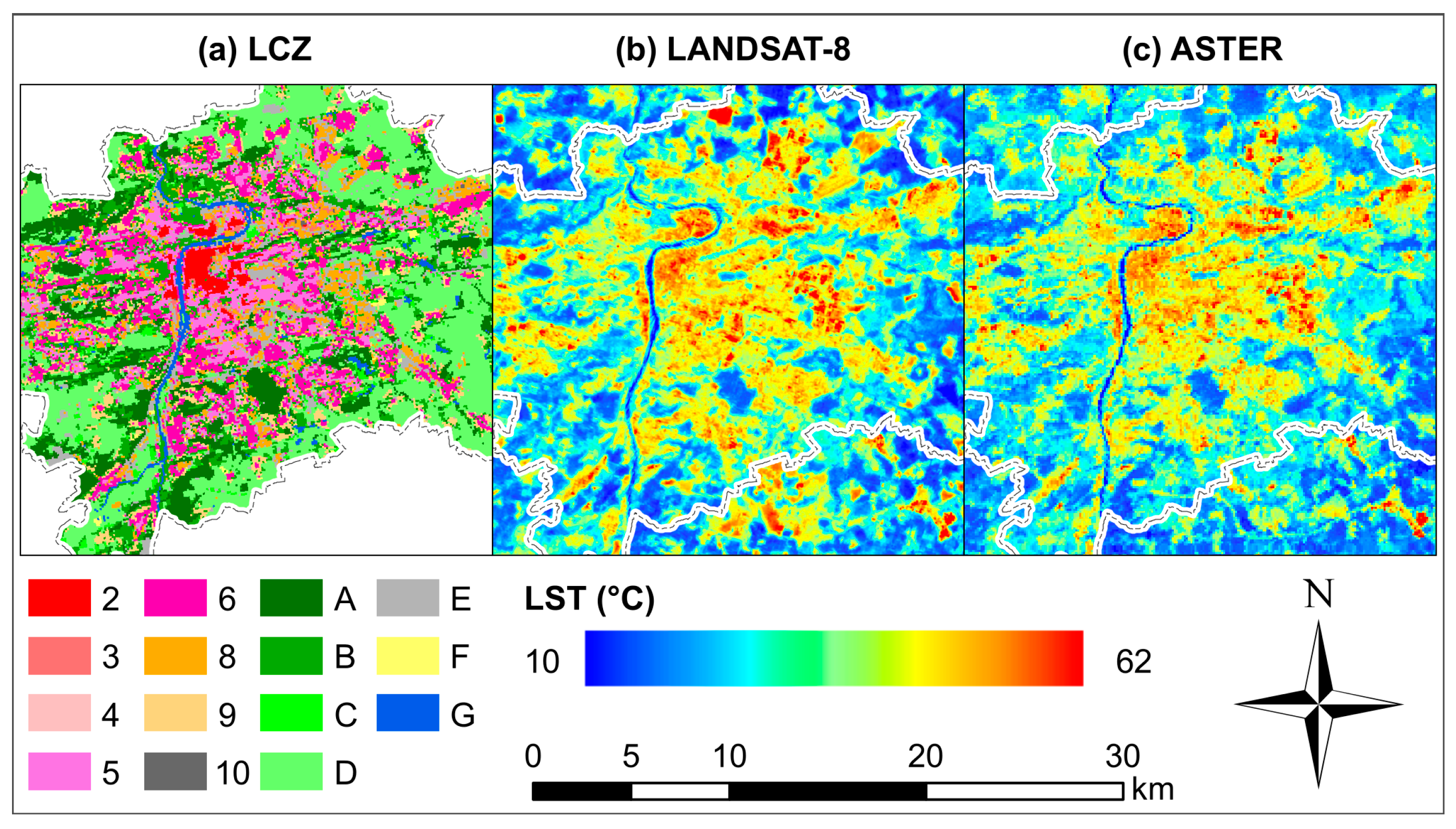
3.1. Local Climate Zones

The LCZ distributions exhibit concentric patterns, especially for Prague. The historical centers of Brno and Prague form compact areas of LCZ 2 (Figure 4 and Figure 5), clearly surrounded by LCZ 5, the most frequent type of development in both cities. Towards the outer boundaries of compact development, there is an increase in areas classified as LCZ 6. Together with LCZ 9, LCZ 6 is also typical of the villages around the cities. An increased occurrence of LCZ B is typical of the boundary between compact development and its surrounding landscape. LCZ B could, however, be found even near the centers of both cities (parks). LCZs 8, 10 and E appear especially on the outer part of the cities; these zones are frequently present in projections of development (city) into the surrounding countryside. Nevertheless, there are also the sites of LCZ 8, 10 and E in the core areas of both Brno (Figure 4) and Prague (Figure 5). LCZ D dominates in Prague’s surroundings, as it does in the landscape south of Brno, but to the north of Brno lie large areas of LCZ A. Also in the latter area is a large body of water, the Brno town reservoir, which creates a 259-ha area of LCZ G. Similarly, a line of LCZ G marks the course of the River Vltava in Prague.

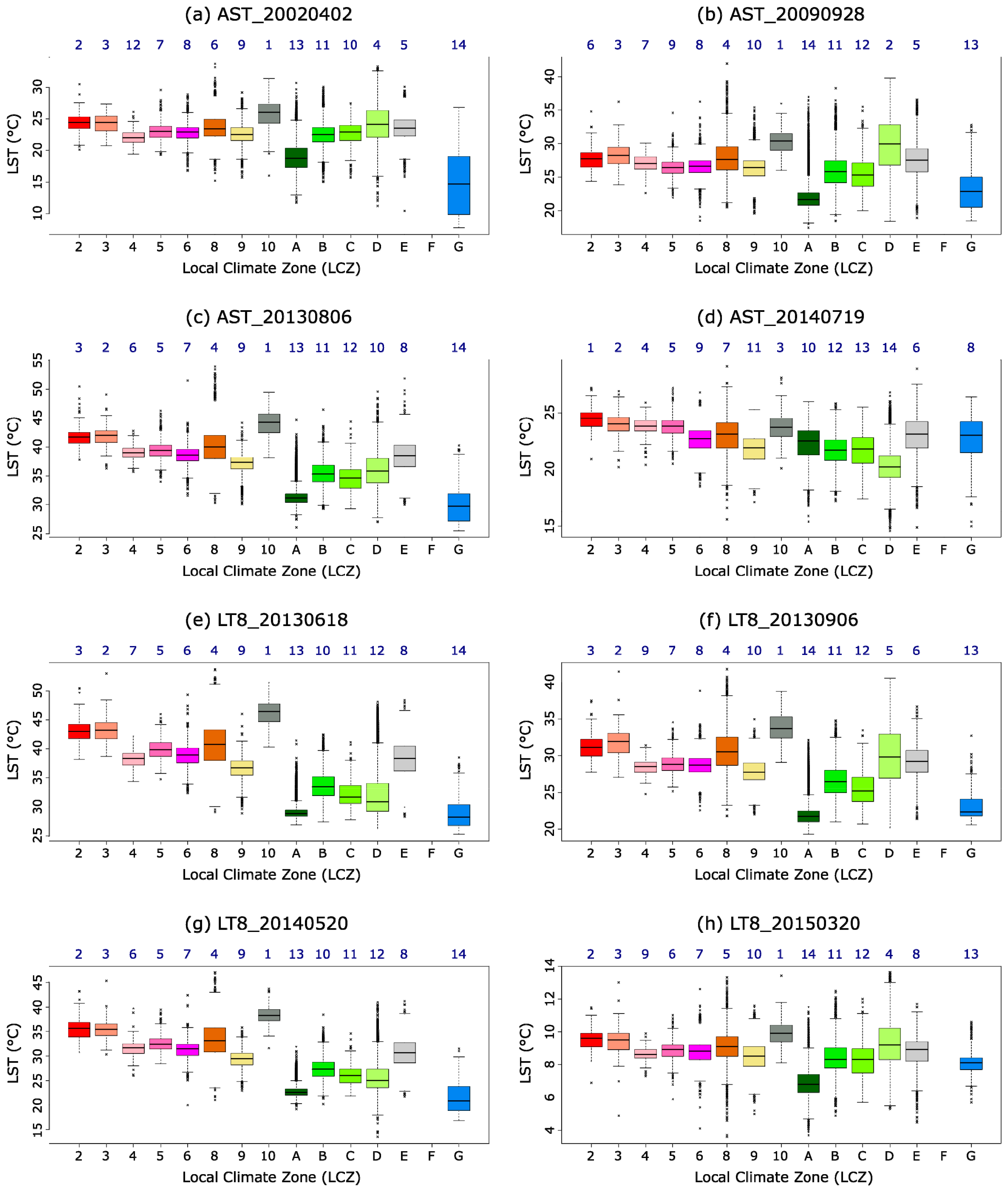
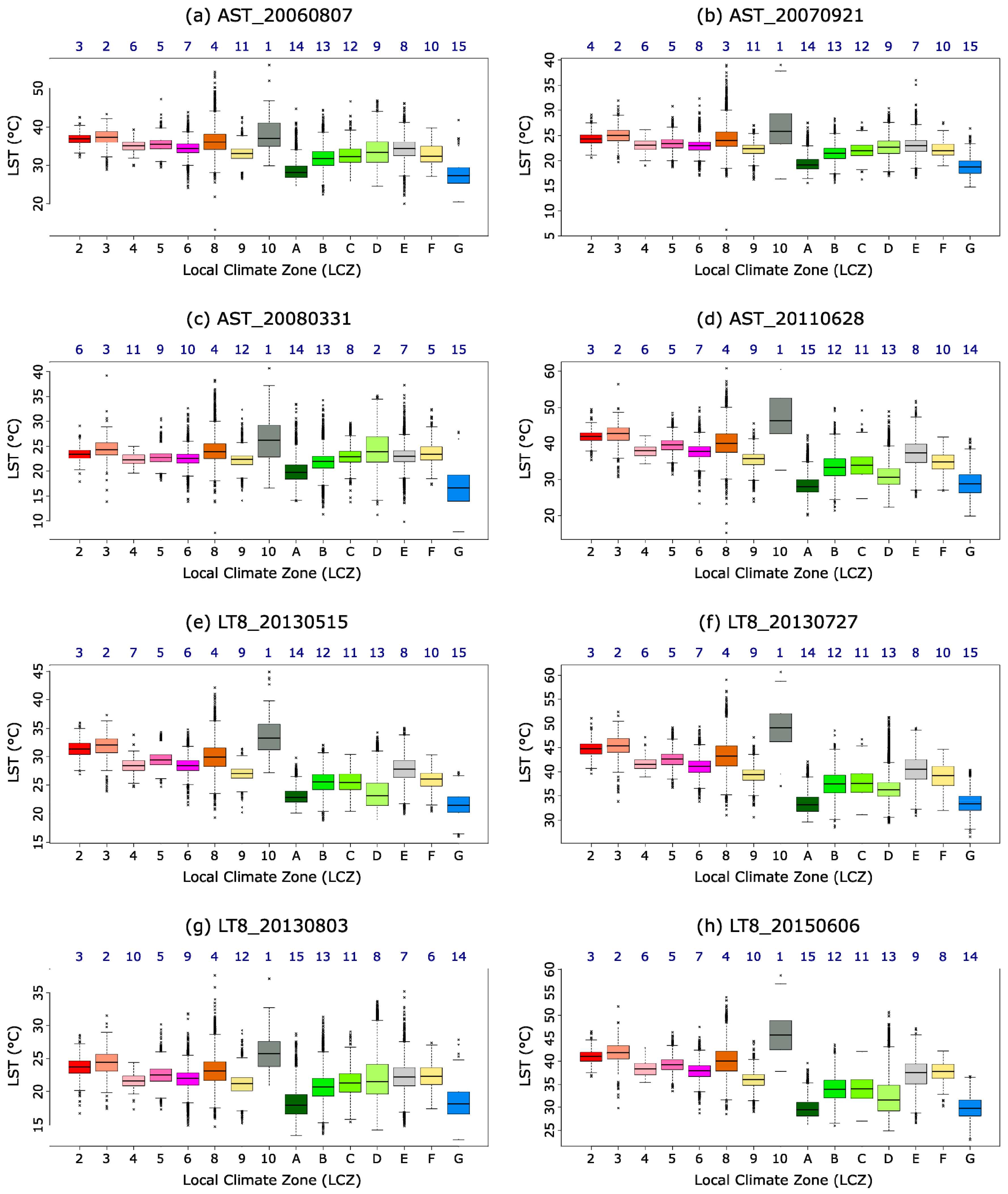
3.2. Land Surface Temperature

Brno and Prague show similar spatial distribution of surface temperatures. Industrial zones and the city centers with historical buildings were always warmer compared to their surroundings (Figure 4 and Figure 5). Away from the densely built-up areas, the warm parts of the cities also occurred near large patches of relatively flat, impervious surfaces (car parks, railway marshalling yards, stations, etc.). Hotspots were very often associated with large commercial and distribution areas and the international trade-fair grounds (which are quite extensive) regardless of whether they lay in the core of the city or in the countryside. On the other hand, bodies of water (the Brno reservoir and Prague’s River Vltava) and forested areas formed the coldest localities (see Figure 4 and Figure 5).

3.3. Local Climate Zones and Land Surface Temperatures

The spatial distributions of LCZs and LST presented above indicate that there is a certain degree of correspondence. Further analyses were therefore carried out to investigate their relations.
Box-plots summarizing typical LSTs for individual LCZs show relatively consistent results for the two cities (Figure 6 and Figure 7). However, the LSTs for LCZs derived from individual scenes cannot be further compared directly as they represent different days within a year, a period spanning 20 March–28 September (Table 3). Particular LSTs arose not only out of static factors (e.g., land cover), but were influenced by dynamic elements, such as the synoptic situation on a given day. Therefore, LSTs of LCZs were compared in terms of rank order within a set of eight analyzed scenes for each city. The mean LSTs of LCZs were sorted in descending order for each scene, and mean rankings were calculated from all scenes individually.
The majority highest mean LST emerged for LCZ 10 (heavy industry), which was the warmest for all eight scenes in Prague and for seven scenes in Brno. LCZ 3 (dense mix of low-rise buildings) and LCZ 2 (compact mid-rise buildings) were the second- and third-warmest zones in Brno and Prague. Next, higher LSTs were associated with LCZ 8 (large low-rise) in both study areas. The lowest ranking and, thus, the coolest LCZ was related to bodies of water (LCZ G) followed by LCZ A, areas with dense tree cover. Lower mean LSTs also occurred in other zones where pervious surfaces prevailed: LCZ B (scattered trees) and LCZ C (mixture of shrubs, woody trees and agricultural areas).
The box-plots in Figure 6 and Figure 7 present not only typical (median) LSTs for LCZs, but also permit the evaluation of their variability and the occurrence of outliers. Whereas LCZ temperature variations are more or less comparable and boxes and whiskers symmetrical, indicating no significant departures from normality, outliers typically occur in certain zones; they are analyzed further in the Discussion section below. The normality of the LST distribution in each LCZ was further tested more formally, since it is an important assumption for subsequent analysis of variance. A Gaussian curve was fitted to the LST frequency distribution for each zone and differences addressed by the Kolmogorov–Smirnov test. Figure 8 presents an example for a single date. Significant departures from normality occurred for several zones in Brno (LCZ 10 and G) and one in Prague (LCZ 10).
The results of the normality tests and comparable variations in LCZ land-surface temperatures indicated that ANOVA may be used for testing whether the differences in LCZ mean temperatures outlined above are significant or not.
Indeed, the results of the one-way ANOVA F-test (p < 0.001) determined that there exist significant differences among the means of LCZ land surface temperatures. Moreover, these results stand for the two study areas and for all 16 dates analyzed (scenes). Subsequently, Tukey HSD tests revealed which pairs of LCZs significantly differentiate in terms of their mean LSTs (Figure 9 and Figure 10).
Interpretation of all tests for both cities and analyzed scenes is provided in a simple binary format in Figure 9 and Figure 10. If the result of the test indicates no significant difference in average LSTs between two zones in question (p-value higher than 0.05), there is a blue point in the corresponding cell of the table. Blue points represent “negative” result in our analysis (“misses”), that is no difference in average LSTs for a given pair of LCZs. In contrast, if the result of the test shows significant difference (p-value lower than 0.05), there is an empty space in the corresponding cell of the table. Significant differences in average LSTs represent “positive” results in this analysis and may be denoted as “hits”.
Specifically, for both study areas, LCZ pairs with statistically-significant differences in mean LCZ temperatures (“hits”) prevail, while pairs with no temperature differences (“misses”) are less frequent, and such LCZ pairs are different in the individual scenes analyzed. This result strongly supports the method used for LCZ delimitation in both cities. That is, LCZs show typical surface temperatures that are largely quite different from the surface temperatures of other zones. The robustness of this finding is further confirmed by the fact that the relative number of “hits” is comparable for both cities (89.3% for Brno and 91.7% for Prague). Slightly larger differences may be found between the LSTs calculated from the two satellite data sources. Whereas ASTER-based LSTs indicate 89.2% hits, the LANDSAT-8-based LSTs show 91.9% hits. This implies that LSTs computed from LANDSAT-8 data better differentiate among various LCZs compared to those from ASTER.
A closer look at multiple comparison results facilitates the identification of zones that are well differentiated in terms of mean surface temperatures (Figure 11). The highest number of “hits” (significant temperature differences) was registered for LCZ 8 (large low-rise), LCZ 10 (heavy industry) and also for LCZ D (low plants). Such results confirm what is generally known of the spatial LST distribution in the areas analyzed. LCZs 8 and 10 consist of areas where impervious surfaces with lower proportions of vegetation cover prevail and where less surface moisture is available, features that are responsible for the higher surface temperatures of these zones. In both Czech cities, industrial areas are well delimited from neighborhoods that consist largely of LCZs with lower surface temperatures. In spite of the fact that LCZ D occurs in rural areas in which low plants prevail, typical land surface temperatures in this zone are markedly higher compared to their surroundings, due to the radiation response of soil (Figure 4 and Figure 5); see the Discussion section for details. LCZs with the lowest number of “hits” (those less distinguishable in terms of typical surface temperatures) may be identified in the same way. They stand for LCZ 2 (compact mid-rise), LCZ 4 (open high-rise) and LCZ 9 (sparsely built-up) in both areas analyzed. While LCZs 4 and 9 are characterized by somewhat lower LSTs, LCZ 2 represents zones with the highest mean surface temperatures; see Figure 6 and Figure 7 and the Discussion section below.

4. Discussion

This study is based on satellite (ASTER and LANDSAT-8) observations; therefore, bird’s eye-view surface temperatures from nadir (more precisely, nadir and very small off-nadir angles) are analyzed. The results here cannot therefore be equalized with respect to the general thermal responses of any particular LCZ, as vertical surfaces are neglected [20]; the results of this study thus provide a partial, but coherent, insight into the nature of surface temperatures in LCZs. Some noteworthy particularities and queries are addressed previously.
It was mentioned above that the highest LSTs were observed in LCZ 10 (heavy industry). However, when interpreting the thermal behavior of LCZ 10, it must be taken into account that LCZ 10 delineation was based on the Geletič and Lehnert [30] method, which employed a higher percentage of ISF and BSF for delineation of LCZ 10 than that originally suggested by Stewart and Oke [4]. Nevertheless, the higher land surface temperatures of industrial areas in daytime have previously been described by many authors, e.g., [28,36,37]. Unexpectedly, the LSTs of LCZ 8 (large low-rise) were in most cases considerably lower than the LSTs of LCZ 10. However, LCZ 8 was characterized by high statistical variability in LST. This may correspond to the different thermal properties implicit in the large roof surfaces that occur quite often in LCZ 8 [38]. LCZ A (dense trees) was identified as a lower LST zone, but a large number of positive outliers are evident (i.e., highest LST). This is a reaction to the relatively high number of patches, mostly consisting of clear-cuts of areas that are quite often below the spatial resolution of the data used for LCZ classification. On the other hand, the high LST variability of LCZ G (water) should be considered as realistic, since temperature differences reflect the different characters of individual bodies of water (depth, rate of flow, etc.). The LST of LCZ D also exhibited a relatively wide interquartile range with frequent outliers, especially for the upper part of the distribution. Considerable temperature differences between LCZ D and other zones are especially clearly expressed at the beginning and the end of the growing season, periods characterized by lower proportions of vegetation and the stronger radiation response of bare soil (lower albedo, reduced latent heat flux). This corresponds with the findings of [20,39,40] who described different spatial patterns of LST for spring and autumn compared to summer due to seasonal changes in land cover. Therefore, when working with LCZs, seasonal changes in land cover must be taken into consideration.
There were statistically-significant differences in mean LSTs between most LCZs, but LCZs 2, 4 and 9 were recognized as zones less distinguishable from other LCZs. A feature common to these three zones is the higher heterogeneity of land cover typical of central European cities. For instance, LCZ 2 might exhibit a range of building patterns (e.g., street canyons, courtyards) of various orientations to incoming solar radiation. This may significantly influence radiation response regarding both real surface temperature differences and the magnitude of effective anisotropy [14,27]. Moreover, the LSTs of LCZs 2 and 3 are similar because the percentages of PSF, ISF and BSF are also similar and the same types of materials for infrastructure, roofing, etc., are used (at least in central European conditions). One particular factor that differentiates these two zones is the height of the buildings; however, considering the nadir (or very close to nadir) view position of the sensors, the effect of vertical surfaces on apparent surface temperature is neglected, and simultaneously, dense development significantly reduces increase in shaded area (in the sense of direct solar radiation) with building height [41].
This analysis has indicated certain differences between the two sensor data sources (ASTER and LANDSAT-8). There may be several reasons for this. Each span leads to different LST retrieval algorithms to be used for LST calculation from ASTER and LANDSAT, arising out of the varying viewing geometry (IFOV (instantaneous field of view)) of the two satellite systems. In addition to this, land surface temperatures may be biased by several other factors arising from the nature of the remote sensing method. A higher proportion of vertically-oriented surfaces in urban areas compared to rural environments causes uneven solar heating of those surfaces and induces a thermal anisotropy effect [41]. Different solar heating of vertical surfaces arising out of variations in viewing geometry renders the interpretation of land surface temperatures problematic [27], and the effect of thermal anisotropy may influence the results of this study. According to Krayenhoff and Voogt [27], thermal anisotropy in an urban environment depends strongly on solar elevation and irradiance, and it increases in tall, closely-spaced buildings. Further, compact and high-rise zones generate greater anisotropy than open low-rise zones, while the regularity of street orientation increases anisotropy. As follows from the description of the study areas (see Section 2) and also from the results of LCZ mapping (Section 3), typical values of several of the above parameters should suffer less from the thermal anisotropy effect. Very high and closely-spaced buildings are quite rare in Prague and Brno. The average building height in the LCZ 2 zone of Prague is 19.9 m (typically between five and seven stories) and 20.9 m in Brno (typically 5–6 stories). Compact mid-rise zones (LCZ 2) constitute 1.32% and 0.31% of the Prague and Brno areas, respectively. Finally, streets are not regularly oriented in the two cities in the fashion typical of some larger cities elsewhere, e.g., in North America.
Moreover, one may assume that the negative effect of thermal anisotropy is partly suppressed in this study because eight different thermal images acquired from May–September were used. Different dates of data acquisition have slightly different viewing geometry and, thus, partly “average” the negative effect of thermal anisotropy. In spite of this, not only the bias due to thermal anisotropy, but also other aspects of LST (e.g., atmospheric corrections, LST~air temperature relationships) should be further clarified. However, these problems are beyond the scope of the current article.
It is important to stress that the same sets of warmest (coldest) LCZs were identified by both data sources. Last, but not least, an important precondition for LST comparison between different zones is mutual independence of LCZ classification and the surface temperature field. The GIS-based method used for LCZ delimitation in this study met this requirement. This is an important methodological aspect of this study with respect to widely-used imagery-based methods [14,42,43], including thermal bands for LCZ delimitation.

5. Conclusions

This paper compared the spatial distribution of land surface temperatures with local climate zones for the cities of Brno and Prague in the Czech Republic, employing data provided by two satellites. The cities studied are characterized by a similar spatial distribution of local climate zones previously constructed on the basis of a GIS method. This method utilizes data completely independent of those used for LST derivation, a feature that permitted the use of LSTs for unbiased investigation of the extent to which LCZs correspond with surface temperatures.
The key findings of this study may be summarized as follows: (i) regardless of the city studied or the satellite data employed, LSTs show typical surface temperatures that differ significantly between zones (in 89.3% and 91.7% of all tests applied for Brno and Prague, respectively); (ii) the warmest (LCZ 10, heavy industry; LCZ 3, dense low-rise buildings; LCZ 2, compact mid-rise buildings) and the coldest (LCZ G, water bodies; LCZ A, areas with dense trees) zones were identified in the two study areas; (iii) LCZ 8 (large low-rise), LCZ 10 (heavy industry) and LCZ D (low plants) were well differentiated in terms of surface temperatures; LCZ 2 (compact mid-rise), LCZ 4 (open high-rise) and LCZ 9 (sparsely built-up) constitute less clearly distinguishable zones in both cities.
It may be concluded that our findings generally support the concept of LCZs and the GIS-based method used for their delimitation for two typical central European cities of different sizes. Although the concept of LCZ was developed for the classification of air temperature measurements, the results of this paper confirm that individual LCZ prove also characteristic features of surface temperatures. Such conclusions were indicated in other studies [18,19,44]. In combination with the use of the GIS-based method, this LCZ-LST comparison may be considered the most important finding of this this contribution. Certain questions, such as seasonality in LST differences and thermal anisotropy (complete surface temperature differences), remain open to future research.

Acknowledgments

This contribution was prepared within the “UrbanAdapt—Development of urban adaptation strategies using ecosystem-based approaches to adaptation” project, supported by Grant EHP-CZ02-OV-1-036-2015 from Iceland, Liechtenstein and Norway and by the Ministry of Education, Youth and Sports of CZ within the National Sustainability Program I (NPU I), Grant Number LO1415. J.G. was also supported by the project MUNI/A/1315/2015. All ASTER images were retrieved from https://lpdaac.usgs.gov, maintained by the NASA EOSDIS Land Processes Distributed Active Archive Center (LP DAAC) at the USGS/Earth Resources Observation and Science (EROS) Center, Sioux Falls, South Dakota. The data product for the images was provided by NASA. The authors would like to thank the four anonymous reviewers who helped improve the manuscript. Tony Long (Svinošice) helped work up the English.

Author Contributions

J.G. performed the data analysis, prepared graphics and scripts and formatted the final manuscript. M.L. wrote the first draft and worked with J.G. on the paper. P.D. interpreted the analysis results and contributed to final text preparation. All authors contributed to the final manuscript and approved it.

Conflicts of Interest

The authors declare that there is no conflict of interest.

Abbreviations

The following abbreviations are used in this manuscript:
BSFBuilding Surface Fraction
ISFImpervious Surface Fraction
LCZLocal Climate Zones
LSTLand Surface Temperature
PSFPervious Surface Fraction

References

  1. Arnfield, A.J. Two decades of urban climate research: A review of turbulence, exchanges of energy and water, and the urban heat island. Int. J. Climatol. 2003, 23, 1–26. [Google Scholar] [CrossRef]
  2. Grimmond, C.B.S.; Ward, H.C.; Kotthaus, S. Effects of urbanization on local and regional climate. In The Routledge Handbook of Urbanization and Global Environmental Change, 1st ed.; Seto, K.C., Solecki, W.D., Griffith, C.A., Eds.; Routledge: London, UK; New York, NY, USA, 2016; pp. 169–187. [Google Scholar]
  3. Stewart, I.D. A systematic review and scientific critique of methodology in modern urban heat island literature. Int. J. Climatol. 2011, 31, 200–217. [Google Scholar] [CrossRef]
  4. Stewart, I.D.; Oke, T.R. Local climate zones for urban temperature studies. Bull. Am. Meteorol. Soc. 2012, 93, 1879–1900. [Google Scholar] [CrossRef]
  5. Stewart, I.D.; Oke, T.R. Local climate zones and urban climatic mapping. In The Urban Climatic Map: A Methodology for Sustainable Urban Planning, 1st ed.; Ren, C., Ng, E., Eds.; Routledge: New York, NY, USA, 2015; pp. 397–401. [Google Scholar]
  6. Stewart, I.D.; Oke, T.R.; Krayenhoff, E.S. Evaluation of the ‘local climate zone’ scheme using temperature observations and model simulations. Int. J. Climatol. 2014, 34, 1062–1080. [Google Scholar] [CrossRef]
  7. Gál, T.; Bechtel, B.; Unger, J. Comparison of two different local climate zone mapping methods. In Proceedings of the 9th International Conference on Urban Climate, Toulouse, France, 20–24 July 2015.
  8. Lehnert, M.; Geletič, J.; Husák, J.; Vysoudil, M. Urban field classification by “local climate zones” in a medium-sized Central European city: The case of Olomouc (Czech Republic). Theor. Appl. Climatol. 2015, 122, 531–541. [Google Scholar] [CrossRef]
  9. Lelovics, E.; Unger, J.; Gál, T.; Gál, V. Design of an urban monitoring network based on local climate zone mapping and temperature pattern modelling. Clim. Res. 2014, 60, 51–62. [Google Scholar] [CrossRef] [Green Version]
  10. Przybylak, R.; Uscka-Kowalkowska, J.; Araźny, A.; Kejna, M.; Kunz, M.; Maszewski, R. Spatial distribution of air temperature in Toruń (Central Poland) and its causes. Theor. Appl. Climatol. 2015. [Google Scholar] [CrossRef]
  11. Bokwa, A.; Hajto, M.J.; Walawender, J.P.; Szymanowski, M. Influence of diversified relief on the urban heat island in the city of Kraków, Poland. Theor. Appl. Climatol. 2015, 122, 365–382. [Google Scholar] [CrossRef]
  12. Leconte, F.; Bouyer, J.; Claverie, R.; Pétrissans, M. Using local climate zone scheme for UHI assessment: Evaluation of the method using mobile measurements. Build. Environ. 2015, 83, 39–49. [Google Scholar] [CrossRef]
  13. Lindén, J.; Grimmond, C.S.B.; Esper, J. Urban warming in villages. Adv. Sci. Res. 2015, 12, 157–162. [Google Scholar] [CrossRef]
  14. Bechtel, B.; Daneke, C. Classification of local climate zones based on multiple earth observation data. IEEE J. Sel. Top. Appl. Earth Obs. Remote Sens. 2012, 5, 1191–1202. [Google Scholar] [CrossRef]
  15. Alexander, P.J.; Mills, G.; Fealy, R. Using LCZ data to run an urban energy balance model. Urban Clim. 2015, 13, 14–37. [Google Scholar] [CrossRef]
  16. Zuvela-Aloise, M.; Bokwa, A.; Dobrovolný, P.; Gál, T.; Geletič, J.; Gulyas, Á.; Hajto, M.; Hollosi, B.; Kielar, R.; Lehnert, M.; et al. Modelling urban climate under global climate change in Central European cities. In Proceedings of the EGU General Assembly 2015, Vienna, Austria, 12–17 April 2015.
  17. Geletič, J.; Lehnert, M.; Dobrovolný, P. Modelled spatio-temporal variability of air temperature in an urban climate and its validation: A case study of Brno (Czech Republic). Hung. Geogr. Bull. 2016, 65, 169–180. [Google Scholar] [CrossRef]
  18. Skarbit, N.; Gal, T.; Unger, J. Airborne surface temperature differences of the different local climate zones in the urban area of a medium sized city. In Proceedings of the 2015 Joint Urban Remote Sensing Event (JURSE), Lausanne, Switzerland, 30 March–1 April 2015; pp. 1–4.
  19. Gémes, O.; Tobak, Z.; van Leeuwen, B. Satellite based analysis of surface urban heat island intensity. J. Environ. Geogr. 2016, 9, 23–30. [Google Scholar] [CrossRef]
  20. Dobrovolný, P.; Krahula, L. The spatial variability of air temperature and nocturnal urban heat island intensity in the city of Brno, Czech Republic. Morav. Geogr. Rep. 2015, 23, 8–16. [Google Scholar] [CrossRef]
  21. Voogt, J.A.; Oke, T.R. Thermal remote sensing of urban climates. Remote Sens. Environ. 2003, 86, 370–384. [Google Scholar] [CrossRef]
  22. Grimmond, C.B.S. Progress in measuring and observing the urban atmosphere. Theor. Appl. Climatol. 2006, 84, 3–22. [Google Scholar] [CrossRef]
  23. Weng, Q. Thermal infrared remote sensing for urban climate and environmental studies: Methods, applications, and trends. ISPRS J. Photogramm. 2009, 64, 335–344. [Google Scholar] [CrossRef]
  24. Gallo, K.P.; Owen, T.W. Satellite-based adjustments for the urban heat island temperature bias. J. Appl. Meteorol. 1999, 38, 806–813. [Google Scholar] [CrossRef]
  25. Unger, J.; Gál, T.; Rakonczai, J.; Mucsi, L.; Szatmári, J.; Tobak, Z.; van Leeuwen, B.; Fiala, K. Air temperature versus surface temperature in urban environment. In Proceedings of the 7th International Conference on Urban Climate, Yokohama, Japan, 29 June–3 July 2009.
  26. Schwarz, N.; Schlink, U.; Franck, U.; Großmann, K. Relationship of land surface and air temperatures and its implications for quantifying urban heat island indicators—An application for the city of Leipzig (Germany). Ecol. Indic. 2012, 18, 693–704. [Google Scholar] [CrossRef]
  27. Krayenhoff, E.S.; Voogt, J.A. Daytime thermal anisotropy of urban neighbourhoods: Morphological causation. Remote Sens. 2016, 8, 108. [Google Scholar] [CrossRef]
  28. Dobrovolný, P.; Řezníčková, L.; Brázdil, R.; Krahula, L.; Zahradníček, P.; Hradil, M.; Doleželová, M.; Šálek, M.; Štěpánek, P.; Rožnovský, J.; et al. Klima Brna. Víceúrovňová Analýza Městského Klimatu, 1st ed.; Masarykova Univerzita: Brno, Czech Republic, 2012. [Google Scholar]
  29. Tolasz, R.; Brázdil, R.; Bulíř, O.; Dobrovolný, P.; Dubrovský, M.; Hájková, L.; Halásová, O.; Hostýnek, J.; Janouch, M.; Kohut, M.; et al. Atlas Podnebí Česka: Climate Atlas of Czechia, 1st ed.; Praha, Olomouc: Český Hydrometeorologický Ústav, Czech Republic, 2007. [Google Scholar]
  30. Geletič, J.; Lehnert, M. A GIS-based delineation of local climate zones: The case of medium-sized Central European cities. Morav. Geogr. Rep. 2016, 24, 25–35. [Google Scholar]
  31. Sobrino, J.A.; Li, Z.L.; Stoll, M.P.; Becker, F. Multi-channel and multi-angle algorithms for estimating sea and land surface temperature with ATSR data. Int. J. Remote Sens. 1996, 17, 2089–2114. [Google Scholar] [CrossRef]
  32. U.S. Geological Survey, Department of the Interior. LANDSAT 8 (L8) Data Users Handbook (Version 2.0). 2016; U.S. Geological Survey LANDSAT Missions Web Site. Available online: https://landsat.usgs.gov/documents/Landsat8DataUsersHandbook.pdf (accessed on 30 May 2016). [Google Scholar]
  33. Rozenstein, O.; Qin, Z.; Derimian, Y.; Karnieli, A. Derivation of land surface temperature for Landsat-8 TIRS using a split window algorithm. Sensors 2014, 14, 5768–5780. [Google Scholar] [CrossRef] [PubMed]
  34. Gillespie, A.R.; Rokugawa, S.; Hook, S.J.; Matsunaga, T.; Kahle, A.B. Temperature/Emissivity Separation Algorithm Theoretical Basis Document (Version 2.4). 1999; NASA’s Earth Observing System Project Science Office Web Site. Available online: http://eospso.nasa.gov/sites/default/files/atbd/atbd-ast-05-08.pdf (accessed on 30 May 2016). [Google Scholar]
  35. Livezey, R.E. Field intercomparison. In Analysis of Climate Variability: Applications of Statistical Techniques, 2nd ed.; von Storch, H., Navarra, A., Eds.; Springer: New York, NY, USA; Heidelberg, Germany, 1995; pp. 161–178. [Google Scholar]
  36. Roth, M.; Oke, T.R.; Emery, W.J. Satellite-derived urban heat islands from three coastal cities and the utilization of such data in urban climatology. Int. J. Remote Sens. 1989, 10, 1699–1720. [Google Scholar] [CrossRef]
  37. Stathopoulou, M.; Cartalis, C.; Chrysoulakis, N. Using midday surface temperature to estimate cooling degree-days from NOAA-AVHRR thermal infrared data: An application for Athens, Greece. Sol. Energy 2006, 80, 414–422. [Google Scholar] [CrossRef]
  38. Akbari, H.; Levinson, R. Evolution of cool-roof standards in the US. Build. Energy Res. 2008, 1, 1–32. [Google Scholar] [CrossRef]
  39. Dobrovolný, P. The surface urban heat island in the city of Brno (Czech Republic) derived from land surface temperatures and selected reasons for its spatial variability. Theor. Appl. Climatol. 2013, 112, 89–98. [Google Scholar] [CrossRef]
  40. Wang, J.; Huang, B. Future urban climatic map development based on spatiotemporal image fusion for monitoring the seasonal response of urban heat islands to land use/cover. In The Urban Climatic Map: A Methodology for Sustainable Urban Planning, 1st ed.; Ng, E., Ren, C., Eds.; Routledge: New York, NY, USA, 2015; pp. 408–417. [Google Scholar]
  41. Voogt, J.A.; Oke, T.R. Effects of urban surface geometry on remotely-sensed surface temperature. Int. J. Remote Sens. 1998, 19, 895–920. [Google Scholar] [CrossRef]
  42. Bechtel, B.; Alexander, P.J.; Böhner, J.; Ching, J.; Conrad, O.; Feddema, J.; Mills, G.; See, L.; Stewart, I. Mapping local climate zones for a worldwide database of the form and function of cities. ISPRS Int. J. Geo-Inf. 2015, 4, 199–219. [Google Scholar] [CrossRef]
  43. Danylo, O.; See, L.; Bechtel, B.; Schepaschenko, D.; Fritz, S. Contributing to WUDAPT: A local climate zone classification of two cities in Ukraine. IEEE J. Sel. Top. Appl. Earth Obs. Remote Sens. 2015, 9, 1841–1853. [Google Scholar]
  44. Lin, Z.; Xu, H. A study of urban heat island intensity based on “local climate zones”: A case study in Fuzhou, China. In Proceedings of the 4th International Workshop on Earth Observation and Remote Sensing Applications (EORSA), Guangzhou, China, 4–6 July 2016.
Figure 1. Locations of Brno and Prague within central Europe and demarcation of the study areas with cadastral borders of compact urban development.
Remotesensing 08 00788 g001
Figure 2. LST calculation from LANDSAT-8 OLI/TIRS images.
Remotesensing 08 00788 g002
Figure 3. LST calculation from ASTER thermal images.
Remotesensing 08 00788 g003
Figure 4. (a) Spatial distribution of LCZs and examples of (b) LANDSAT-8, scene LT8_20150606, and (c) ASTER, scene AST_20110628; surface temperature variability in the Prague area; see Table 3 for the scene ID. LCZ key: 2, compact mid-rise; 3, compact low-rise; 4, open high-rise; 5, open mid-rise; 6, open low-rise; 8, large low-rise; 9, sparsely built-up; 10, heavy industry; A, dense trees; B, scattered trees; C, bush, scrub; D, low plants; E, bare rock or paved; F, bare soil or sand; G, water.
Remotesensing 08 00788 g004
Figure 5. (a) Spatial distribution of LCZs and examples of (b) LANDSAT-8, scene LT8_20130618, and (c) ASTER, scene AST_20130806; LST variability in the Brno area; see Table 3 for the scene ID. LCZ key: 2, compact mid-rise; 3, compact low-rise; 4, open high-rise; 5, open mid-rise; 6, open low-rise; 8, large low-rise; 9, sparsely built-up; 10, heavy industry; A, dense trees; B, scattered trees; C, bush, scrub; D, low plants; E, bare rock or paved; F, bare soil or sand; G, water.
Remotesensing 08 00788 g005
Figure 6. Box-plots with LSTs in LCZ classes in Brno for ASTER (ad) and LANDSAT-8 (eh) images; see Table 3 for the scene ID; the line within the box indicates median. The bottom of the box is the first quartile, and the top is the third quartile. Whiskers represent the lowest value still within 1.5 IQR (IQR = third quartile − first quartile) and the highest value still within 1.5 IQR. Black crosses indicate outliers. The top row with blue numbers indicates the order of LCZ according to the average LST (1, the warmest zone; 14, the coldest zone).
Remotesensing 08 00788 g006
Figure 7. Box-plots with land surface temperature (LST) in LCZ classes in Prague for ASTER (ad) and LANDSAT-8 (eh) images; see Table 3 for the scene ID; for the explanation, see Figure 6.
Remotesensing 08 00788 g007
Figure 8. Frequency distribution of land-surface temperatures in LCZ classes completed with a fitted normal distribution and with the results of the Kolmogorov–Smirnov test. D stands for the testing criterion, and p is the corresponding p-value. A p-value less than 0.05 indicates departure from normality. The example features Prague, LANDSAT-8, 6 June 2015.
Remotesensing 08 00788 g008
Figure 9. Results of the Tukey-HSD test for all combinations of LCZ classes (red numbers and letters) and for all analyzed scenes in Brno; see Table 3 for the scene ID; blue points indicate pairs of LCZs for which LSTs are not significantly different (p > 0.05), while empty cells denote LCZs pairs for which average LSTs are significantly different.
Remotesensing 08 00788 g009
Figure 10. Results of the Tukey-HSD test for all combinations of LCZ classes (red numbers and letters) and for all analyzed scenes in Prague; see Table 3 for the scene ID; blue points indicate pairs of LCZs for which land surface temperatures are not significantly different (p > 0.05), while empty cells denote LCZs pairs for which their average LSTs are significantly different.
Remotesensing 08 00788 g010
Figure 11. Relative number of multiple comparison tests indicating significant differences (p < 0.05) in LST (“hits”) among LCZs in Brno and Prague; LCZ F does not occur in Brno; dotted lines indicate mean values for the two cities.
Remotesensing 08 00788 g011
Table 1. Basic data, study areas.
LocationSize of Study AreaCadastral AreaNumber of InhabitantsMean ElevationLatitude (City Center)Longitude (City Center)
Brno and surroundings25 × 25 km8266 ha400,000259 m49°12′N16°37′E
Prague and surroundings35 × 25 km49,600 ha1,275,000288 m50°05′N14°25′E
Table 2. Selected surface cover properties of the local climate zones valid for the central European region ([4], modified); BSF, building surface fraction; ISF, impervious surface fraction; PSF, pervious surface fraction; HRE, height of roughness elements.
LCZTypeBSF (%)ISF (%)PSF (%)HRE (m)
1Compact high-rise40–6040–60<10>25
2Compact mid-rise40–7030–50<2010–25
3Compact low-rise40–7020–50<303–10
4Open high-rise20–4030–40(30–50) 30–40>25
5Open mid-rise20–4030–50(30–60) 20–4010–25
6Open low-rise20–4020–5030–603–10
7Lightweight low-rise60–90<20<302–4
8Large low-rise30–5040–50<203–10
9Sparsely built10–20<2060–803–10
10Heavy industry(40–70) 20–30(30–60) 20–40(<10) 40–50(10–20) 5–15
ADense trees<10<10>903–30
BScattered trees<10<10>903–15
CBush, scrub<10<10>90<2
DLow plants<10<10>90<1
EBare rock or paved<10>90<10<0.25
FBare soil or sand<10<10>90<0.25
GWater<10<10>90
Note: Values without brackets are defined by Stewart and Oke [4]; values in brackets indicate modified values defined by Geletič and Lehnert [30].
Table 3. Satellite imagery used for local climate zone (LCZ) evaluation.
CityScene IDSatelliteDateTime (UTC)Cloud Cover 1Solar ElevationSolar Azimuth
BRNOAST_20020402ASTER2 April 200209:57:530%44.250159.398
BRNOAST_20090928ASTER28 September 200909:56:290%37.792165.303
BRNOAST_20130806ASTER6 August 201309:56:370%54.506153.383
BRNOAST_20140719ASTER19 July 201420:47:550%−14.399328.189
BRNOLT8_20130618LANDSAT-818 June 201309:46:540%61.294145.506
BRNOLT8_20130906LANDSAT-86 September 201309:46:580%45.369156.246
BRNOLT8_20140520LANDSAT-820 May 201409:44:270%58.345149.068
BRNOLT8_20150320LANDSAT-820 March 201509:44:310%38.296154.861
PRAGUEAST_20060817ASTER18 July 200610:08:140%51.457156.961
PRAGUEAST_20070921ASTER21 September 200710:08:420%39.606164.853
PRAGUEAST_20080331ASTER31 March 200810:08:170%42.738160.003
PRAGUEAST_20110628ASTER28 June 201110:08:100%60.817151.613
PRAGUELT8_20130515LANDSAT-815 May 201309:58:530%56.473152.642
PRAGUELT8_20130727LANDSAT-827 July 201309:52:420%55.845148.504
PRAGUELT8_20130803LANDSAT-83 August 201309:58:540%54.258149.681
PRAGUELT8_20150606LANDSAT-86 June 201509:56:060%59.396148.417
1 Cloud cover for study areas, not full-scene.

