1. Introduction
With the rapidly growing supply of multi-temporal satellite imagery and the demand for up-to-date situation awareness in disaster situations, the need for robust change detection methods is constantly increasing. Various change detection [
1] and, more specifically, building damage detection methods [
2,
3,
4] were published in recent years. With respect to the input data, Synthetic Aperture Radar (SAR) provides clear advantages over optical satellite imagery as its acquisition is largely illumination and weather independent with current and future satellite missions providing high revisit periods. Drawbacks are largely related to the change of appearance with various incidence angles, or the presence of speckle noise.
Generally, two steps in the process of change detection can be distinguished, namely the creation of change features and their classification, which can be either unsupervised or supervised [
5]. Concerning change feature creation, direct image comparison shows large potential for change detection in SAR images [
6]. However, the mixture of additive and multiplicative noise contributions may cause high false alarm rates, and the choice of robust change features becomes essential to reduce the effects of noise and to improve the detection rates for any application. Calculating features over a moving window can be a way of reducing the effects of noise [
7]. In this regard, object-based approaches, which calculate the change features from summary statistics over aggregated clusters of pixels (also referred to as super-pixels or objects), seem promising to create a robust feature space from an initial image segmentation or from independent objects (e.g., building footprints) [
8]. However, only a few studies have dealt so far with object-based SAR change image analysis and further research is needed to understand its particular benefits and limitations [
9].
The actual detection of change is largely done by means of unsupervised thresholding of the change feature space. Many studies exist that define thresholds based on experience or trial-and-error procedures to separate a one-dimensional feature space derived from bi-temporal image pairs [
10,
11]. Several threshold approximation methods have been proposed in recent literature to overcome the subjective bias and poor transferability of manual thresholding [
12,
13]. Liu and Yamazaki (2011) [
14] analyze the change feature histograms to pick a threshold value. Bruzzone and Prieto (2002) [
15] propose an approach based on Bayesian theory to adapt thresholds for different images with and without spatial-contextual information. Bazi et al. (2005) [
16] use a generalized Gaussian model for automated threshold optimization. Despite their apparent ease of use, such thresholding approaches are usually not applied to a higher dimensional feature space and are limited to binary classification schemes. This is largely due to the difficulty associated with finding suitable threshold values and the need to adjust these for each of the involved features and classes, which increases the complexity of finding an overall optimal solution.
To this end, supervised machine learning approaches can provide valuable alternatives for change detection. They classify a multi-dimensional feature space based on the characteristics of a limited set of labeled training samples. A review on machine learning and pattern recognition for change detection with a view beyond satellite image analysis can be found in Bouchaffra et al. (2015) [
17]. The majority of remote sensing studies use optical satellite imagery [
18,
19,
20], whereas very few studies exist that explicitly apply learning machines to SAR imagery [
21,
22]. Gokon et al. 2015 [
23], for example, use a combination of thresholding and a decision tree classifier on TerraSAR-X (TSX) data to distinguish three building damage classes caused by the 2011 Tohoku earthquake and tsunami. The study uses a one-dimensional feature space and provides indications about the transferability of the classifier by applying it to different subsets of the study area. However, a further evaluation of the influence of critical choices commonly made during the training phase of a learning machine (e.g., sample approach, number and distribution of training samples, classification scheme, and feature space) is not provided. Jia et al. (2008) [
24] propose a semi-supervised change detection approach that uses a kernel k-means algorithm to cluster labeled and unlabeled samples into two neighborhoods, for which statistical features are extracted and that are fed into a Support Vector Machine (SVM) to perform the actual change detection. The approach specifically addresses the problems associated with sparse availability of training samples. SVM is also widely used and shows superior results for other tasks, such as landuse/landcover classification [
25].
Based on a screening of the recent literature it becomes apparent that further research is needed to better understand the capabilities and limitations of machine learning, and SVM in particular, in the context of change detection in SAR images. A sound understanding of the benefits and limitations of supervised SAR change detection and guidance on how to train a powerful learning machine for the detection of changes induced by natural disasters becomes particularly important, given the growing demand for such methods in disaster risk management. Especially in post-disaster situations rapid assessments of damage-related changes over large areas are required. In this regard, a better understanding of the influence of the input data, feature space and training approach on the change detection results is needed in order to design operational tools that can utilize the growing amount of satellite data to generate robust and validated information products for situation awareness in case of disasters.
The objective of this study is therefore to evaluate the performance of a SVM classifier to detect changes in single- and multi-temporal X- and L-band SAR images under varying conditions. Its purpose is to provide guidance on how to train a powerful learning machine for change detection in SAR images and thus to contribute to a better understanding of potential and limitations of supervised change detection approaches in disaster situations. The detection of changes induced to the building stock by earthquake and tsunami impact is used as application environment. With respect to previous work in this direction, the study at hand covers a wide range of performance experiments within a common evaluation framework, and focuses on research questions that have so far not specifically been evaluated. Moreover, a very large reference dataset of more than 18,000 buildings that have been visually inspected by local authorities for damages after the 2011 Tohoku earthquake and tsunami provides an unprecedented statistical population for the performance experiments. The specific research questions that are being tackled include:
- (1)
How do the training samples influence the change detection performance?
- (2)
How many change classes can be distinguished?
- (3)
How does the choice of the acquisition dates influence the detection of changes?
- (4)
How do X-band and L-band SAR compare for the detection of changes?
- (5)
How does a SVM compare to thresholding change detection?
The study is structured as follows. In the next section, we describe the study area, images and reference data. In the subsequent sections, we introduce the method and present the results of the experiments undertaken to answer the previously raised research questions. Finally, a discussion and conclusions section close this study.
2. Study Area, Data and Software
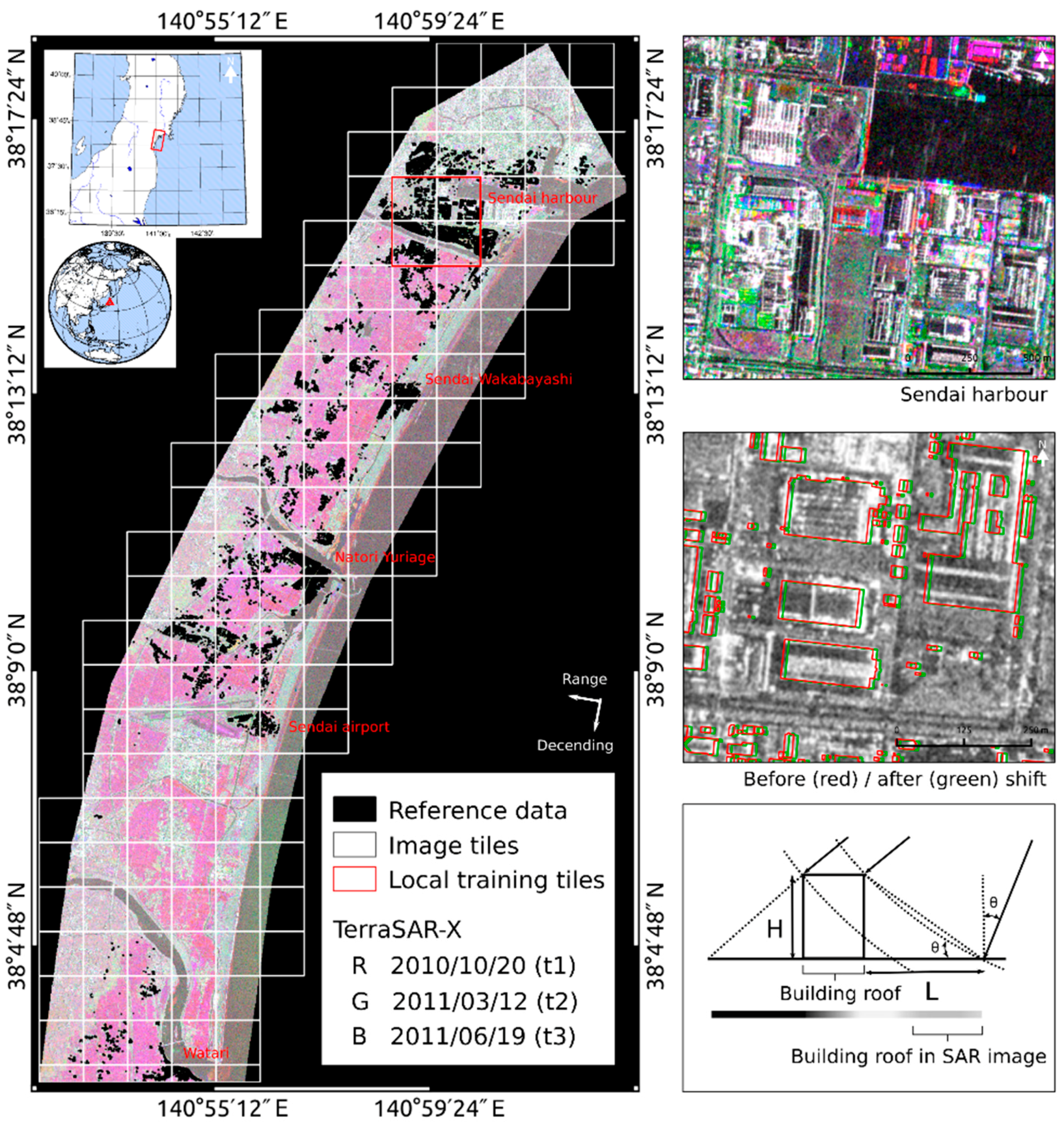
The study focuses on the coastal areas of the Southern Miyagi prefecture in Japan (
Figure 1 left), which was amongst the most severely affected regions hit by a Mw 9.0 earthquake and subsequent tsunami on 11 March 2011. The earthquake led to significant crustal movement over large areas and caused a tsunami with maximum run-up of 40.1 m [
26]. Major damages to buildings, infrastructure and the environment occurred and a large number of people were reported dead or missing.
Three X-band images from the TerraSAR-X sensor taken five months before (t1), as well as one day (t2) and three months (t3) after the disaster were acquired over the study area (
Table 1).
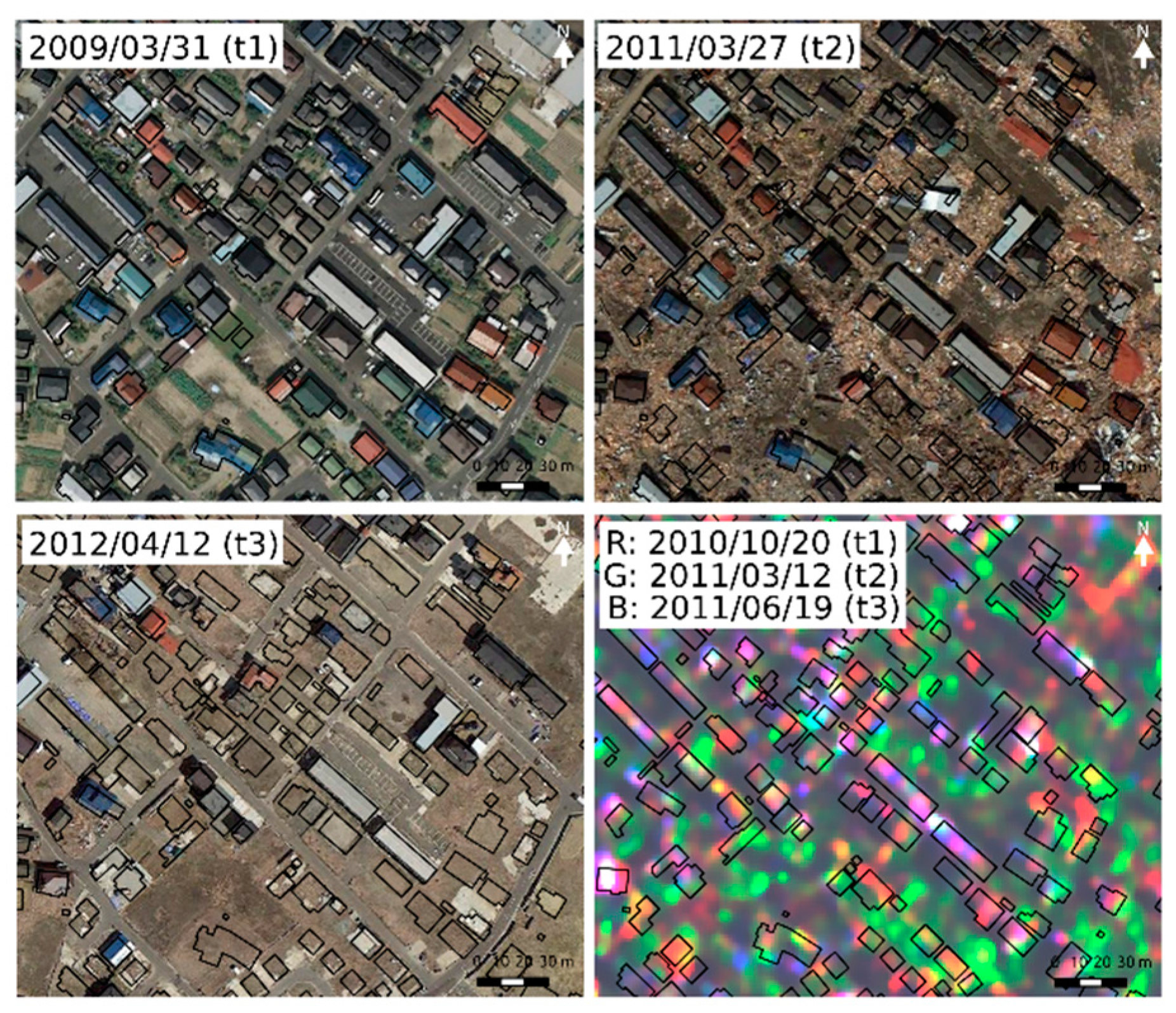
Figure 1 (left and upper right) shows a false-color composite of the TerraSAR-X images that highlights the differences in backscattering intensities between the different acquisition times. The images were captured in StripMap mode with HH polarization on a descending path with 37.3° incidence angle and delivered as Single Look Slant Range Complex (SSC) products. Two L-band images of the ALOS PALSAR sensor with HH polarization on a descending path with 34.3° incidence angle, taken five months before (t1) and one month (t2) after the disaster were acquired and delivered at processing level 1.1 (
Table 1). Image preprocessing steps for both image types included multi-look focusing (with four equivalent number of looks), orthorectification (UTM 54N/WGS84), resampling, radiometric correction and conversion of digital numbers to sigma naught (db). Co-registration to the pre-event images has been performed using an algorithm based on Fast Fourier Transform (FFT) for translation, rotation and scale-invariant image registration [
27]. No speckle filtering has been applied.
Comprehensive reference data are used in this study from a database of building damages that were surveyed by the Japanese Ministry of Land Infrastructure, Transport and Tourism after the disaster [
28]. The data are referenced at the building footprint and include 18,407 buildings described by seven damage categories. Two reclassifications of the data have been performed as is depicted in
Table 2. An overview of potential tsunami damage patterns and their characteristics in SAR imagery can be found in [
23]. The building geometries have, moreover, been shifted to match the building outlines in the SAR images.
Figure 1 (middle, right) shows the original building geometries in red and the shifted ones in green over the pre-event image (t1) for TerraSAR-X. Parts of the building walls with highest backscatter from corner reflection are outside the original footprints for most of the buildings. This can be attributed largely to the fact that a building in a TerraSAR-X image shows layover from the actual position to the direction of the sensor (
Figure 1 bottom, right). The layover (
L) is proportional to the building height (
H) and can be calculated as
where
θ is the incident angle of the microwave. In order to account for this effect, the building geometries were shifted towards the direction of the sensor to match the TerraSAR-X images. With
θ = 37.3° and an assumed average building height of
H = 6 m (approximately the height of a two-storied building), the layover is approximately 7.9 m. The assumption that the majority of the buildings in the study area have two stories is based on field work as described in Liu et al. [
11]. Considering the path of the satellite (190.4° clockwise from north), the layover can be decomposed into 7.8 m to the east and 1.4 m to the south, which results in a lateral shift of the building geometries of 6 px to the east and 1 px to the south on the basis of a resampled pixel spacing of 1.25 m. Comparing the adjusted building geometries with the original ones (
Figure 1 middle, right) larger areas of high backscattering intensities are located within the building footprints. Similarly, a copy of the reference data was shifted for the ALOS imagery according to incidence angle and path of the satellite by 8.7 m to the east and 1.6 m to the south.
Preprocessing of the satellite images has been performed with the Sentinel-1 Toolbox. Co-registration and all other processing and analysis steps have been implemented in Python using the GDAL, NumPy, SciPy and Scikit-learn libraries.
5. Discussion
The study showed that major changes to the building stock are clearly described by the backscattering intensities of X- and L-band SAR images and can be detected by a trained and tuned SVM learning machine. A number of research questions have been considered and are discussed in the following in order to give guidance on how to train a powerful SVM for change detection.
(1) How do the training samples influence the change detection performance?
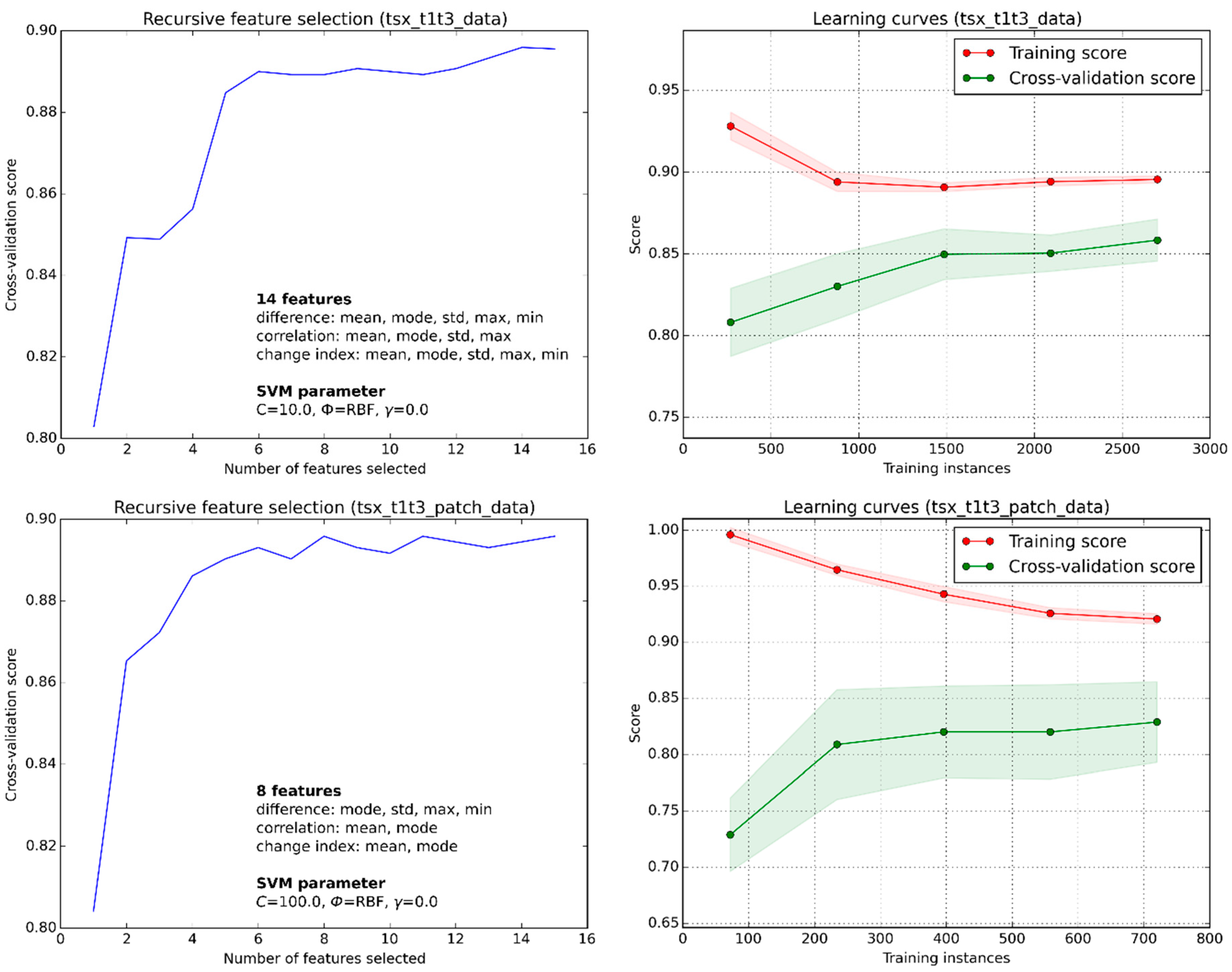
Given a large enough training sample size (>750 samples per class), good generalization ability of the SVM at high accuracy level (>0.85 F1 score) could be observed (
Figure 4, top). Even when reducing the training sample size to 400 samples per class, good classification accuracy (>0.83 F1 score) could be measured when trained and tested over the whole study area. The learning curves indicate that further reducing the sample size to as low as 100 samples per class could still provide reliable results (>0.80 F1 score), albeit at the cost of losing generalization ability. To this regard, we could also show that it is possible to apply a locally trained classifier to different areas (
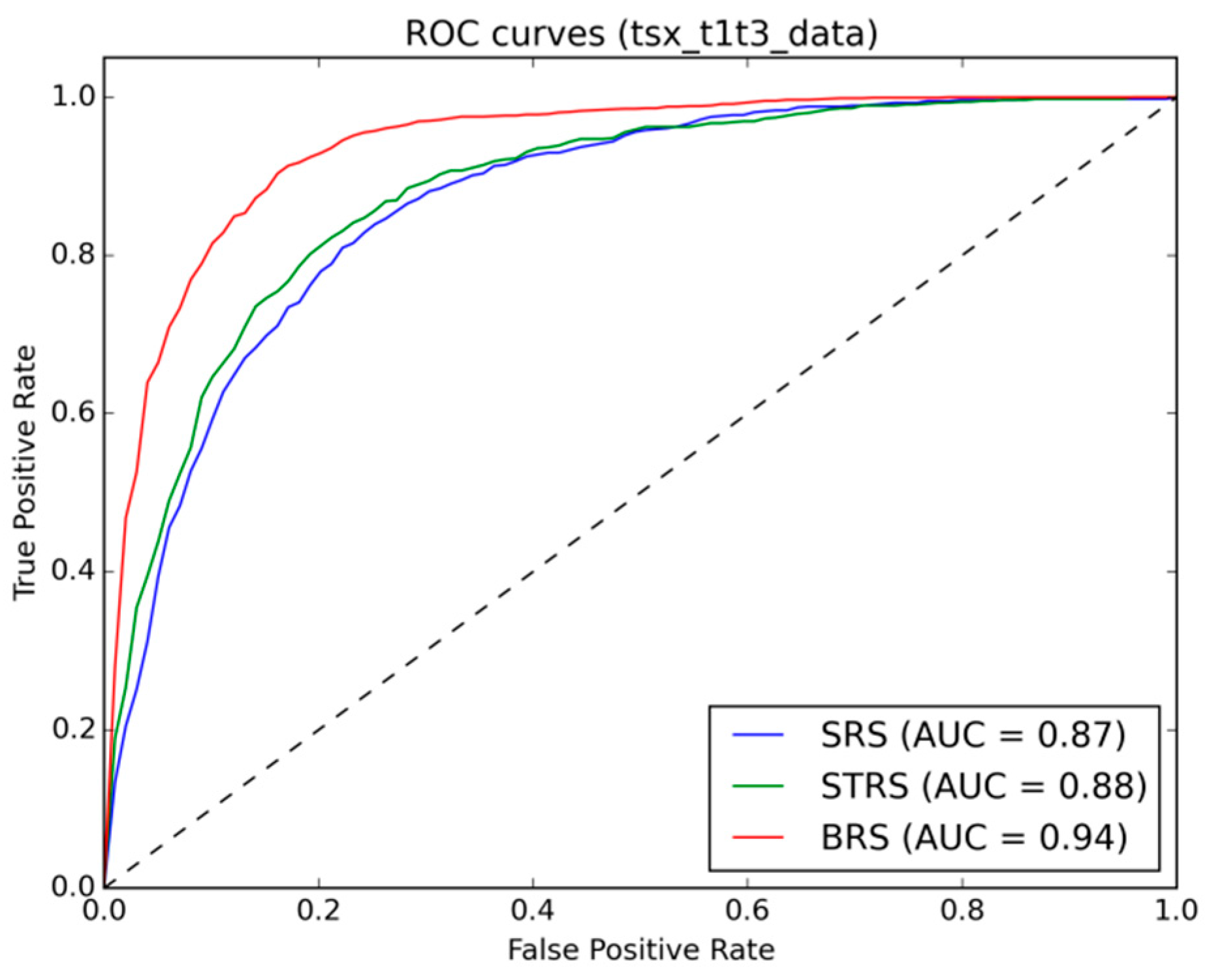
Table 4) with minor loss of performance (0.78 F1 score) compared to a classifier that has been trained over the whole image scene (0.85 F1 score). The generalization experiment carried out in this study, however, could only be applied within the same image scene. Therefore, further tests involving different scenes are needed to strengthen and further constrain these findings. The training sample approach had a clear impact on the results, and a balanced random sample of training data produced superior results (0.85 F1 score) over stratified (0.73 F1 score) or simple random samples (0.73 F1 score). This confirms the sensitivity of SVM to class imbalance as also observed in other classification domains [
35] (
Table 3). An alternative strategy to account for the class imbalance is to use the prior class distribution, as estimated from the training samples, to weight the penalty parameter
C during classification. An in-depth discussion on imbalanced learning can be found in He and Ma (2013) [
36].
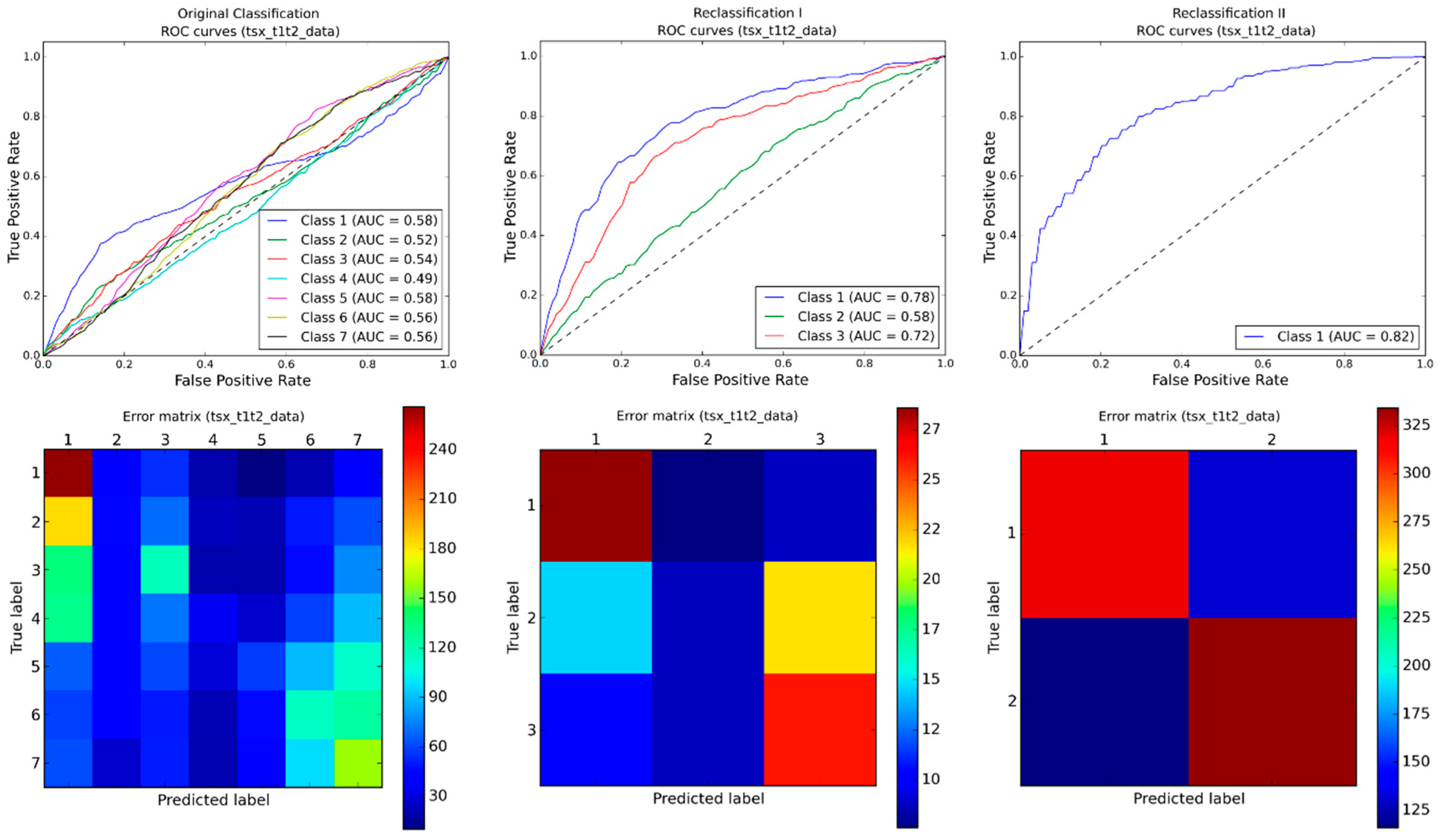
(2) How many change classes can be distinguished?
The classifier performed well in case of a simple binary classification task (change−no change). Given the tested feature space and classification approach, a distinction between different types of changes in terms of damage grades led to poor performance of the classifier. The types of changes that are related to tsunami-induced damages represent a major difficulty to be detected by satellite images in general, since they occur mainly in the side-walls of the structures and not the roof. Yamazaki et al. (2013) [
37] present an approach to tackle that problem by utilizing the side-looking nature of the SAR sensor. Their results seem promising for single buildings. Given the scenario and approach followed within the study at hand, however, such changes could not be detected in a robust manner over a large number of buildings. To this regard, additional change features such as texture, coherence and curvelet features [
7,
38] should be tested in more depth.
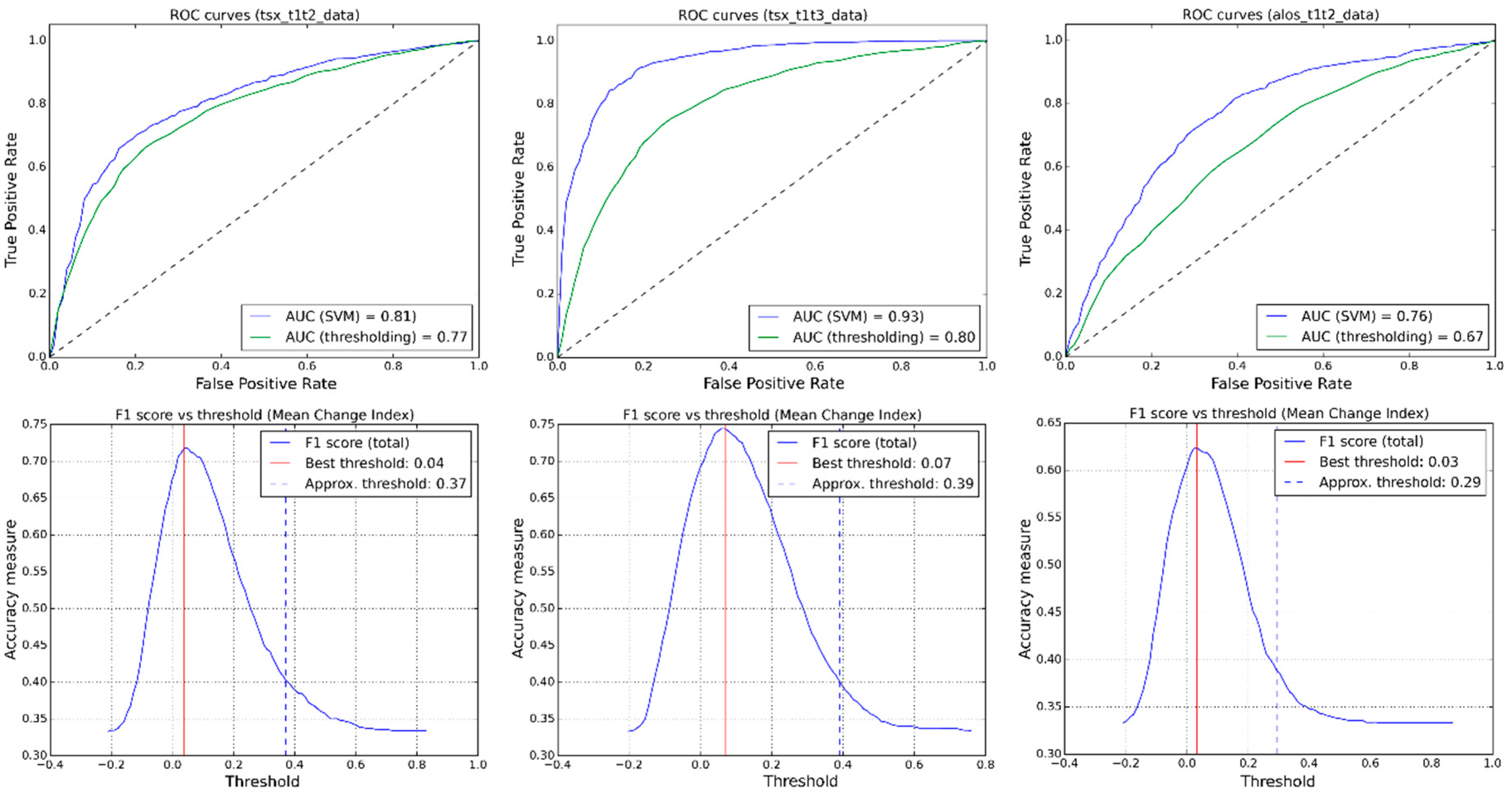
(3) How does the choice of the acquisition dates influence the detection of changes?
Different image acquisition dates have been tested for their influence on the classification performance (
Figure 6,
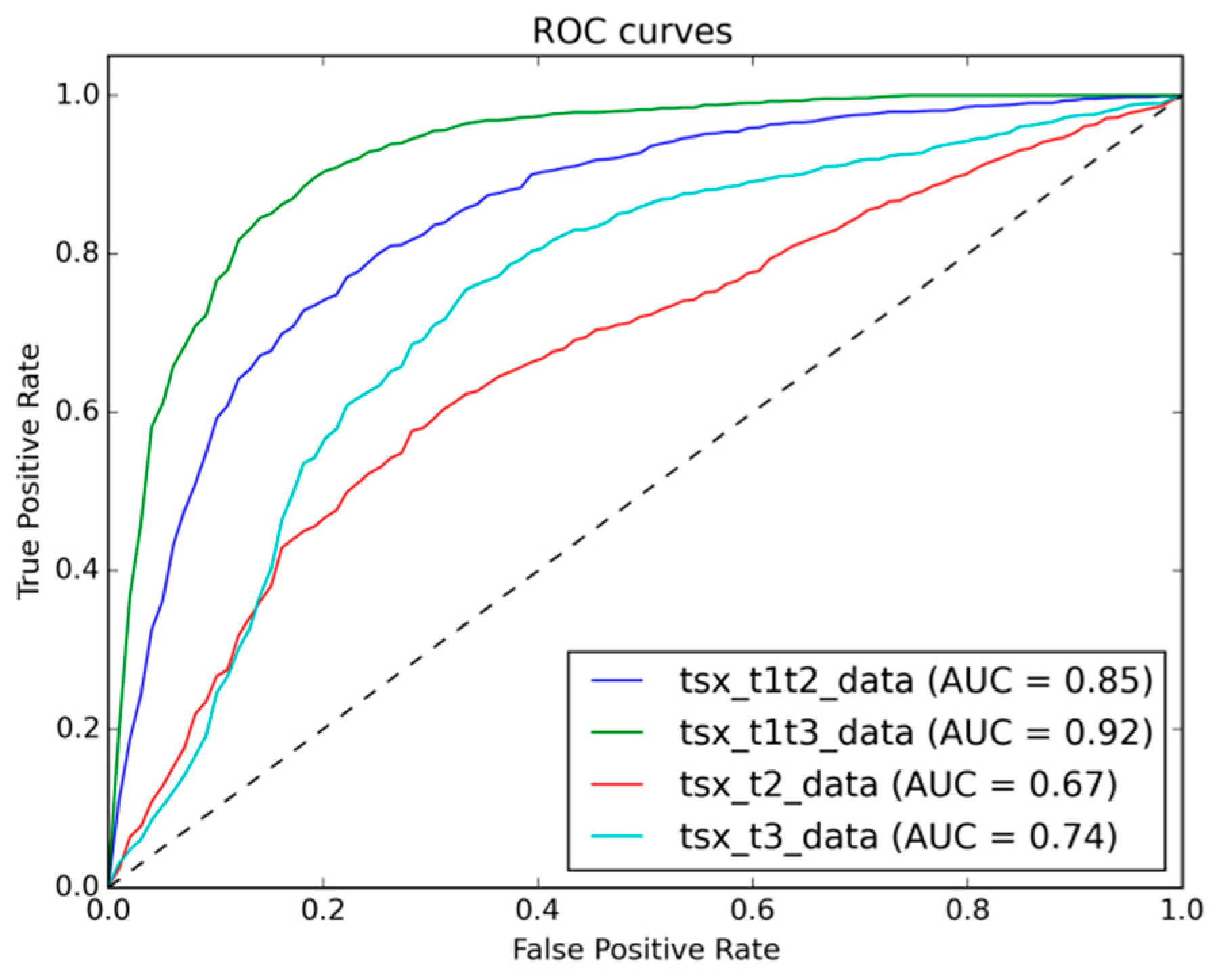
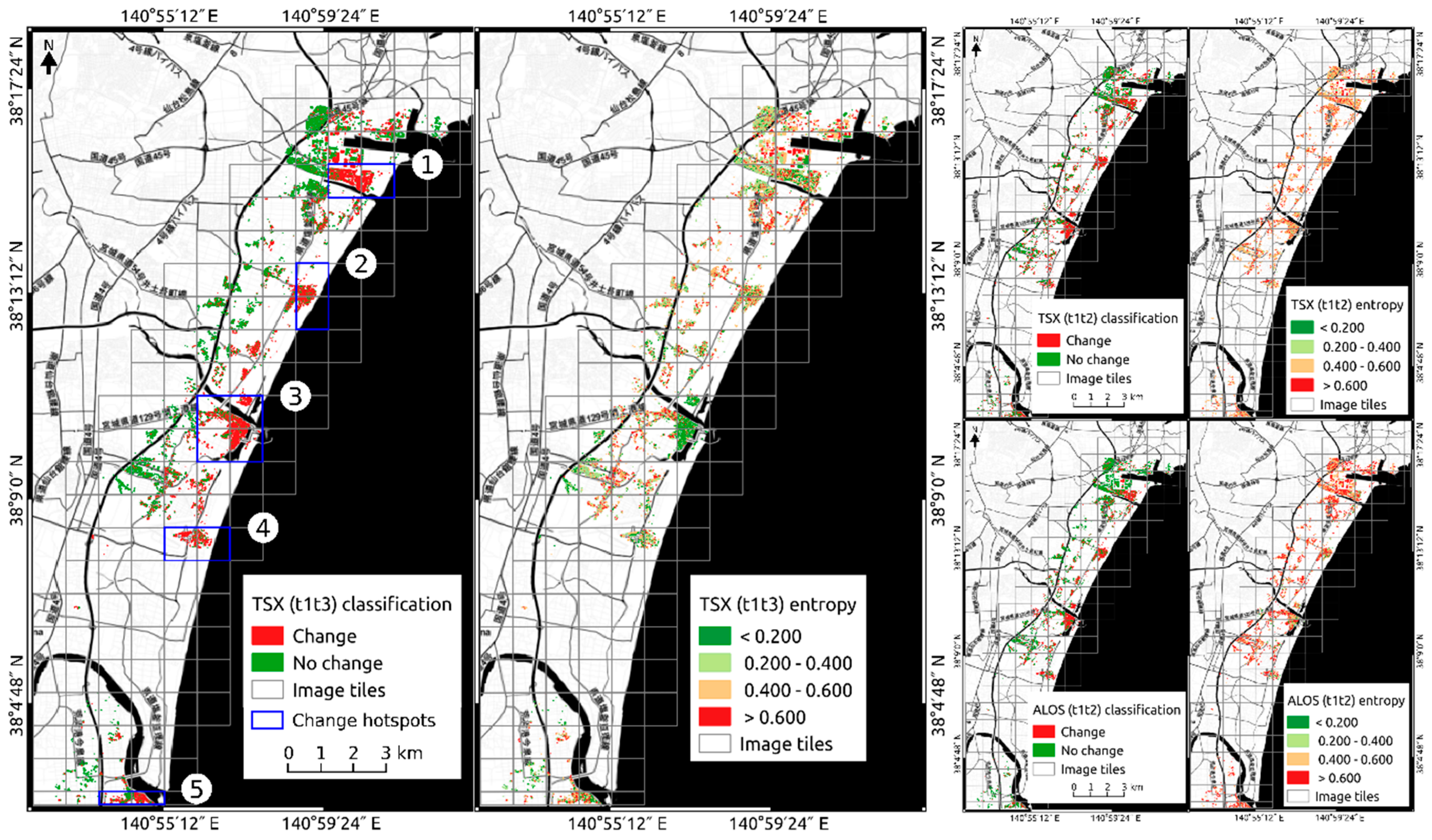
Table 5). The best results were observed on the t1t3 image pair (0.92 AUC), which uses a post-event image acquired three months after the disaster where large amounts of debris and collapsed buildings had already been removed. Image pairs that utilize shorter acquisition dates after the event (one day for TSX) showed a performance decrease (0.85 AUC). One reason for this is that, in many cases where the reference data reports a total collapse, only the lower floors of structures are damaged by the tsunami, whereas the roofs do not show any apparent changes from the satellite’s point of view. As can be seen from
Figure 5, these buildings are still present in the image acquired immediately after the disaster, but were then removed as part of the clean-up activities in the weeks after the disaster. Therefore, the aforementioned limitations related to the viewpoint of satellite-based change detection are further confirmed by this experiment and it could be shown that this becomes particularly important for any change detection application that aims at providing immediate post-disaster situation awareness.
A benefit of the proposed supervised change detection approach is that once training samples are defined and labelled according to the desired classification scheme, basically any change feature space can be processed without further adjustments. In this regard, also single date classifications that use only one post-disaster image have been successfully tested within the same framework. Classification of the mono-temporal feature space could achieve reasonably good performance on both t2 (0.67 AUC) and t3 (0.74 AUC) images that, however, could not compete with the multi-temporal approach (t1t2 image pair: 0.85 AUC; t1t3 image pair 0.92 AUC). It shows, nevertheless, that the proposed approach is flexible enough to deal with a multitude of possible data availability situations in case of a disaster.
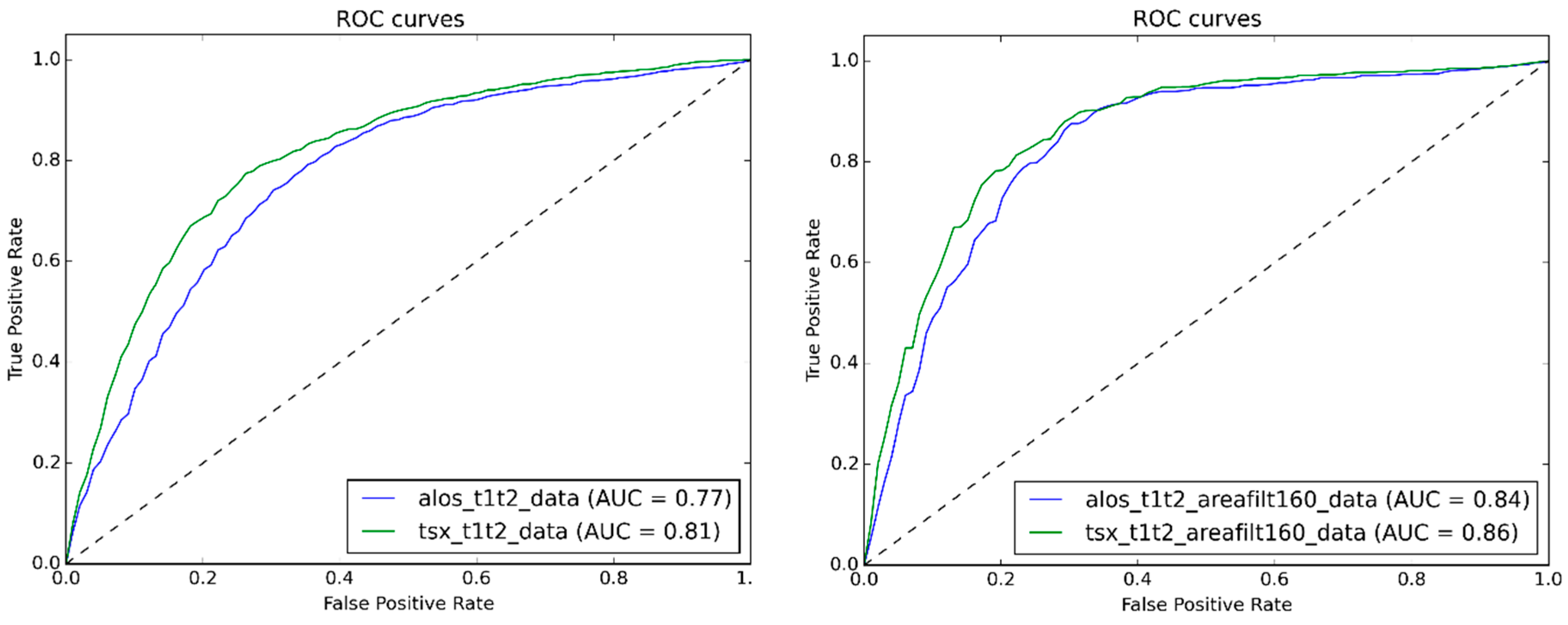
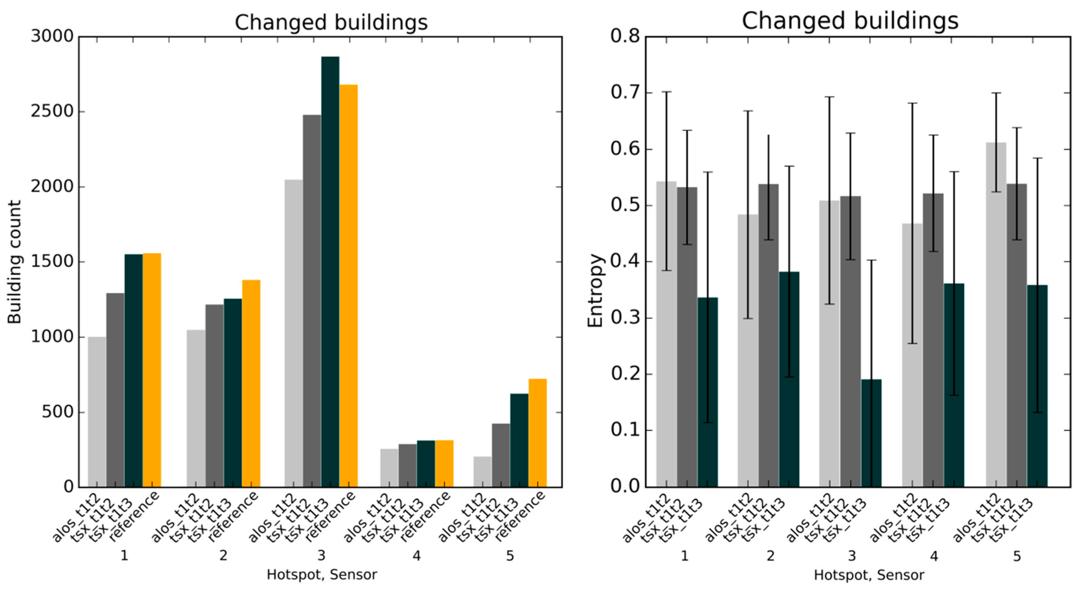
(4) How do X-band and L-band SAR compare for the detection of changes?
The flexibility of the approach is further emphasized by the fact that it could successfully be applied to both X- and L-band images. A comparison of SVM on X- and L-band images showed slightly better performance of TSX (0.81 AUC) than ALOS (0.77 AUC). Also a test, for which only buildings with a footprint of larger than 160 m² were considered to account for the lower spatial resolution of ALOS, indicated an almost negligible performance difference (0.02 AUC). When looking at the final results over the whole study area it can be seen that the ALOS L-band tends to significantly underestimate the number of changed buildings. This is likely to be related to the characteristics of the ALOS L-band, which compared to the TSX X-band shows low backscatter intensity in dense residential areas. It may thus negatively affect the detection rate of damaged houses with small intensity changes. Even though the acquisition dates of ALOS and TSX were selected as close as possible to each other, still the t2 images are 26 days apart from each other. In order to avoid a possible bias by real-world changes that may have occurred during this difference period, further tests with closer acquisition dates should be carried out.
(5) How does an SVM compare to thresholding change detection?
The proposed machine learning approach performed significantly better than a thresholding change detection over all tested training-testing scenarios and thresholds (
Figure 9,
Table 6). Testing of the thresholding approach has been carried out over all possible thresholds in order to avoid bias by a particular threshold approximation method. Also comparing the change detection resulting from the best threshold over all iterations with the results obtained from a trained SVM showed superior performance of SVM with respect to thresholding on all image types and acquisition dates. The window of possible thresholds that yield comparable results is, moreover, narrow and could not be identified by a simple threshold approximation method (
Figure 9).
(6) Other considerations
Different kernel functions have been used within this study and were optimized for each classification by means of cross-validation and grid-search. For most of the classifications a radial basis function has been selected by the optimization procedure. Even though the influence of kernel functions and other SVM parameters on the performance of the change detection has not specifically been evaluated by this study, it is significant as has been shown by, for example, Camps-Valls [
21] and should be considered by any study attempting to use SVM for change detection on SAR imagery.
Using an object-based approach with external building footprint data as computational unit needs to account for the SAR image geometry. Therefore, footprints should be adjusted accordingly before further analysis, which was done in this study by shifting them laterally. In case no independent building footprint data are available, the influence of the image segmentation on the classification performance should be evaluated more specifically as it can potentially have a significant impact on the classification [
25].
6. Conclusions
This study evaluated the performance of a Support Vector Machine (SVM) classifier to learn and detect changes in single- and multi-temporal X- and L-band Synthetic Aperture Radar (SAR) images under varying conditions. The apparent drawback of a machine learning approach to change detection is largely related to the often costly acquisition of training data. With this study, however, we were able to demonstrate that given automatic SVM parameter tuning and feature selection, in addition to considering several critical decisions commonly made during the training stage, the costs for training an SVM can be significantly reduced. Balancing the training samples between the change classes led to significant improvements with respect to random sampling. With a large enough training sample size (>400 sample per class), moreover, good generalization ability of the SVM at high accuracy levels (>0.80 F1 score) can be achieved. The experiments further indicate that it is possible to transfer a locally trained classifier to different areas with only minor loss of performance. The classifier performed well in the case of a simple binary classification task, but distinguishing more complex change types, such as tsunami-related changes that do not directly affect the roof structure, lead to a significant performance decrease. The best results were observed on image pairs with a larger temporal baseline. A clear performance decrease could be observed for single-date change classifications based on post-event images with respect to a multi-temporal classification. Since the overall performances are still good (>0.67 F1 score) such a post-event classification can be a useful approach for the case when no suitable pre-event images are available or when very rapid change assessments need to be carried out in emergency situations. A direct comparison of SVM on X- and L-band images showed better performance of TSX than ALOS. Over all training and testing scenarios, however, the difference is minor (0.04 AUC). Compared to thresholding change detection, the machine learning approach performed significantly better on the tested image types and acquisition dates. This conclusion holds independent on the selected threshold approximation approach.
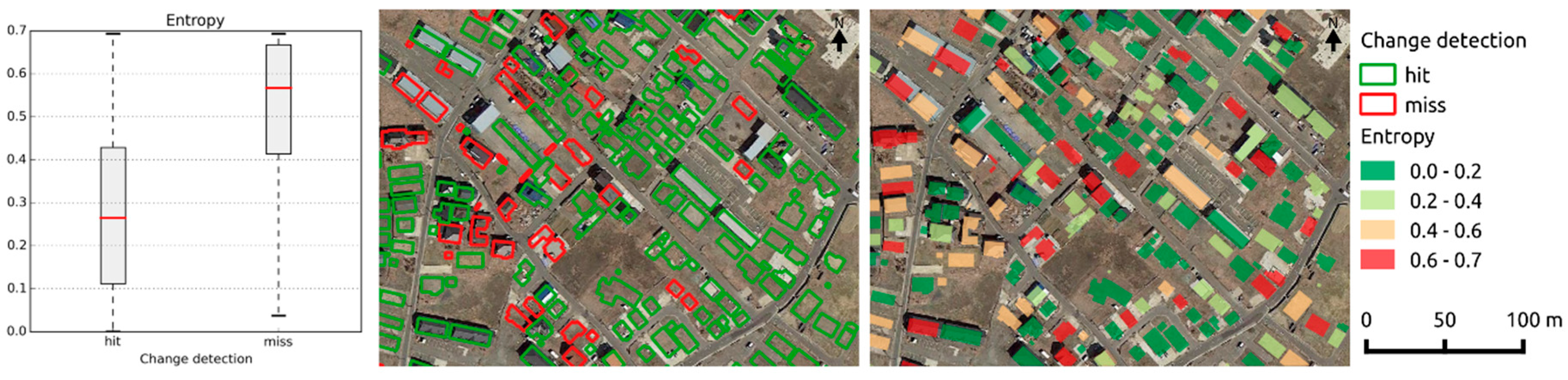
The benefits of a machine learning approach lie mainly in the fact that it allows a partitioning of a multi-dimensional change feature space that can provide more diverse information about the changed objects with respect to a single feature or a composed feature index. Also, the definition of the decision boundary by selection of relevant training samples is more intuitive from a user’s perspective than fixing a threshold value. Moreover, the computation of Shannon entropy values from the soft answers of the SVM classifier proved to be a valid confidence measure that can aid the identification of possible false classifications and could support a targeted improvement of the change maps either by means of an active learning approach or by manual post-classification refinement. In case of a disaster, the proposed approach can be intuitively adjusted to local conditions in terms of applicable types of changes which may vary depending on the hazard type, the geographical region of interest and the objects of interest. Such an adjustment would commonly involve visual inspection of optical imagery from at least a subset of the affected area in order to acquire training samples. Detailed damage mapping as part of the operational emergency response protocols is largely done by human operators based on visual inspection of very high resolution optical imagery [
39]. Thus, the findings of this study can be used to design a machine learning application that is coupled with such mapping operations and that can provide regular rapid estimates of the spatial distribution of most devastating changes while the detailed but more time-consuming damage mapping is in progress. The estimates from the learning machine can be used to guide and iteratively prioritize the manual mapping efforts. An example of a similar approach to prioritize data acquisition in order to improve post-earthquake insurance claim management is given in Pittore et al. [
40].
Ongoing and future research efforts focus on extending the change feature space by texture, coherence and curvelet features [
7,
38] on testing the transferability of trained learning machines across image scenes and detection tasks, on further comparisons of the proposed method with other kernel-based methods [
21,
24] and on developing a prototype application for iterative change detection and mapping prioritization.


