Earthquake-Induced Building Damage Detection with Post-Event Sub-Meter VHR TerraSAR-X Staring Spotlight Imagery

Abstract

Compared with optical sensors, Synthetic Aperture Radar (SAR) can provide important damage information due to its ability to map areas affected by earthquakes independently from weather conditions and solar illumination. In 2013, a new TerraSAR-X mode named staring spotlight (ST), whose azimuth resolution was improved to 0.24 m, was introduced for various applications. This data source made it possible to extract detailed information from individual buildings. In this paper, we present a new concept for individual building damage assessment using a post-event sub-meter very high resolution (VHR) SAR image and a building footprint map. With the building footprint map, the original footprints of buildings can be located in the SAR image. Based on the building imaging analysis of a building in the SAR image, the features in the building footprint can be extracted to identify standing and collapsed buildings. Three machine learning classifiers, including random forest (RF), support vector machine (SVM) and K-nearest neighbor (K-NN), are used in the experiments. The results show that the proposed method can obtain good overall accuracy, which is above 80% with the three classifiers. The efficiency of the proposed method is demonstrated based on samples of buildings using descending and ascending sub-meter VHR ST images, which were all acquired from the same area in old Beichuan County, China.

1. Introduction

Damage detection after earthquakes is an important issue for post-disaster emergency response, impact assessment and relief activities. Building damage detection is particularly crucial for identifying areas that require urgent rescue efforts. Remote sensing has shown excellent capability for use in rapid impact assessments, as it can provide information for damage mapping in large areas and in an uncensored manner, particularly when information networks are inoperative and road connections are destroyed in areas impacted by earthquakes. Compared with optical sensors, Synthetic Aperture Radar (SAR) can provide important damage information due to its ability to map affected areas independently from the weather conditions and solar illumination, representing an import data source for damage assessment.

Many approaches for damage detection with SAR imagery have been introduced [1,2]. Change detection with pre- and post-event SAR images is widely used for damage assessment, and it has become a standard procedure [3]. The differences between the backscattering intensity and intensity correlation coefficients of images before and after earthquakes indicate potential damage areas. In addition, the interferometric coherence of pre- and post-event SAR data can also provide important information for damage assessment [1]. In the case of change detection, the pre- and post-event data are needed for comparison. However, in many areas, almost no archived SAR images, especially for high-resolution SAR data, are available. Therefore, research on building damage assessment with only post-event SAR images is necessary.

The new generation of high-resolution SAR satellite systems was first deployed for earthquake monitoring during the Wenchuan Earthquake in 2008 [3]. Meter-resolution SAR images from TerraSAR-X and COSMO-SkyMed were acquired for damage assessment. Although the image resolution has improved, it is difficult to identify collapsed buildings using single meter-resolution SAR images [3,4]. After 2013, a new TerraSAR-X mode named staring spotlight (ST), whose azimuth resolution was improved to 0.24 m, was introduced. The sub-meter very high resolution (VHR) SAR data source provides new opportunities for earthquake damage mapping because more details can be observed in images, making it possible to focus an analysis on individual buildings.

Previous works have generally concentrated on the building block level of damage assessment with low- or medium-resolution SAR images. Few studies have focused on individual buildings due to lack of VHR SAR images. Balz et al. [3] analyzed the appearances of destroyed and partly destroyed buildings using high-resolution SAR images and proposed a technical workflow to identify building damage using post-seismic high-resolution SAR satellite data. Another method was developed to detect building damage in individual building units using pre-event high-resolution optical images and post-event high-resolution SAR data based on the similarity measurement between simulated and real SAR images [5]. Wang et al. [6] proposed an approach for post-earthquake building damage assessment using multi-mutual information from pre-event optical images and post-event SAR images. Brunner et al. [4] analyzed a set of decimeter-resolution SAR images of an artificial village with different types of destroyed buildings. The analysis showed that the decimeter-resolution SAR data are fine enough to classify building signatures according to basic damage classes. Kuny et al. [7] used simulated SAR images of different types of building damage for feature analysis and proposed a method for discriminating between debris heaps and high vegetation with simulated SAR data and TerraSAR-X images [8]. Wu et al. [9,10] analyzed different building damage types in TerraSAR-X ST mode data by visual interpretation, statistical comparison and classification assessment. The results showed that the data effectively separated standing buildings from collapsed buildings. However, the damaged building samples were obtained by expert interpretation and manual extraction. This method is time consuming and technique dependent because the exact edges of buildings and debris must be acquired.

In sub-meter VHR SAR images, more features, such as points and edges of objects, become visible, more details of individual buildings can be observed and new features of buildings are shown [11]. It is difficult to detect specific buildings in complicated surroundings in VHR images. Moreover, collapsed building debris is visually similar to other objects such as high vegetation [8]. This could lead to false alarms when detecting debris heaps.

Therefore, in this paper, we propose a method to assess the damage to individual buildings affected by earthquakes using single post-event VHR SAR imagery and a building footprint map. Given a building footprint map, which can be provided by a cadastral map or extracted from a pre-event VHR optical image, the original footprints of buildings can be located in the geometrically-rectified post-event VHR SAR image. Because collapsed and standing buildings exhibit different characteristics in their original footprints, features can be extracted from the image. Then, the buildings can be classified as different damage types. We demonstrate the feasibility of the proposed method in Qushan town (31.833°N, 104.459°E), old Beichuan County, China, which was heavily damaged in the Wenchuan Earthquake on 12 May 2008. The ruins in the area are preserved as the Beichuan Earthquake Memorial Park. Therefore, some damaged buildings in the area can be used for algorithm analysis. In our experiments, the post-event descending and ascending TerraSAR-X ST data are used for building damage assessment. Post-event airborne optical images, light detection and ranging (LIDAR) data, as well as in situ photography are used as reference data. The main novelty of the paper is the use of the VHR TerraSAR-X ST data for individual damage building analysis and demonstrating the concept for collapsed building assessment with building footprints.

The remainder of this paper is structured as follows. In Section 2, the properties of damaged buildings in VHR SAR images and damage detection problems are stated. In Section 3, we introduce the basic principle of the proposed method and describe damage detection with sub-meter VHR SAR data in detail. The study area and dataset are introduced in Section 4. Section 5 gives the results and analysis of the experiments. Finally, the discussion and conclusions are presented in Section 6 and Section 7, respectively.

2. Properties of Damaged Buildings in VHR SAR Images and Damage Detection Problems

Due to the side-looking image mode of SAR sensors, some unique features, such as layover, fore-shortening effects and multi-path propagation, can be observed in SAR images. Those effects make interpretation with SAR images difficult compared to using optical images. However, the effects are also the unique patterns of buildings, which can be differentiated from other objects in SAR images.

In general, buildings have very distinct appearances in SAR images due to their cube-like or regular shapes. Buildings in SAR images typically consist of four zones: a layover area, corner reflection, roof area and shadow area. When an earthquake occurs, buildings may be destroyed or collapse. Destroyed buildings have different scattering distributions. Strong double-bounce scattering may be missing because the vertical wall facing the sensor may be collapsed, and the wall-ground dihedral corner reflector may be destroyed. The layover area may also be missing. Furthermore, the shadow area of a building will be reduced and potentially missing, depending on the structure and slope of the ruins.

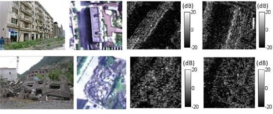
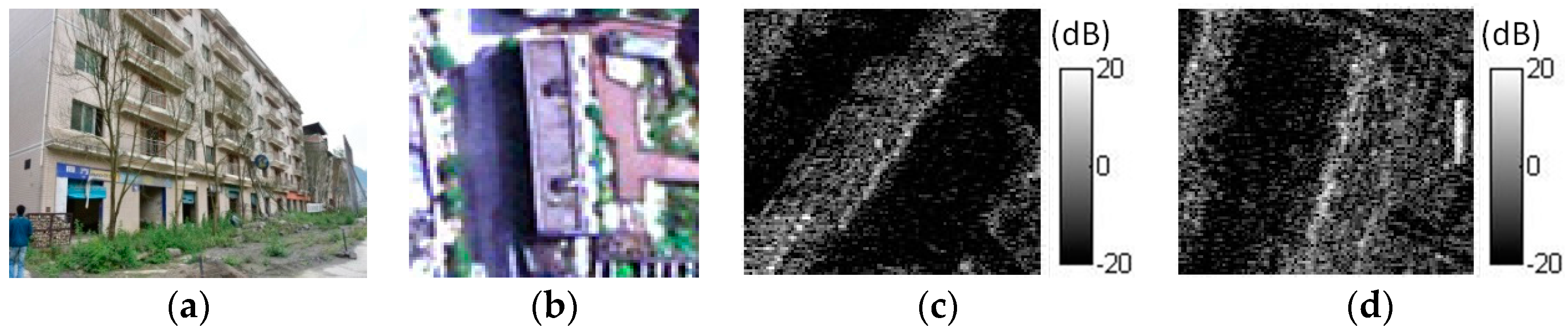
Figure 1 illustrates a standing building after an earthquake. Figure 1a is an in situ photograph; Figure 1b is an optical image; and Figure 1c,d show the building in ascending and descending TerraSAR-X ST mode SAR images, respectively. The azimuth direction of Figure 1c is from bottom to top, and the range direction is from left to right. The azimuth direction of Figure 1d is from top to bottom, and the range direction is from right to left. The building has a flat roof with slight damage. In the SAR image, the double-bounce line, layover area and shadow area are obvious. The layover areas can be detected as the areas facing the sensor. The shadow areas are distinguishable from their surroundings.

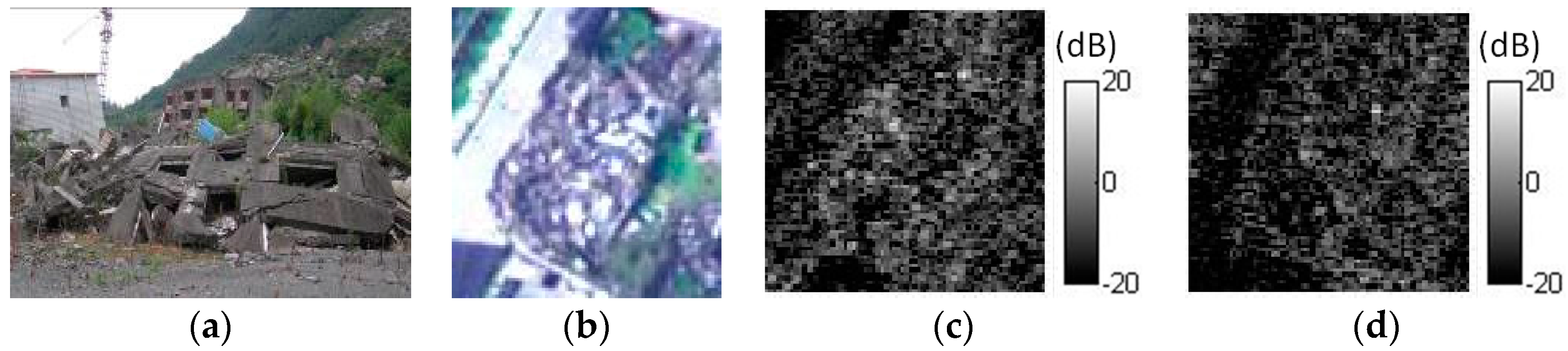
Figure 2 illustrates a totally collapsed building after an earthquake. Figure 2a is an in situ photograph; Figure 2b is an optical image; and Figure 2c,d show the building in TerraSAR-X ST ascending and descending SAR images, respectively. The azimuth direction of Figure 2c is from bottom to top, and the range direction is from left to right. The azimuth direction of Figure 2d is from top to bottom, and the range direction is from right to left. The damaged building was collapsed entirely, leaving a heap of randomly-oriented planes mainly made of concrete. In the SAR image, the heap of debris of the collapsed building shows random scattering effects. Some bright scattering spots can be found, which are caused by corner reflectors, resulting from the composition of different planes. However, the double-bounce line, layover area and shadow area are missing in this case.

Thus, in Figure 1 and Figure 2, we can see that the standing building and the totally collapsed building have their own unique features in the VHR SAR images. However, high vegetation shows features that are similar to those of the debris of the totally collapsed building and may cause false alarms [8]. Moreover, it is not easy to extract the exact edges of the debris due to the similarity between the debris and surroundings. Therefore, although the signature of the standing building shows different features compared to those of the collapsed building in the VHR SAR images, detecting the collapsed building debris using only post-event VHR SAR images by the traditional image processing method remains problematic. Overcoming this issue is the motivation of the paper.

3. Proposed Methodology for Damage Detection Using VHR SAR Images

3.1. Concept of Damage Detection

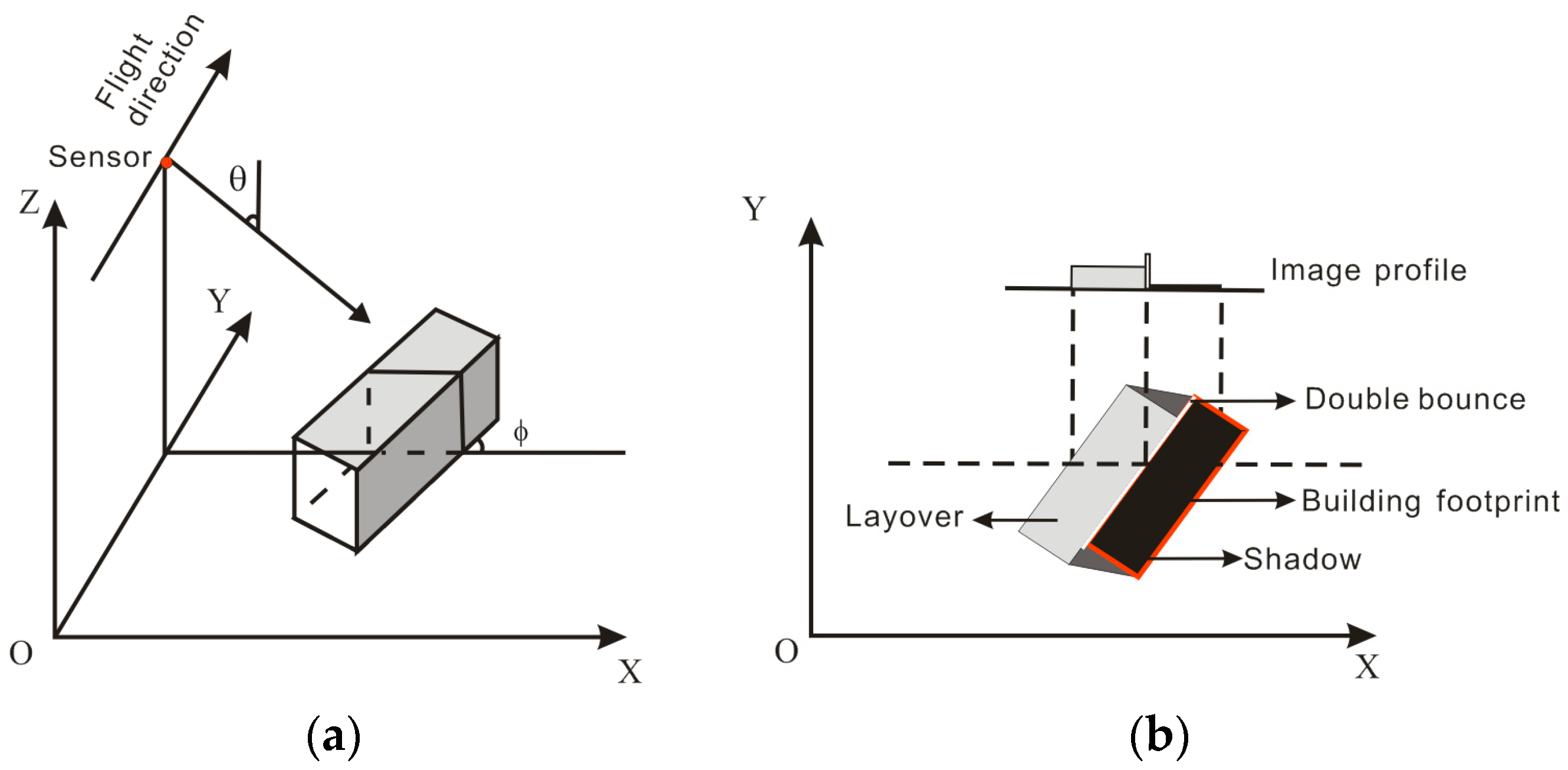
Figure 3 gives an ideal example of SAR imaging of a flat roof building. In Figure 3b, the layover, double-bounce line and shadow area can be observed. The shadow caused by the standing building covers the majority of the building’s footprint (denoted by the red line). Generally, there is no return from the building or the ground in the shadow area. Therefore, the backscattering intensity in the area is lower than that in the surrounding area.

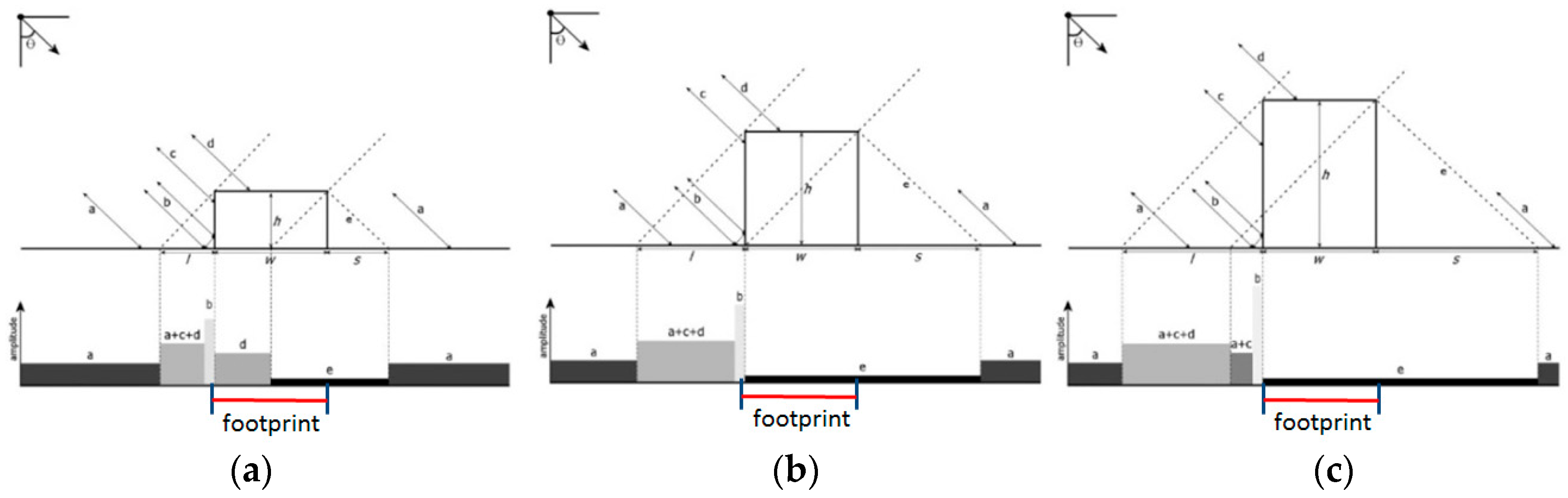
For further investigation, Figure 4 and Figure 5 show examples of the backscattering range profiles of flat roof and gable roof buildings under different boundary conditions [12]. In Figure 4, the scattering effects of flat roof buildings for three different situations can be observed according to the boundary conditions among the building height h, width w and incidence angle θ (Figure 4a–c). The symbols l and s denote the lengths of the layover and shadow in the ground-projected image space, respectively; b is the double bounce caused by the dihedral corner reflector formed by the vertical wall of the building and the surrounding ground; and e represents the shadow area from which there is no return from the building or the ground. In Figure 4, some regularity can be observed. The double bounce always appears as a linear feature corresponding to the building’s front wall, and it can indicate the presence of a building. Near the double bounce, the shadow areas (e in Figure 4b,c) usually appear in the image and cover the area of the building’s footprint. In Figure 4a, there is backscattering return from the roof between the double bounce and shadow. If the roof is flat, minimal backscattering from the roof is received by the sensor. Thus, d (backscattering from the roof) in Figure 4a usually appears as a dark region in SAR images. 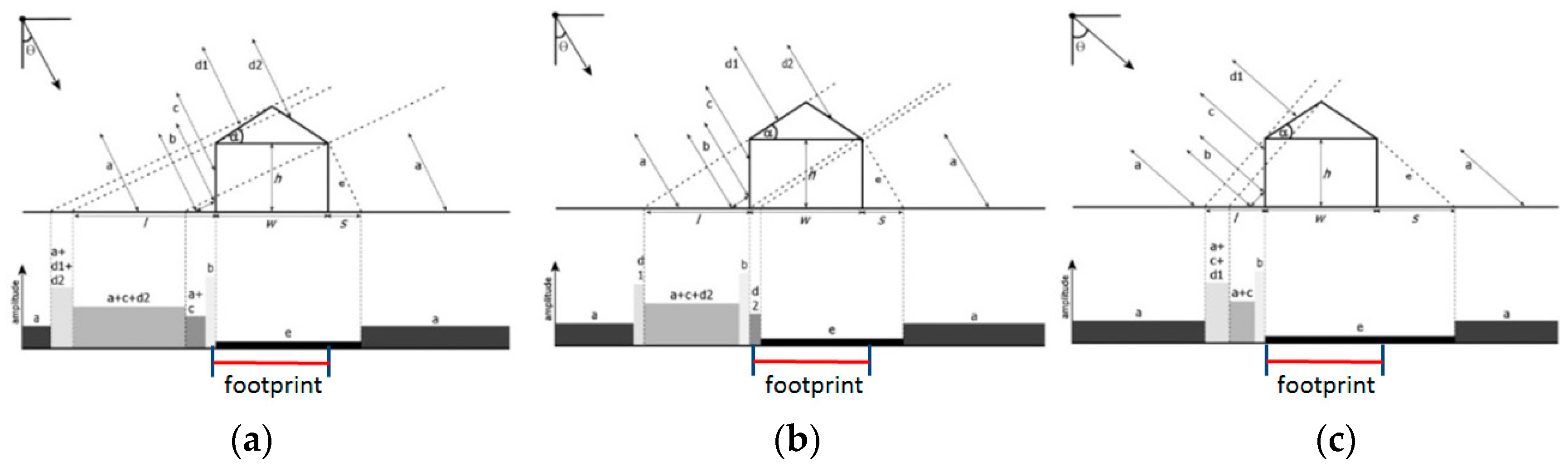Figure 5 shows the scattering effects of a gable roof building. It shows three examples of backscattering profiles from a gable roof building with roof inclination angles α for different incidence angles θ. Near the double-bounce line, the shadow areas (e in Figure 5) also cover the majority of the building’s footprint.

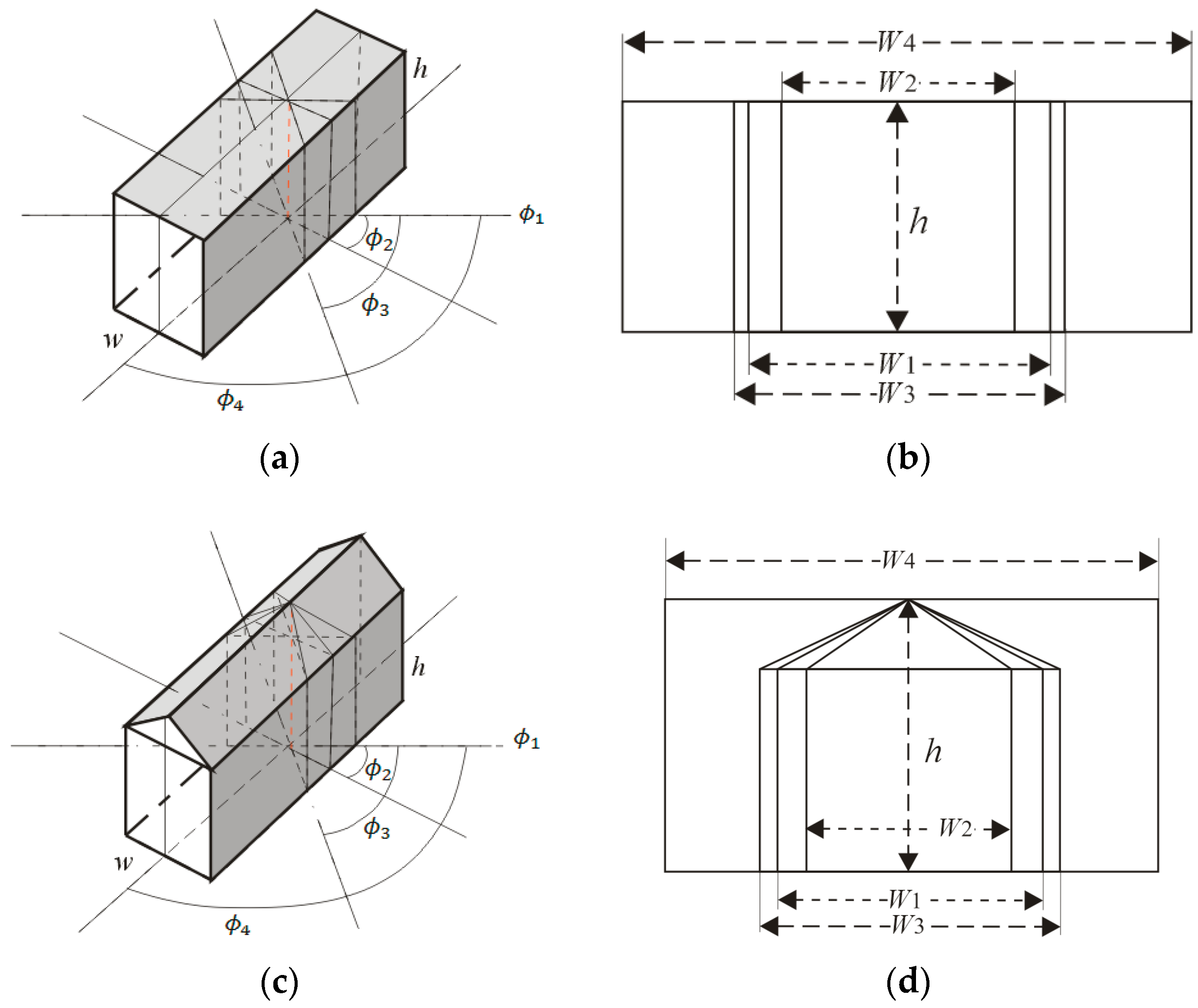
Generally, for a flat or gable roof building, no matter how the aspect angle is changed, the building profile incised by the incidence plane of the radar wave will keep its basic shape. Figure 6 shows some examples of the profiles of a flat roof and a gable roof building with different aspect angles. In Figure 6, ${\varphi }_1–{\varphi }_4$ show examples of four different aspect angles; $w_1–w_4$ are the widths of the four building profiles. The figures show that the building profiles keep the basic shapes, which are similar to the building profiles shown in Figure 4 and Figure 5, if the aspect angle is changed. Therefore, a conclusion can be made that when the flat roof and gable roof buildings are illuminated by the radar in different aspect angles, the backscattering range profiles of the buildings can also be explained by Figure 4 and Figure 5.

Based on the analysis above, we can conclude that if the building is still standing, the region of the building’s footprint in an SAR image usually has low backscattering intensity and is dark compared to surrounding areas under the condition of various incidence angles and aspect angles. However, if the building is totally collapsed, debris piles form. 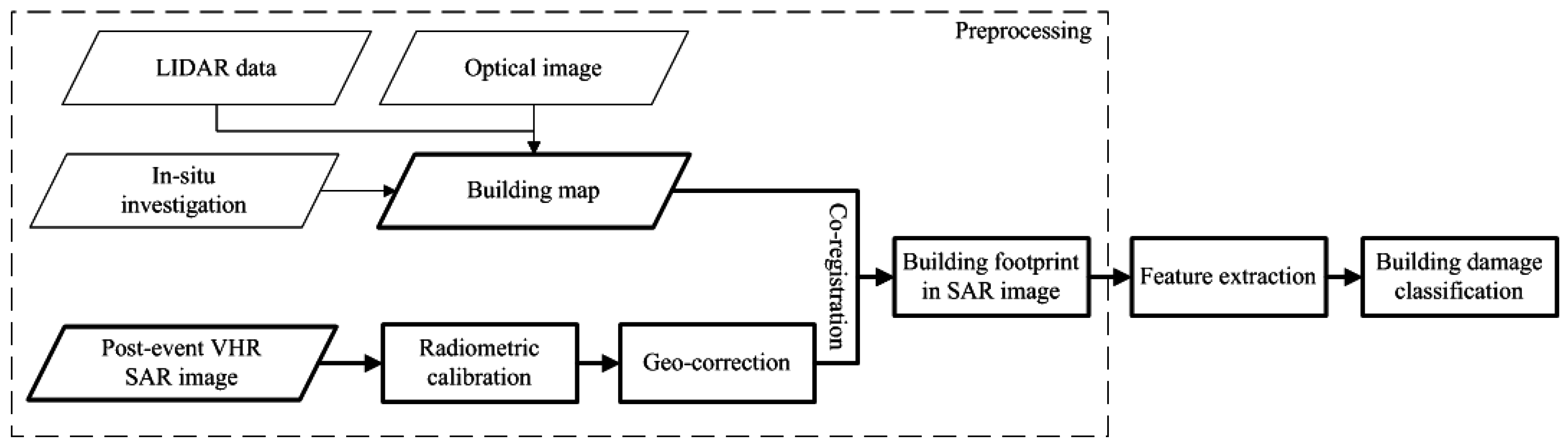The debris exhibits brighter scattering spots caused by smaller corner reflectors resulting from the composition of different planes [4]. Therefore, if the footprint of a building can be obtained, standing buildings and collapsed buildings can be separated based on features derived from the original footprint of the building. Based on this concept, we proposed a new scheme for detecting totally destroyed buildings with post-event single polarization VHR SAR images (Figure 7).

3.2. Preprocessing

The main inputs of the method are a sub-meter resolution SAR image and a building footprint map. Before analysis, the digital numbers of the TerraSAR-X SAR data were converted into radar sigma naught values as follows [13]:

σ° = (k_s × |DN|² − NEBN) ×sinθ_loc

(1)

where k_s is the calibration and processor scaling factor given by the parameter calFactor in the annotated file, DN is the pixel intensity value and NEBN is the noise equivalent beta naught. It represents the influences of different noise contributions on the signal. θ_loc is the local incidence angle [13].

The building footprint map in Figure 7 can be provided by a cadastral map from the government. If there is no building footprint map of the affected area, the map can be obtained by interpreting high-resolution pre-earthquake optical images. Unfortunately, we have no pre-earthquake high-resolution remote sensing images covering the research area. Therefore, we obtained the building footprint map by careful interpretation of the post-earthquake optical image with information of the in situ investigation and LIDAR data of the research area in our experiment. To register the building footprint map, the SAR data should be geometrically rectified. The ground control points, which provide the relationships between pixel coordinates in the image and geo-coordinates, can be found in the XML file in SAR products. After geometric rectification, the SAR image can be matched to the building footprint map, which also has geo-coordinates information. To improve the registration precision, registration between the geo-rectified SAR images and optical image is implemented with ENVI software by manually selecting the control points in the images in our experiment. The SAR images we used are single look complex (SLC) products. For real operation, the geocoded ellipsoid corrected (GEC) or enhanced ellipsoid corrected (EEC) products of the SAR data can be ordered to avoid geometric rectification by users. Although a layover, shadow area of a building usually occurs in the very high resolution SAR image, the footprint indicates the real location of the building. Therefore, with the building footprint map, the original footprints of buildings can be located in the descending and ascending SAR images. Then, features can be extracted based on the footprints in the SAR image.

3.3. Features for Classification

Four first-order statistics and eight second-order image statistical measures are investigated for analysis and damage type classification.

3.3.1. First-Order Statistics

Statistical features including mean, variance, skewness and kurtosis are selected for first-order statistical analysis. Setting $f_1=\mu$ as the mean value and $f_2={\sigma }^2$ as the variance value, the skewness and kurtosis can be expressed as follows.

(1) Skewness:

$$f_3=\frac{E{\left(x-\mu \right)}^3}{{\sigma }^3}$$

(2)

In Equation (2), E($·$) represents the expected value of variables. Skewness is a measure of the asymmetry of the data distribution around the sample mean. If skewness is negative, the data are spread out more to the left of the mean than to the right. If skewness is positive, the data are spread out more to the right. The skewness of the normal distribution is zero [14].

(2) Kurtosis:

$$f_4= \frac{E{\left(x-\mu \right)}^4}{{\sigma }^4}$$

(3)

Kurtosis describes how peaked or flat a distribution is, with reference to the normal distribution. The kurtosis of the normal distribution is 3. If kurtosis has a high value, then it represents a sharp peak distribution in the intensity values about the mean and has a longer, fat tail. If kurtosis has a low value, it represents a flat distribution of intensity values with a short, thin tail [15].

Skewness and kurtosis are features that describe the position and shape of a data distribution. SAR data usually exhibit long-tail distributions, and standing and collapsed buildings show different pixel intensities based on the above analysis. Therefore, skewness and kurtosis are selected as features to describe these differences.

3.3.2. Second-Order Image Statistics

The second-order image statistics measure the relationships between pixels and their neighbors [16]. To calculate the second order statistics, the pixel values for a given scale of interest are first translated into a gray level co-occurrence matrix (GLCM). Texture measures derived from the GLCM have been widely used for land cover classification and other applications with radar and optical data.

GLCM describes the frequency of one gray tone appearing in a specified spatial linear relationship with another gray tone in the area under investigation [17]. The textural statistics are calculated based on GLCM. The GLCM-based textural features are second-order features widely used in texture analysis and image classification. Recently, GLCM features have been used to analyze the signatures of damaged buildings in real and simulated VHR SAR images [8,10,18].

Haralick et al. proposed 14 features based on GLCM for textural analysis [19]. These features measure different aspects of the GLCM, and some features are correlated. In this paper, eight texture features are chosen for analysis: the mean, variance, homogeneity, contrast, dissimilarity, entropy, second moment and correlation. Let $p\left(i,j\right)$ be the $\left(i,j\right)$-th entry in a normalized GLCM. The features are as follows [19,20,21].

(1)

Mean:

$$g_1={\displaystyle \sum }_i{\displaystyle \sum }_{j}i\times \left(i,j\right)$$

(4)

(2)

Variance:

$$g_2={\displaystyle \sum }_i{\displaystyle \sum }_j{\left(i-\mu \right)}^{2}p\left(i,j\right)$$

(5)

(3)

Homogeneity:

$$g_3={\displaystyle \sum }_i{\displaystyle \sum }_j\frac{1}{1+{\left(i-j\right)}^2}p\left(i,j\right)$$

(6)

(4)

Contrast:

$$g_4= {\displaystyle \sum }_{n=0}^{N_g-1}{n}^2\left\{{\displaystyle \sum }_{i=1}^{N_g}{\displaystyle \sum }_{j=1}^{N_g}p\left(i,j\right)|\left|i-j\right|=n\right\}$$

(7)

In Equation (7), $N_g$ is the number of distinct gray levels in the quantized image.

(5)

Dissimilarity:

$$g_5={\displaystyle \sum }_i{\displaystyle \sum }_j\left|i-j\right|\times p\left(i,j\right)$$

(8)

(6)

Entropy:

$$g_6= -{\displaystyle \sum }_i{\displaystyle \sum }_{j}p\left(i,j\right)\log \left(p\left(i,j\right)\right)$$

(9)

(7)

Second moment:

$$g_7= {\displaystyle \sum }_i{\displaystyle \sum }_j{\left\{p\left(i,j\right)\right\}}^2$$

(10)

(8)

Correlation:

$$g_8=\frac{{{\displaystyle \sum }}_i{{\displaystyle \sum }}_j\left(ij\right)p\left(i,j\right)-{\mu }_x{\mu }_y}{{\sigma }_x{\sigma }_y}$$

(11)

where ${\mu }_{x,}{\mu }_y, {\sigma }_x$ and ${\sigma }_y$ are the means and standard deviations of $p_x$ and $p_y$.

The GLCM mean measures the average gray level in the GLCM window. The GLCM variance measures the gray level variance and is a measure of heterogeneity. GLCM homogeneity, which is also called the inverse difference moment, measures the image homogeneity, assuming larger values for smaller gray tone differences in pair elements. GLCM contrast is a measure of the amount of local variation in pixel values among neighboring pixels. It is the opposite of homogeneity. GLCM contrast is related to first-order statistical contrast. Thus, high contrast values reflect highly contrasting textures. GLCM dissimilarity is similar to contrast and inversely related to homogeneity. GLCM entropy measures the disorder in an image. When the image is not texturally uniform, the value will be very large. The GLCM second moment is also called energy. It measures textural uniformity. If the image patch is homogeneous, the value of the second moment will be close to its maximum, which is equal to 1. GLCM correlation is a measure of the linear dependency of pixel values on those of neighboring pixels. A high correlation value (close to 1) suggests a linear relationship between the gray levels of pixel pairs. Therefore, we can see that the GLCM homogeneity and second moment are measures of homogenous pixel values across an image, while the GLCM contrast, dissimilarity and variance are measures of heterogeneous pixel values. Based on the analysis of Section 2, we can observe that the standing building shows relative homogeneity in the footprint, while the collapsed building shows more heterogeneity. Therefore, these features are selected for analysis. In addition, the GLCM mean, entropy and correlation are also considered for analysis. In this paper, image texture measures are calculated for every pixel using ENVI software.

3.4. Classifier

Three machine learning methods involving random forest (RF) [22], support vector machine (SVM) [23] and K-nearest neighbor (K-NN) [24] classifiers are used to classify collapsed and standing buildings in our experiments.

Ensemble learning algorithms (e.g., random forest) have received increased interest because they more accurately and robustly filter noise compared to single classifiers [22,25,26]. RF is an ensemble of classification trees, where each tree contributes a single vote to the assignment of the most frequent class of the input data. An RF can handle a number of input variables without variable deletion, and it estimates the importance of variables in the classification.

Support vector machine (SVM) is a supervised learning model with associated learning algorithms that analyze data and recognize patterns based on the structural risk minimization principle in statistics.

The K-NN algorithm is a statistical instance-based learning method [27,28]. It decides that a certain pattern X belongs to the same category as its closest neighbors given a training set of m labeled patterns. The algorithm estimates the probabilities of the classes using a Euclidian metric.

The three machine learning methods are supervised classifiers, and they have been widely used for remote sensing image classification. We adopt the methods to evaluate the results of building damage detection using VHR SAR images.

4. Study Area and Materials

The study area is located in old Beichuan County. On 12 May 2008, the Wenchuan Earthquake with a magnitude of 8.0 occurred in Sichuan province, China [29]. The earthquake devastated a huge area in Sichuan province, killing and injuring a large number of people and causing major damage to buildings and other infrastructures. Beichuan County (centered at approximately 31.833°N and 104.459°E) was one of the most affected areas. The Beichuan County was originally located in Qushan Town. After the earthquake, the county was moved to Yongchang Town, which belonged to An County before the earthquake. The old Beichuan County seat was abandoned, and some ruins were preserved as the Beichuan Earthquake Memorial Park. The study area belongs to the Beichuan Earthquake Memorial Park. Therefore, some damaged buildings are preserved in the area and can be selected for analysis.

Three decimeter level resolution TerraSAR-X ST mode SAR images acquired in 2014 and 2015 are used for analysis and experimentation. One is ascending SAR image, and two are descending SAR images. TerraSAR-X ST SAR is a new mode that was introduced in 2013 by the German Aerospace Center (DLR). With the new mode, a spatial resolution of approximately 0.24 m can be achieved in the azimuth direction of the system by widening the azimuth beam steering angle range [30]. With coarse spatial resolution data, damage detection is usually performed on the building group or residential area level. While in the VHR SAR image, much more building features like edges and point structures become visible. Therefore, it is possible to focus an analysis on individual buildings.

Table 1. Detailed image information.

Number	Polarization	Orbit Direction	Date of Acquisition	Resolution (m)		Look Direction	Incidence Angle (°)
				Ground Range	Azimuth
1	HH	Ascending	4 December 2014	0.86	0.23	Right	43.0
2	HH	Descending	8 December 2014	0.86	0.23	Right	42.6
3	HH	Descending	8 April 2015	0.86	0.23	Right	42.8

gives detailed information regarding the data.

An optical multispectral image and LIDAR data covering the study area are used as reference data. In May 2013, 5 years after the earthquake, the Airborne Remote Sensing Center (ARSC) of the Institute of Remote Sensing and Digital Earth carried out a campaign for monitoring the areas affected by the Wenchuan earthquake in 2008. One remote sensing airplane carrying an optical ADS80 sensor collected a number of images of the areas, including the old Beichuan County. The data acquired by ADS80 are multi-spectral images, and the resolution of the image is approximately 0.6 m. The optical image has been rectified when we obtained it from ARSC. In situ investigations were carried out in 2014 and 2015, corresponding to the ST SAR data acquisition dates. Based on the post-earthquake optical image, LIDAR data and in situ investigation, a reference map of the standing and collapsed buildings can be generated by careful interpretation. The reference map of the standing and collapsed building can be regarded as the ground truth for analysis and validation. 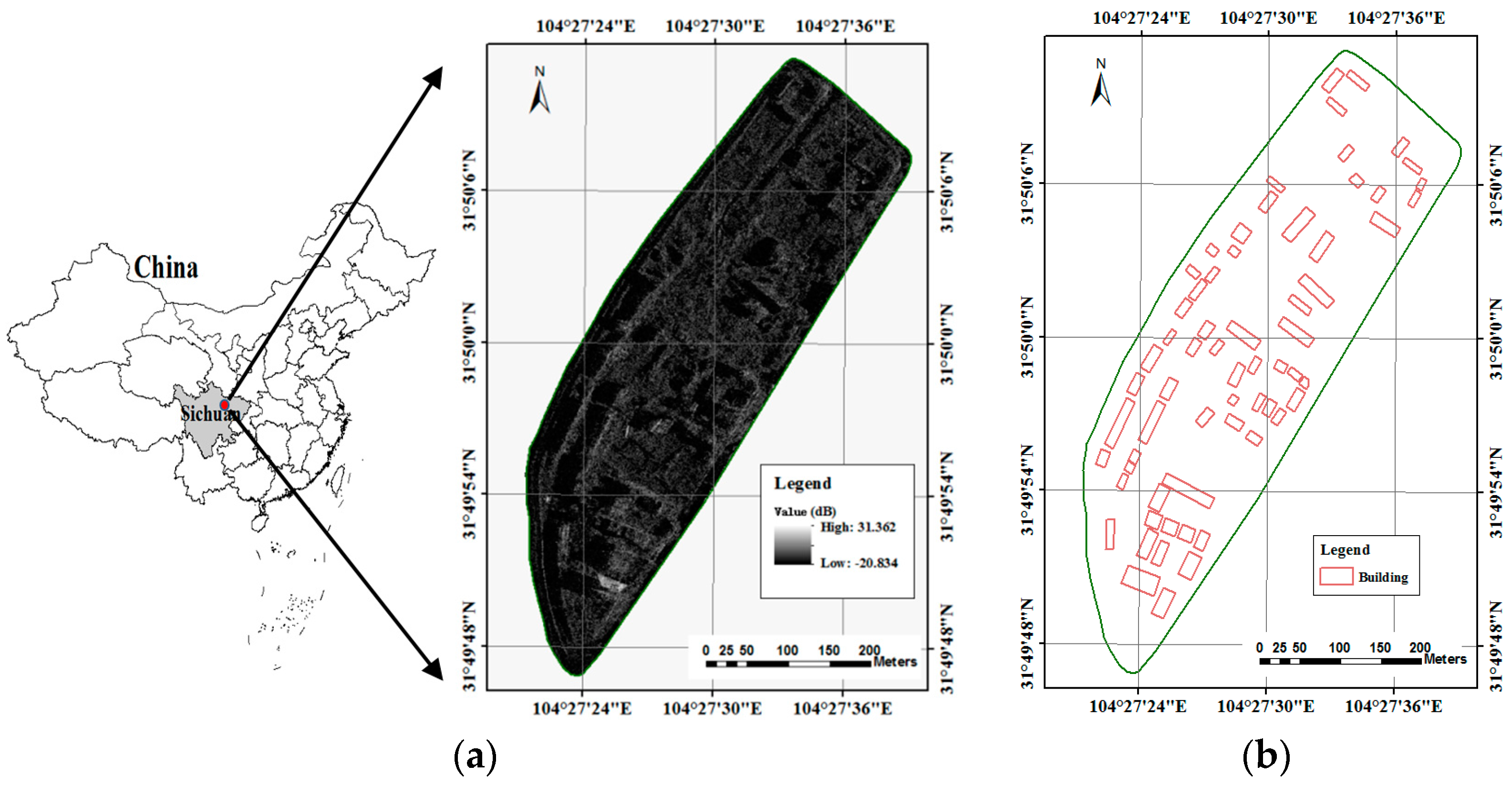Figure 8 illustrates the research area, the SAR image and building footprint map. 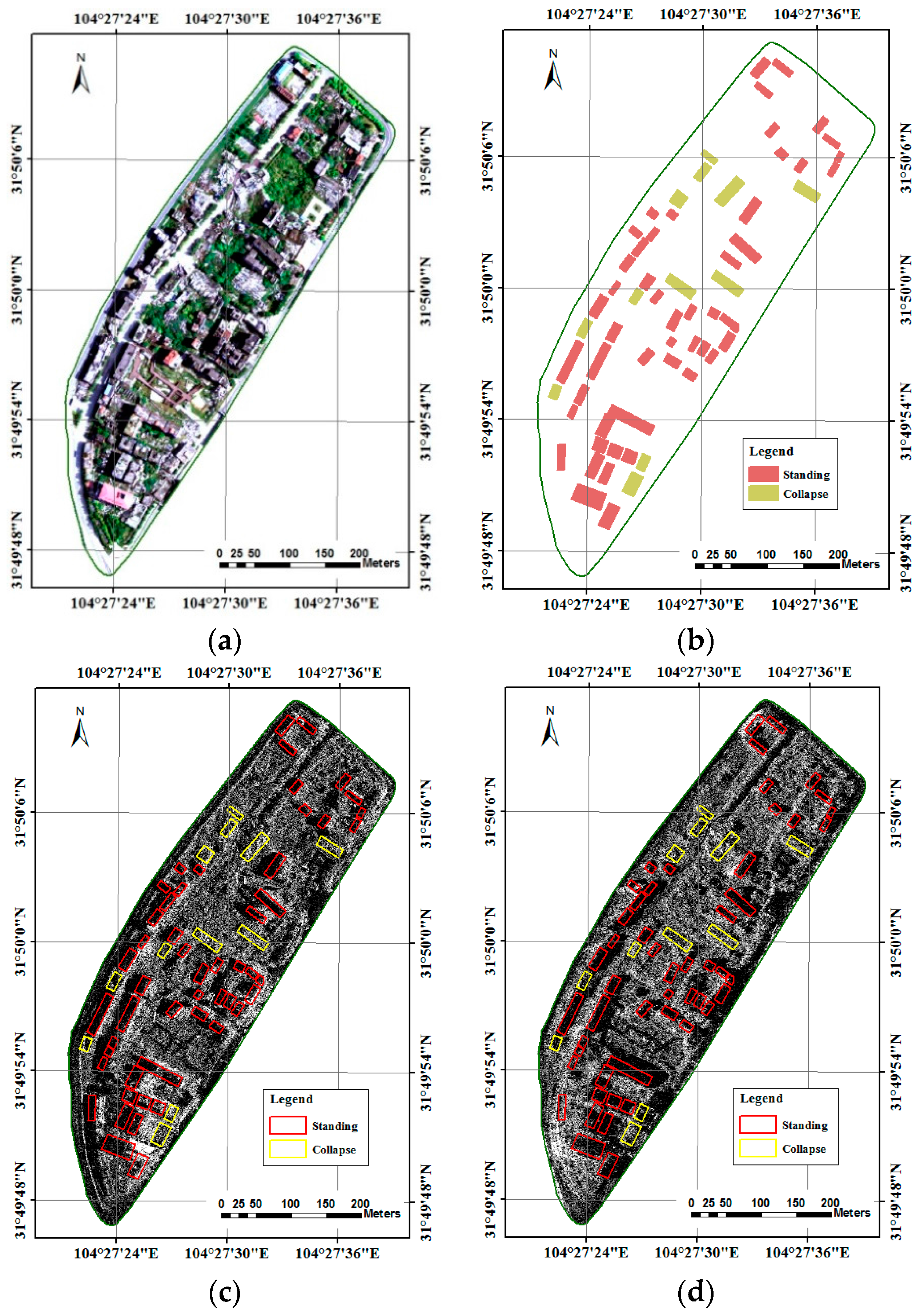Figure 9 presents the optical image (Figure 9a) and the reference map (Figure 9b). Figure 9c,d illustrates a descending and ascending SAR image superimposed by the reference map, respectively. In order to illustrate the image more clearly, the values of the SAR image in Figure 9c,d have been stretched to the 0–255 gray level. The building footprint map and reference map are generated by optical image, LIDAR data and in situ investigations.

5. Experimental Results and Analysis

Three sub-meter VHR TerraSAR-X ST SAR images are used in the experiments and algorithm evaluation. With the building footprint map, the original footprints of the buildings can be obtained in the SAR images. Then, the features are calculated, forming a feature vector $FV=\left\{f_1,f_2,f_3,f_4,g_1,g_2,g_3,g_4,g_5,g_{6,}{g}_7,g_8\right\}$ for classification.

5.1. Parameters of GLCM-Based Textural Features

Generally, if the textural measures derived from the GLCM are used, some fundamental parameters should be defined, including the quantization levels of the image, the window size used to calculate the GLCM and the displacement and orientation values of the measurements.

5.1.1. Quantization Level

The quantization level is a fundamental parameter. A value that is too low can lead to substantial information reduction. However, fewer levels reduce noise-induced effects and directly affect the computing cost because the number of bins determines the size of the co-occurrence matrix [7]. This tradeoff was discussed by Soh et al. [20], with the conclusion that 64 levels are suggested for sea ice in SAR images. Additionally, they have that a 256-level representation is not necessary and an eight-level representation is undesirable. A level of 256 was applied in [16]; a level of 128 was adopted in [7]; and a 64-level quantization was applied in [8] to detect and distinguish debris in SAR images. Additionally, 16-level, 64-level and 32-level quantization was adopted in [31,32,33], respectively, for sea ice classification and other applications. Based on [20] and [7,8], a 64-level quantization using ENVI software is adopted in our experiments. 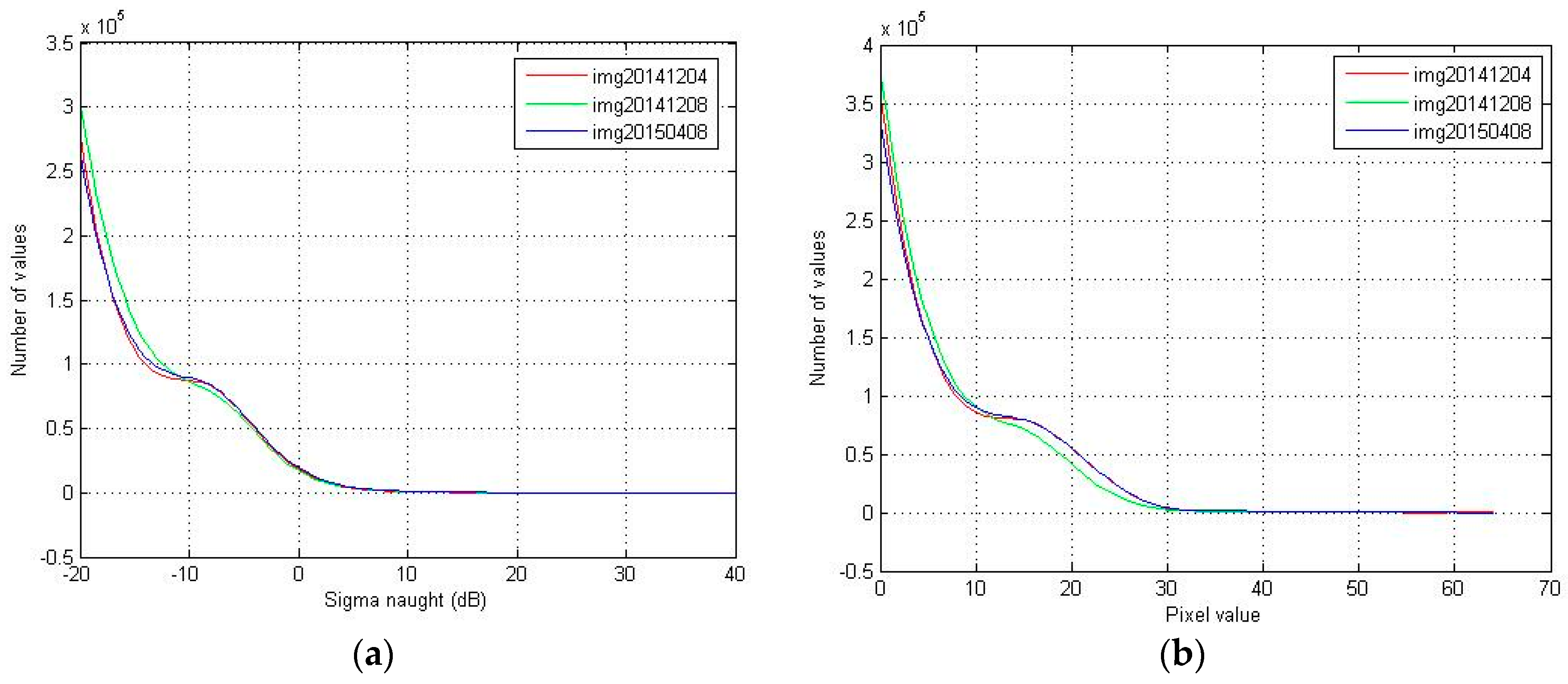Figure 10 illustrates the histograms of the sigma naught of the SAR images (Figure 10a) and the 64-level quantization images by ENVI (Figure 10b). It shows that the shapes of the histograms of the images are kept well after quantization.

5.1.2. Window Size

In order to calculate texture features for each pixel in an image, a moving window is usually used to define the neighborhood of a pixel, and the texture measurement calculated from the window is assigned to the center pixel [26,34]. The window size for texture analysis is usually related to image resolution and the contents within the image. However, it might be difficult to determine the window size through a formula. In the experiments, we chose 13 × 13 pixels as the window size to calculate the texture features. The analysis is as follows.

(1) Estimation by classification result:

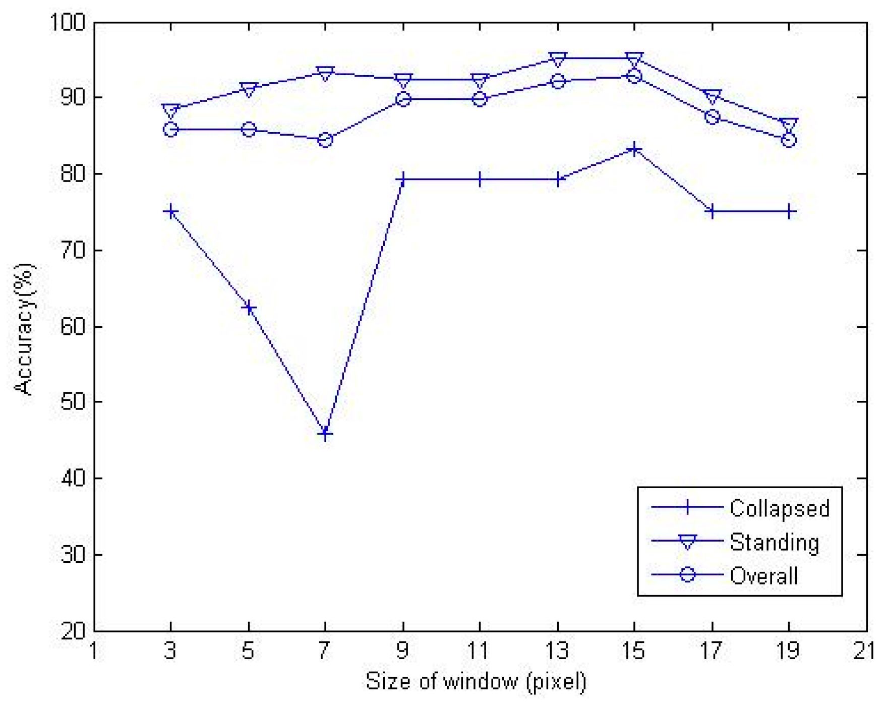
The overall accuracy or kappa coefficient of the classification results is usually applied for estimating the window size [26,34]. If the texture features can give the highest classification accuracy, then the widow size will be chosen as the optimal size. Figure 11 shows the influence of window size on the overall accuracy and accuracy of the classification results of texture features for collapsed and standing buildings. The classifier is random forest. With the whole of 192 samples (36 collapsed buildings, 156 standing buildings), 1/3 of samples are for training, and 2/3 of samples are for testing. The figure shows that the classification results of small window size are not stable. The overall accuracy increases when the window size is larger than 7 × 7 pixels and decreases when the window size is larger than 15 × 15 pixels. The overall accuracy is stable when the window size is between 9 × 9 pixels and 15 × 15 pixels. It appears that the window sizes of 13 × 13 pixels and 15 × 15 pixels can be identified as appropriate to achieve best overall accuracy.

(2) Estimation by coefficient of variation of texture measures:

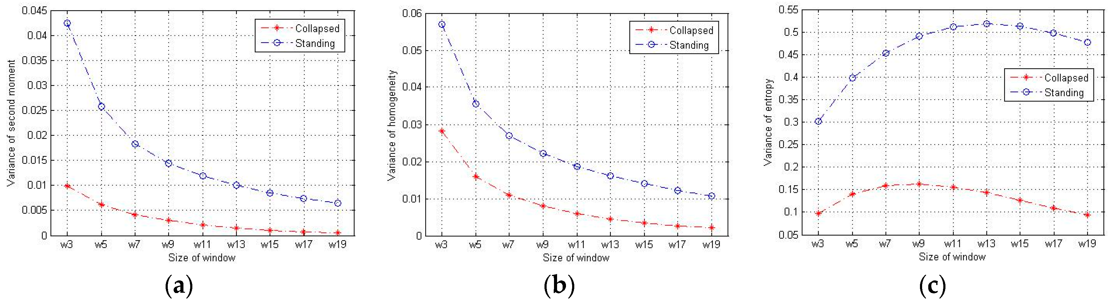
To facilitate the choice of an optimal texture window, the coefficient of variation of each texture measure for each class in relation to window size was also calculated [35]. The chosen optimal window size is usually that in which the value of the coefficient of variation starts to stabilize to the smallest value [35]. Figure 12 presents the evolution of the variance in relation to different window sizes for the textural measures. Figure 12a–c is the results of the second moment, homogeneity and entropy, respectively. The red starred line indicates the collapsed building, and the blue open-circled line represents the standing building values. The variances of textural features of the second moment and homogeneity decrease at larger window sizes; while the values of entropy show general increasing trends at small window sizes and decrease with increasing window size. The variation starts to stabilize at a 13 × 13 pixels window in Figure 12a–c. The results show that a 13 × 13 pixels window size can be a good choice for the textural measures.

(3) Estimation by visual interpretation:

If the building is still standing, the footprint is usually covered by shadow area. If the building is collapsed, the footprint is usually covered by debris. Figure 13 shows examples of shadow and debris in building footprints in the SAR image. The red and yellow rectangles indicate the footprints of standing and collapsed buildings, respectively. The debris usually contains some heaps of randomly-oriented planes mainly made of concrete. The planes are usually not very large and may be 1–3 m in width or length. After geometric rectification, the SAR image is resampled to a 0.6-pixel spacing, which is the same as the optical image. Therefore, in the 0.6-pixel spacing SAR image, the planes may be usually 2–5 pixels (Figure 13). Consequently, we think the window size of 13 × 13 pixels may be proper for texture analysis.

Generally, the larger the window size is, the coarser the information that can be provided by textural features. Therefore, the window size used to compute textural features should not be too large. Based on the quantitative and qualitative analysis, a 13 × 13 pixels window size is chosen to calculate the GLCMs in the experiments.

5.1.3. Orientation and Displacement

The orientation parameter is less important compared to other factors in the co-occurrence matrix [20]. We investigate the values of the textural measures of collapsed (red starred line) and standing buildings (blue open-circled line) in four directions, including 0°, 45°, 90° and 135°. Figure 14 gives the results of the values of GLCM-based textural features with different orientations. It shows that the features have relatively stable values when the orientation changes. However, we also found that the texture features of 45° and 135° have similar values. Additionally, they have some differences from the values in 0° and 90°. In Figure 9, it can be observed that most of the buildings’ orientations are about 135° or 45°. This may be the reason that the values of features in 45° and 135° have a similar tendency. In the experiments, the orientation of 135° is chosen for the calculation of GLCM.

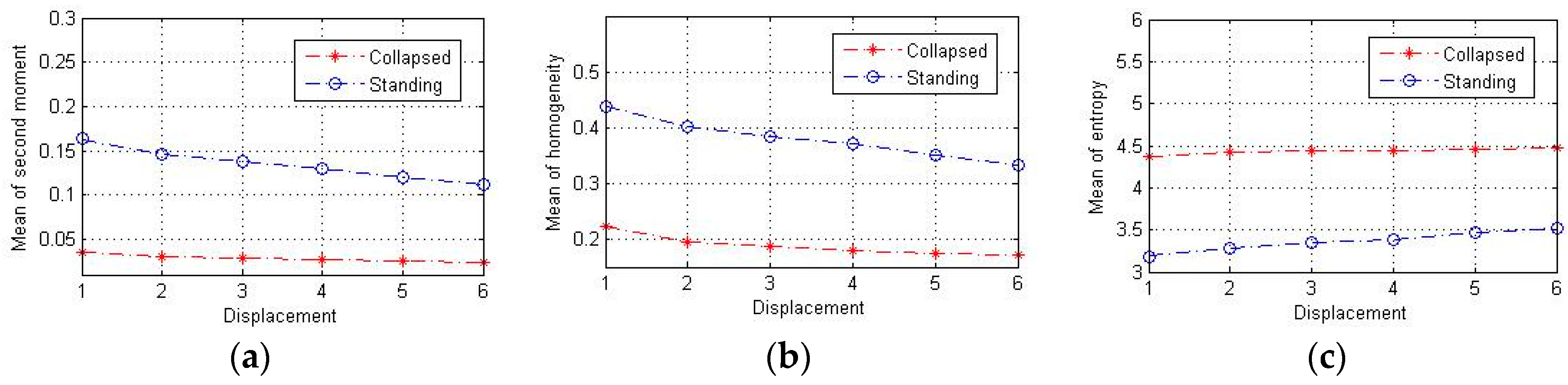
The GLCM describes the probability of finding two given pixel gray-level values in a defined relative position in an image [36]. Displacement indicates the inter-pixel distance. Figure 15 presents the investigation of GLCM features with different displacements. In the experiment, the features are calculated at an orientation of 135°, with a 13 × 13 window size. The results show that the values changed little when the displacement increased, indicating that the parameter displacement is not important in the co-occurrence matrix. The ideal distance of pixel offset depends on the level of detail of the texture that is analyzed. The GLCM cannot capture fine-scale textual information if a large pixel offset is used [7]. Accordingly, in our experiment, an orientation of 135° and a displacement of one are selected.

5.2. Classification Results

5.2.1. Features for Classification

Classification experiments had been carried out for features analysis. Random forest (RF) is the classifier. Based on the reference map, we obtained original footprints of 12 totally collapsed buildings and 52 standing buildings (Figure 9b) in each image. For each test, 6 collapsed buildings and 17 standing buildings are used to train samples, and the corresponding numbers of test samples are six and 35, respectively.

Table 2. Classification results with only first-order statistics (CO = totally collapsed building, ST = standing building; Pa = producer’s accuracy, Ua = user’s accuracy).

Type	Classification
	8 April 2015			4 December 2014			8 December 2014
	CO	ST	Pa	CO	ST	Pa	CO	ST	Pa
CO	5	1	83.3%	4	2	66.7%	6	0	100%
ST	6	29	82.8%	6	29	82.8%	3	32	91.4%
Ua	45.5%	96.7%		40%	93.5%		66.7%	100%
Overall	82.9%			80.5%			92.7%

shows the classification results with only first-order statistics.

Table 3. Classification results with only second-order statistics (CO = totally collapsed building, ST = standing building; Pa = producer’s accuracy, Ua = user’s accuracy).

Type	Classification
	8 April 2015			4 December 2014			8 December 2014
	CO	ST	Pa	CO	ST	Pa	CO	ST	Pa
CO	5	1	83.3%	5	1	83.3%	5	1	83.3%
ST	3	32	91.4%	5	30	85.7%	6	29	82.9%
Ua	62.5%	97.0%		50%	96.8%		45.5%	96.7%
Overall	90.2%			85.4%			82.9%

is the classification results with only second-order statistics.

Table 4. Classification results with all features (CO = totally collapsed building, ST = standing building; Pa = producer’s accuracy, Ua = user’s accuracy).

Type	Classification
	8 April 2015			4 December 2014			8 December 2014
	CO	ST	Pa	CO	ST	Pa	CO	ST	Pa
CO	6	0	100%	5	1	83.3%	6	0	100%
ST	5	30	85.7%	3	32	91.4%	4	31	88.6%
Ua	54.5%	100%		62.5%	97.0%		60%	100%
Overall	87.8%			90.2%			90.2%

gives the classification results with all features.

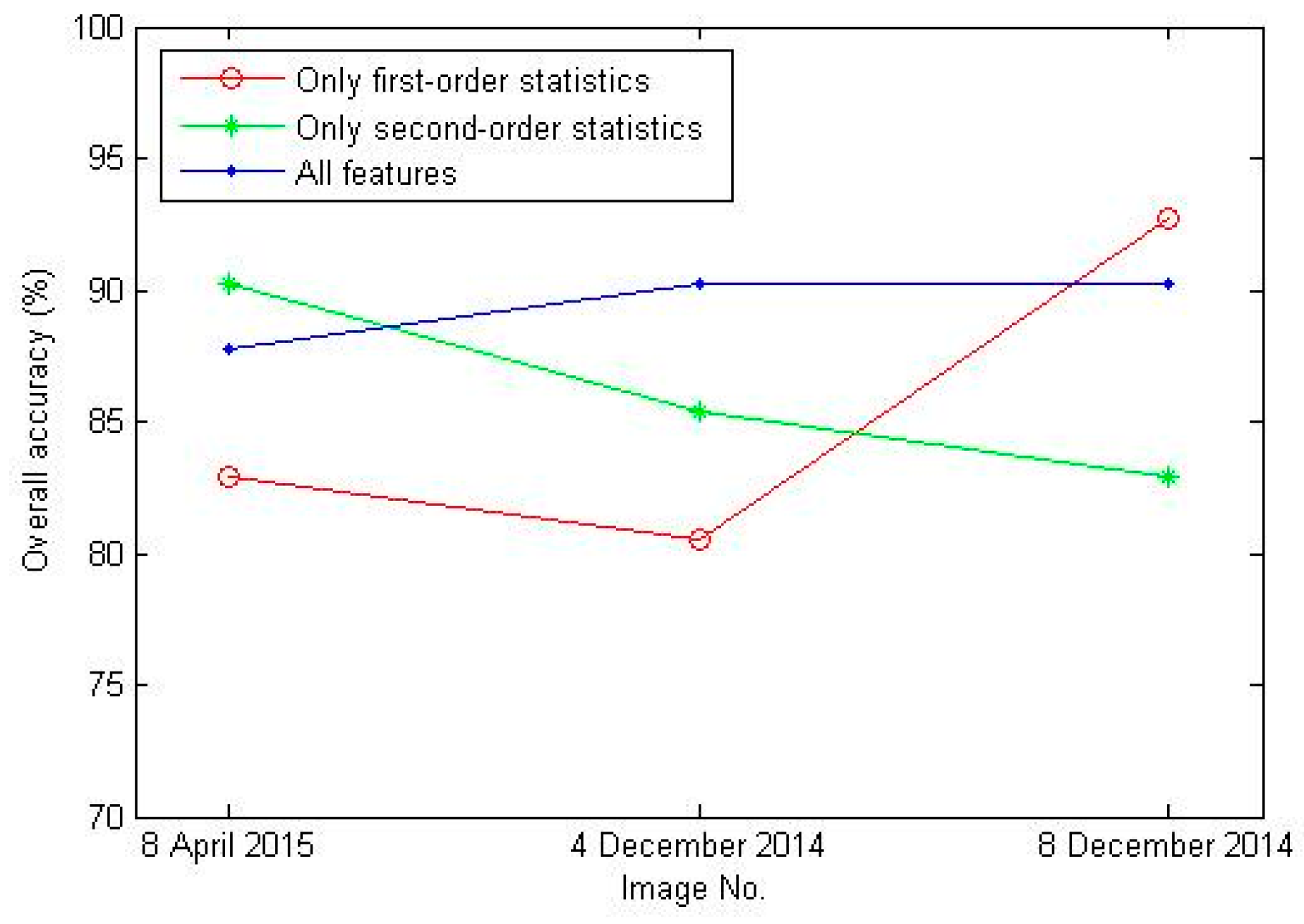
Figure 16 illustrates the overall accuracy of the classification results of different images with different features. The red line in Figure 16 is the results with only first-order statistics of the images. The green line indicates the results with only second-order statistics of the images. The blue line is the results with all features of the images. It shows that the classification result with all features is good and stable for all images, and the overall accuracies are all above 85%. However, the results are relatively unstable with only first-order statistics and only second-order statistics. As mentioned in Section 3.3, the mean and variance values can describe the difference of backscattering of the standing and collapsed buildings. The skewness and kurtosis reflect the difference of shapes of histograms of the standing and collapsed buildings. The textural measures can reveal textural characteristics of the two kinds of buildings. Therefore, all features are recommended for classification due to the good ability to discriminate the standing and collapsed buildings.

5.2.2. Classification Results

Based on the reference map, we obtained original footprints of 12 totally collapsed buildings and 52 standing buildings (Figure 8b) in each image. For each classifier, six collapsed buildings and 17 standing buildings are used to train samples, and the corresponding numbers of test samples are six and 35, respectively. In the experiments, 10, 20, 50, 100 and 200 trees are used for the RF classifier, and the classification result with the highest accuracy is recorded and reported. For the SVM classifier, the C-support vector classification (C-SVC), which was introduced by Cortes et al. [37] and presented by Chang and Lin [23], is adopted. As suggested by Chang, the radial basis function (RBF) is chosen as the kernel function to construct the classifier. Furthermore, the two parameters (the kernel width and penalty coefficient) of the RBF are determined by performing a grid search and cross-validation method in our study.

Table 5. Classification results of Image 1 using different methods (CO = totally collapsed building, ST = standing building; Pa = producer’s accuracy, Ua = user’s accuracy).

Type	Classification
	RF			SVM			K-NN
	CO	ST	Pa	CO	ST	Pa	CO	ST	Pa
CO	5	1	83.3%	6	0	100%	6	0	100%
ST	3	32	91.4%	4	31	88.6%	9	26	74.3%
Ua	62.5%	97.0%		60%	100%		40%	100%
Overall	90.2%			90.2%			80.5%

,

Table 6. Classification results of Image 2 using different methods (CO = totally collapsed building, ST = standing building; Pa = producer’s accuracy, Ua = user’s accuracy).

Type	Classification
	RF			SVM			K-NN
	CO	ST	Pa	CO	ST	Pa	CO	ST	Pa
CO	6	0	100%	6	0	100%	6	0	100%
ST	4	31	88.6%	4	31	88.6%	5	30	85.7%
Ua	60%	100%		60%	100%		54.5%	100%
Overall	90.2%			90.2%			87.8%

and

Table 7. Classification results of Image 3 using different methods (CO = totally collapsed building, ST = standing building; Pa = producer’s accuracy, Ua = user’s accuracy).

Type	Classification
	RF			SVM			K-NN
	CO	ST	Pa	CO	ST	Pa	CO	ST	Pa
CO	6	0	100%	6	0	100%	6	0	100%
ST	5	30	85.7%	3	32	91.4%	7	28	80%
Ua	54.5%	100%		66.7%	100%		46.2%	100%
Overall	87.8%			92.7%			82.9%

present the classification results of different classifiers in the three images. For Image 1, Table 5 shows that the collapsed buildings can be classified well by the three classifiers. Only one collapsed building was misclassified as a standing building by the RF. The K-NN classifier gives the lowest overall accuracy of 80.5%, as there are six standing buildings misclassified as collapsed buildings. The overall accuracies of RF and SVM reach 90.2%. For Image 2, Table 6 shows that RF and SVM yield the same results, with overall accuracies of 90.2%. The overall accuracy of K-NN is 87.8%. For Image 3, Table 7 shows that SVM gives the best result, with an overall accuracy of 92.7%. The overall accuracies of RF and K-NN are 87.8% and 82.9%, respectively.

Based on the analysis above, collapsed buildings and standing buildings can be effectively separated by the three classifiers, as the overall accuracies of the three classifiers all exceed 80%. The results of RF and SVM are similar, and these methods outperform the K-NN classifier. Thus, collapsed buildings can be detected well by the proposed method.

5.2.3. Further Analysis about the Classification

In our experiments, the classifiers adopted are supervised classifiers. Furthermore, they are also machine learning techniques. The training dataset is very important for these classifiers. To obtain the training samples, the ground truth must be known. However, after the training dataset has been built, the classifier can be performed when a new SAR image is input.

Table 8. RF classification results of different tests (CO = totally collapsed building, ST = standing building, Pa = producer’s accuracy, Ua = user’s accuracy. In Test 1 and Test 2, the training dataset is samples from Image 3 (8 April 2015) and Image 2 (8 December 2014), respectively. In Test 3, the training dataset is all samples from Images 2 and 3. Image 1 (4 December2014) is the input for classification of all of the tests).

Type	Classification
	Test 1			Test 2			Test 3
	CO	ST	Pa	CO	ST	Pa	CO	ST	Pa
CO	6	6	50.0%	8	4	66.7%	8	4	66.7%
ST	1	51	98.1%	4	48	92.3%	3	49	94.2%
Ua	85.7%	89.5%		66.7%	92.3%		72.7%	92.5%
Overall	89.1%			87.5%			89.1%

shows the results of three tests by the RF classifier. The aim of the tests is to evaluate the ability to classify a new image based on an existing training dataset. In Test 1 and Test 2, the training dataset is samples from Image 3 (8 April 2015) and Image 2 (8 December 2014), respectively. In Test 3, the training dataset is all samples from Images 2 and 3. Image 1 (4 December 2014) is the input image for the classification of all of the tests. As mentioned in Table 1, Images 2 and 3 are descending images, and Image 1 is an ascending image. In Test 1, the accuracy of the collapsed building is not good. However, the result of Test 2 is acceptable. In Test 3, the results are stable and improved slightly. The results indicate that it is possible to classify a new image if there is an existing training dataset for the classifier. The result will be better if the training dataset contains more training samples. In future work, more samples should be acquired, and images of other research sites should be tested for a more precise conclusion.

6. Discussion

Compared with low- or medium-resolution SAR images, VHR SAR image can provide more detailed information of man-made objects, such as buildings. In 2013, the TerraSAR-X mission was extended by implementing two new modes including the staring spotlight. The azimuth resolution of this mode is significantly increased to approximately 0.24 m by widening the azimuth beam steering angle range [30]. The sub-meter VHR SAR data source provides new opportunities for earthquake damage mapping and makes it possible to focus an analysis on individual buildings. A new method is proposed in the paper to use these VHR SAR data for collapsed building detection. The method is based on the concept that the original footprints of collapsed and standing buildings show different features in sub-meter VHR SAR images. In an SAR image, the shadow of a standing building covers the majority of the building’s footprint; thus, the footprint of a standing building usually exhibits low backscattering intensity. For a collapsed building, debris piles up above the footprint. Some bright spots can be observed, which are caused by corner reflectors resulting from the composition of different planes. Therefore, the collapsed building displays different features than do standing buildings in their original footprints. For the proposed method, the features for classification are derived from building footprints. Therefore, the high image resolution is the key factor to ensure that the building footprint contains more pixels for classification. If the building size is large, it also will benefit building damage detection.

The proposed method avoids the difficulties of finding exact edges for building damage detection. In VHR SAR images, more features, such as the points and edges of objects, become visible. Debris exhibits similar features as the surroundings (e.g., vegetation). It is not easy to identify debris from surroundings such as vegetation with a single SAR image. To solve this problem, the proposed method uses a building footprint map to locate the original footprints of buildings. The key algorithm begins with the footprint of a building in an SAR image. The footprint of a building can be provided by cadastral maps or directly extracted from a pre-event SAR image or other VHR optical data.

The approach shows a good ability for isolated buildings. However, if the buildings are too close, the footprint of a low building may be affected by a nearby tall building’s layover in the image. Because the layover usually shows relatively high backscattering intensity, the low standing building may be misclassified as a collapsed building by the method. If the debris of a collapsed building is near a standing building, the incidence wave from the senor may be obstructed by the standing building, as little of the backscatter wave from the collapsed building can be received by the sensor. In this case, the collapsed building also shows low backscattering intensity in the footprint, and it may be misclassified as a standing building.

The high resolution of an SAR image usually means small coverage of a single scene. The scene extent of a TerraSAR-X ST mode image usually varies between 2.5 and 2.8 km in the azimuth direction and 4.6 km and 7.5 km in the range [30,38]. The small coverage of ST mode data may not be adequate for damage detection over a wide area with a single image. Commercial TerraSAR-X services commenced in January 2008. A TerraSAR-X rebuild was launched as TanDEM-X in 2010 to fly in close formation with TerraSAR-X [39]. The almost identical Spanish PAZ satellite will be launched in 2016 [40] and added to the TerraSAR-X reference orbit. The three almost identical satellites will be operated collectively and deliver optimized revisit times, increase coverages and improve services [41]. When we monitor Earth surface deformation by earthquakes, SAR images with large coverages are preferable. When detecting building damage in a town or a city, the coverage requirements of the image may be smaller. If the study area is a large city, the data can be acquired from TerraSAR-X , TanDEM-X and PAZ to cover a large area. Therefore, in real applications, we can use large-coverage SAR images to locate the city or town influenced by an earthquake and perform preliminary damage assessments. The ST data from TerraSAR-X , TanDEM-X and PAZ can be obtained to monitor the region for a more detailed and accurate assessment. In addition, airborne VHR SAR images covering the study area can be used to detect building damage.

7. Conclusions

In this paper, we present a new damage assessment method for buildings using single post-earthquake sub-meter resolution VHR SAR images and original building footprint maps. The method can work at the individual building level and determines whether a building is destroyed after an earthquake or is still standing. First, a building footprint map covering the study area is obtained as prior knowledge. Then, an SAR image is geometrically rectified by the ground control points provided by the SAR product files. After rectification, the SAR image can be registered as the building footprint map. Thus, with the building footprint map, the original footprint of a building can be located in the SAR image. Then, features can be extracted in the image patch of a building’s footprint to form a feature vector. Finally, the buildings can be classified into damage classes with classifiers.

We demonstrated the effectiveness of the proposed approach using spaceborne post-event sub-meter VHR TerraSAR-X ST mode data from old Beichuan County, China, which was heavily damaged in the Wenchuan earthquake in May 2008. The results show that the method is able to distinguish between collapsed and standing buildings, with high overall accuracies of approximately 90% for the RF and SVM classifiers. We tested the method using both ascending and descending data, demonstrating the effectiveness of the proposed method. The results also show that the first-order statistics and second-order image features derived from building footprints have a good ability to discriminate standing and collapsed buildings. Furthermore, for the supervised classifiers in our experiments, after the training dataset has been built, the classifier can be well performed when a new SAR image is input. In future work, more samples should be acquired, and images of other research sites should be tested for a more precise conclusion.