1. Introduction
Hyperspectral sensors have become a key tool for a large range of applications in remote sensing and are now widely used in geology, mineral mapping and exploration (e.g., van der Meer et al. [
1], Laakso et al. [
2], Jakob et al. [
3], Zimmermann et al. [
4]). During the last few years, lightweight hyperspectral imaging (HSI) sensors have been increasingly developed for use on unmanned aerial systems (UAS) (i.e., Cubert GmbH [
5] or Rikola Ltd. [
6]). These drone-borne sensors are able to close the gap between field- and air- or space-borne data and provide small-scale high-resolution hyperspectral imagery (Watts et al. [
7]). The acquisition of image data with UAS is fast, easy, targeted and without the need of extensive time- and cost-consuming planning. It is mostly independent of cloud cover conditions and is even applicable in barely accessible areas. The heavily decreased influence of the atmosphere obviates the need for the often difficult and complex atmospheric correction. Nevertheless, geometric and radiometric correction of drone-borne data is challenging mainly due to small, unpredictable platform shifts and the influence of the micro-topography. Thus, high resolution digital elevation models are required for correction. Common and established workflows for the pre-processing of aerial hyperspectral scanner data (e.g., Schläpfer and Richter [
8], Richter and Schläpfer [
9]) are not or only partly applicable.
Sensors in the visible and near-infrared spectral range (VNIR) of the electromagnetic spectrum have been preferably used on UAS due to their low weight and size. In contrast, short wave infrared (SWIR) sensors exceed the payload capacity of most lightweight aerial platforms. Larger UAS with higher payload complicate the handling in remote areas and increase the difficulty to obtain flight permission by the local authorities in most countries.
The most prominent material absorption features in the VNIR spectral range originate from green vegetation, while only a few mineral groups, mainly iron oxides and some rare earth elements, show typical absorption features. Those mineralogical features can be quite shallow, and their truthful determination depends mainly on an accurate data correction. By contrast, the occurrence and health analysis of vegetation is easily determinable in the VNIR range even with a low spectral resolution (e.g., Hunt et al. [
10]). This is a main reason why the development in drone-borne HSI has been mainly applied in and for agricultural and environmental monitoring (Aasen et al. [
11], Honkavaara et al. [
12], Laliberte et al. [
13], Lelong et al. [
14]). Thus, the easy, fast and reliable acquisition and in-time interpretation of drone-borne data increased the accuracy and abilities of precision agriculture. Numerous publications describe the assessment and processing of multispectral and hyperspectral drone-borne data in modern agriculture. They focus mainly on sensor calibration, photogrammetry and illumination correction between single mosaic images (Aasen et al. [
11], Honkavaara et al. [
12], Johnson et al. [
15], Berni et al. [
16], Turner et al. [
17], Honkavaara et al. [
18]). Georeferencing is commonly performed using ground control points (GCPs). However, Laliberte et al. [
13] presented a promising approach for an automated batch processing chain for multispectral drone-borne data including band alignment, orthorectification and simple radiometric correction for the mapping of rangeland environments. Topographic correction, which is essential for geological targets, is not applied for the mostly flat, uniform and smooth agricultural areas. An additional correction to reflectance and a high signal to noise ratio (SNR) are not necessary for most applications in precision agriculture and environmental research, as the commonly-used vegetation indexes can be determined even with low spectral resolution or high noise. Thus, correction algorithms used for vegetation monitoring are not applicable for geological targets. The great diversity of targets in terms of terrain, size and spectral signatures demands a finer spectral resolution, a precise topographic correction and a higher SNR. As most of the minerals show no or weak absorption features in VNIR range, even subtle spectral differences can be important for interpretation and raise the need for a careful data processing.
The application of drone-borne data for geological issues therefore is extremely rare and mainly limited to UAV-based photogrammetry and 3D photogrammetry using RGB-sensors for structural geology (e.g., Micklethwaite et al. [
19], Westoby et al. [
20], Bemis et al. [
21]) or landslide mapping (e.g., Niethammer et al. [
22]). Beside RGB sensors, drone-borne thermal cameras have been used in a first attempt to observe the temperature of mud volcanoes (Amici et al. [
23]). In 2014, Wu et al. [
24] presented a VNIR and SWIR drone-borne sensor for mineral mapping, but did not provide any drone-borne geological application yet. Until now, no published work known to us exists where hyperspectral drone-borne sensors have been successfully and provably used for geological applications.
In the following, we present an image pre-processing chain fitted for the challenging geometric and radiometric correction of drone-borne HSI data. It also contains automatic mosaicking and georeferencing algorithms enabling a fast and easy surveying of inaccessible areas, where the acquisition of GCPs would be impossible or time consuming. We further demonstrate the applicability of the resulting high resolution hyperspectral orthomosaics on real geological issues. This includes differentiation of spectral end-members relating to different lithologies and the determination of the relative abundance of a certain mineralogical absorption feature.
2. Test Site
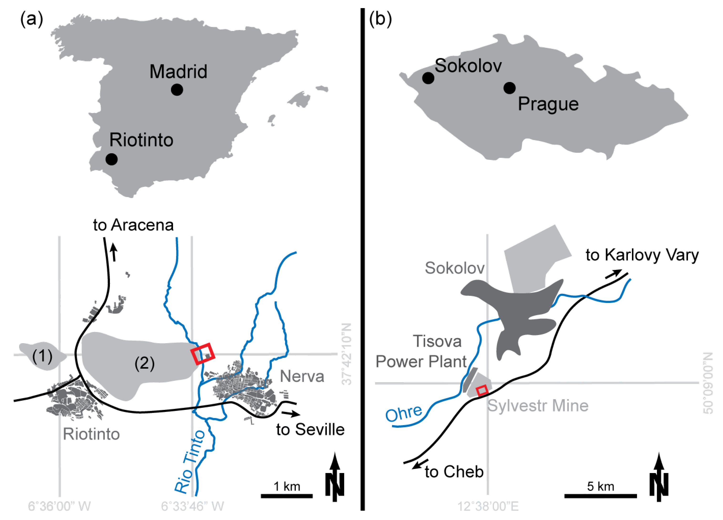
We first present a drone-borne example dataset originating from parts of the mining area of Minas de Riotinto in southern Spain (
Figure 1a). This region hosts one of the giant massive sulphide deposits of the Iberian Pyrite Belt and has been extensively mined for copper and lower amounts of manganese, iron and gold since the Bronze Age. The test site covers one of the gossanous ridges overlying a massive sulphide lens next to Riotinto River. Within the test site, different iron-bearing facies occur, such as the gossan itself, massive sulphide, altered shale and river sediments under the influence of acidic mine drainage (AMD) (Riaza et al. [
25]).
The Iberian pyrite belt is hosted in a north -vergent fold and thrust belt of late Variscan age (Soriano and Casas [
26], Donaire et al. [
27]) extending from east of Setubal/Portugal to north of Seville/Spain. A typical succession starts with a series of phyllites/quartzites, followed by slates, basalt sills, felsic volcanics (rhyolites and dacites) and Culm series (greywackes and slates) (Donaire et al. [
27]). The stratabound, volcanogenic massive sulphide (VMS) lenses are hosted in felsic volcanics of Upper Devonian to Lower Carboniferous ages (Soriano and Casas [
26]). Zones of chloritic and argillitic alteration (Saez and Donaire [
28]) are associated with those lenses. Stockwork zones occur underneath the lenses in the vicinity of faults (Saez and Donaire [
28]). A gossan usually forms in the cap-rock above. The deposit of Riotinto itself is located in a hinge of an E-W trending fold with the fold axis plunging towards E. The studied area of the gossan close to Nerva cemetery expresses the easternmost surface outcrop of the mineralized core zone. There, the highly folded, partly altered lower Culm series rock (slates) is overlain by gossan. Within the Culm, a lens of pyrite-rich massive sulphide with associated argillitic alteration is exposed. Our primary geological target is to differentiate several geological endmembers that cannot be distinguished on an RGB orthophoto and to compare the image spectra to validation spectra measured in situ. We attempt to demonstrate that specific variations in the spectral information acquired by the HSI devices on UAS can be used to distinguish specific mineralogical associations. The proposed test site at Riotinto features a medium relief and was surveyed under nearly ideal illumination conditions.
We provide results from a second test site, the abandoned lignite mine of Sylvestr, which is located in the Eger Graben of the Czech Republic near the city of Sokolov (
Figure 1b). It features a complex and steep relief to test the data processing algorithms under more extreme conditions. The area is surveyed under suboptimal illumination conditions, such as a low Sun-horizon angle. Within the mine, tertiary sediments of the Eger Graben and layers of lignite and petrified wood are exposed. The main lithostratigraphic units occurring in Sylvestr are the Nové Sedlo Formation and the Habartov member of the Sokolov Formation, both characterized by volcanic rocks and lignite-bearing sediments, comprising mainly tuffs, sands and silty clays (Rojik [
29]). Similar to surrounding active and closed mine and dump sites, the study area is largely affected by AMD, indicated by low to intermediate pH values and the presence of pyrite, lignite, jarosite and goethite. This originates mainly in the presence of sulfur within the abundant lignite layers, as well as in hydrothermal deposits along the fault system bordering the basin (Kopackova [
30]). After the stop of the mining activities, the pit was left open, and stream erosion incised deep canyon-like channels into the occurring sediments. This topographic variety combined with a sparse vegetation cover proposed Sylvester mine as the ideal test site for the topographic correction of drone-borne HSl data.
3. Data Acquisition
3.1. Aerial Platforms
The areas were studied by means of HSI techniques and structure-from-motion (SfM) photogrammetry. Each method requires specific preconditions for the aerial platform. While the frame-based HSI requires a stable platform at the time of image acquisition to allow a sufficient integration time, SfM requires a rapid platform in order to acquire numerous RGB pictures having sufficient overlap to compute a digital surface model (DSM).
In general, two types of aerial platforms or UAS are available: (1) fixed-wing systems with the advantage of long flight endurance and fast cruising speeds. So, large areas can be captured within one flight, but their disadvantage is a limited payload capacity. The greater the payload, the bigger is the wingspan. In this context, especially take-off and landing become thrilling with expensive and/or sensitive equipment on-board. Furthermore, a fast shutter speed is needed to get high quality image data. (2) Multi-copters have the disadvantage of limited range and flight time; however, they can carry heavier payloads. Due to their hovering capacities, they are more stable at the point of image acquisition, and also, landing is more controlled (especially important with expensive or sensitive payloads).
Based on the above listed arguments, two different platforms had been applied: (1) a sensefly ebee fixed-wing system with a Canon Powershot S110 RGB camera and maximum flight time of 50 min; (2) an Aibotix Aibot X6v2 hexacopter either equipped with a Rikola Hyperspectral Imager [
6] or a Nikon Coolpix A RGB camera. The Aibot has a maximum flight endurance of 15 min and a maximum payload of 2 kg.
Separate pre-defined flight plans were applied for each UAS to meet the requirements in terms of ground resolution, image acquisition time and image overlap. Both systems store their flight logs internally (flight path and points of image acquisition), so a geo-location of the image data is possible afterwards.
3.2. Sensors
A frame-based hyperspectral camera (Rikola Hyperspectral Imager Rikola Ltd. [
6]) was used for data acquisition. Its low weight of just 720 g makes it perfectly suited for drone-borne surveys. The sensor provides snapshot images covering the VIS-NIR spectral range between 504 and 900 nm. In autonomous mode, up to 50 bands with a spectral resolution of > 10 nm and spectral sampling of 1 nm can be acquired within one flight. The maximum image dimensions account for 1024 × 1011 px. However, the spatial resolution for flight images is 1011 × 648 px to enable the maximum number of spectral bands. The raw data are stored on a Compact Flash (CF)-card in autonomous mode and later converted to radiance using the Rikola Hyperspectral Imager software provided by the manufacturer (Rikola Ltd. [
6]).
SfM photogrammetry was flown with either a Canon Powershot S110 digital camera having a resolution of 12 MP (Spain) or a Nikon Coolpix A with 16-MP resolution (Czech Republic). They provide standard red, green and blue band data that can be complemented by visual real color renderings. A correction for lens distortion was applied within the SfM process.
3.3. Flight-Site Setup
Local setup of the base station and final flight plan is always adjusted on-site due to local and meteorological conditions. Ensuring the maximum safety of the operation and a visual-line-of-sight (VLOS) to the aerial system is the highest premise. The flight parameters of the presented study areas are listed in
Table 1.
A total of six parallel flight lines were planned for photogrammetry in Test Site 1. Line spacing was set to have high overlap of the aerial photographs (85% horizontal and 70% vertical). The hyperspectral survey was performed as a single line profile perpendicular to the gossaneous ridge. Camera positions were set to have about 40% horizontal overlap. In total, 10 hyperspectral scenes were acquired. Three flexible PVC panels colored black, grey and white with known spectra were put down underneath the flight line. These panels are used for calibration purposes in the later processing.
In Test Site 2, the photogrammetric survey was performed in seven parallel flight lines parallel to the direction of the main gully. Line spacing was set to 80% horizontal and 60% vertical overlap at a flight altitude of 60 m. The hyperspectral survey was performed along a single line and follows the channel. The setup of hyperspectral data acquisition is similar to Test Site 1.
4. SfM Photogrammetry
The digital surface model was computed by using a standard structure-from-motion (SfM) algorithm implemented in the available commercial software Agisoft Photoscan. SfM (Turner et al. [
17], Westoby et al. [
20], Eltner et al. [
31]) is a low-cost, user-friendly photogrammetric technique solving the equations for camera parameters and scene geometry using a highly redundant bundle adjustment. The SfM approach was pushed in the 1990s by the upcoming computer vision and the development of automatic feature-extraction and matching algorithms.
A typical SfM workflow towards a final surface model consists of five steps (Westoby et al. [
20], Eltner et al. [
31], Snavely et al. [
32]): (1) detection of characteristic image points (e.g., using SIFT) followed by automatic point matching using a homologous transformation (e.g., using RANSAC); (2) reconstruction of the image acquisition geometry and referencing of the intrinsic coordinate system to available reference points (either GPS or known camera locations) using a iterative bundle adjustment; (3) a dense point matching of the sparse cloud from image network geometry; (4) meshing of the dense point cloud; a digital surface model (DSM) can be obtained from this or the previous step; (5) calculating the textures from the images to compute the rectified orthomosaic.
5. Correction Steps for Drone-Based HSI
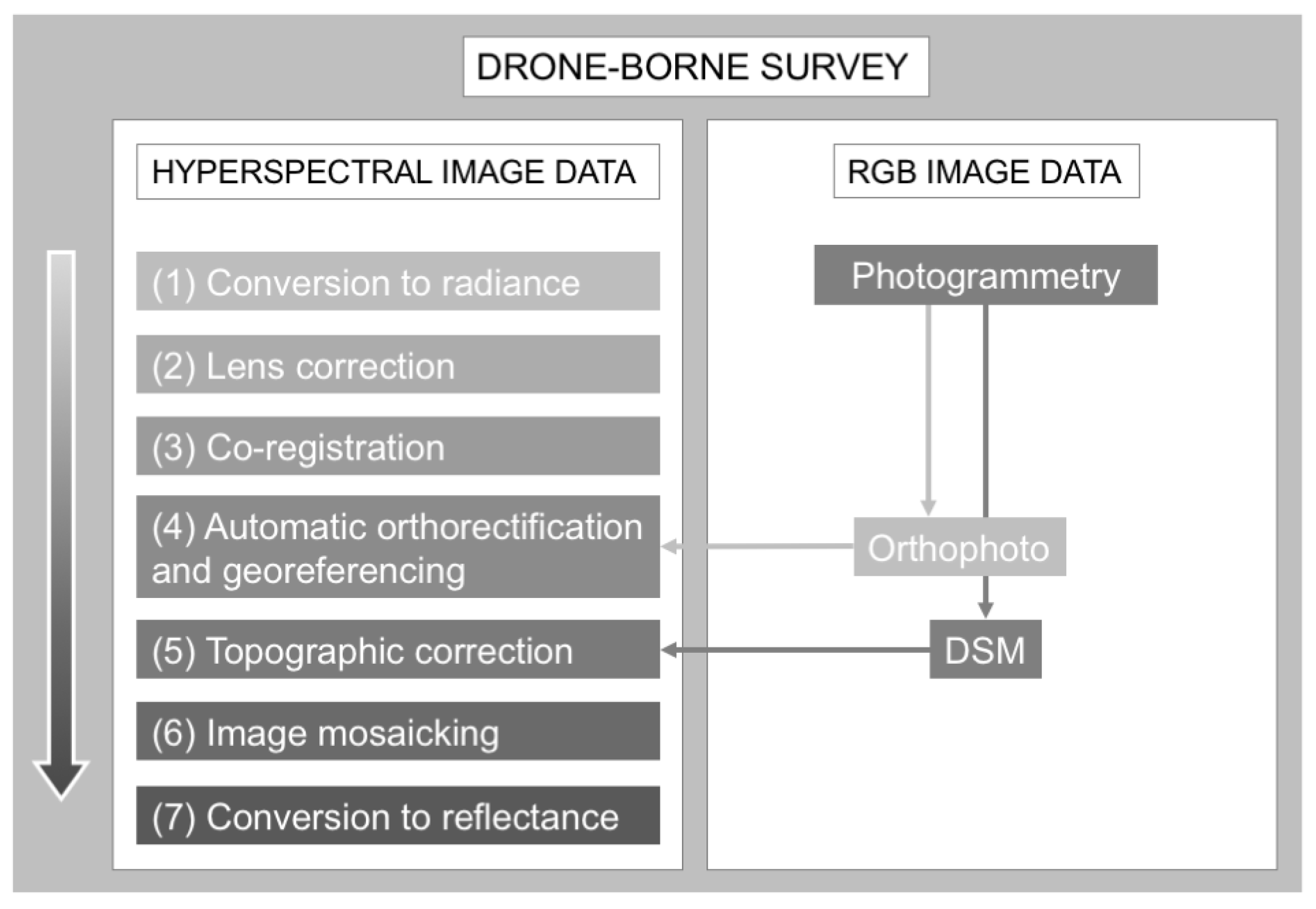
Drone-borne HSI data need a different and more complicated pre-processing chain as air- or space-borne HSI data due to the low acquisition height, difficult calculation and inconstant movement of the platform and, more importantly, the high influence of the micro-relief on illumination and viewing angle. Existing software for processing drone-borne data is often not applicable for hyperspectral images or does not address corrections needed for geological application. Many approaches are related to the use of RGB-images only and are not able to handle the size and especially the data format of hyperspectral imagery. Published approaches for the correction of drone-borne multi- or hyperspectral data are mainly limited to agricultural or environmental applications, assuming a flat topography. However, for geological application, surface geometry is a prominent and crucial factor to consider. Illumination angle changes caused by micro- and macro-relief can distort the spectral appearance of rocks and soils distinctly. This can lead to problematic misinterpretations, as the discrimination of rock or mineral phases is mainly based on subtle changes in the reflectance spectrum. Another important factor concerns the geolocation and orthorectification of the single images. Most available software assumes the use of an IMU, which records the exact position and orientation of the sensor during the acquisition for later correction. Unfortunately, the use of an IMU exceeds the payload of most light-weight UAS and is therefore not feasible. Another possibility is the manual georeferencing using GCPs, which, however, can be very time-consuming for larger UAS surveys. We therefore suggest to automate the geolocation and orthorectification process without the use of an IMU or GCPs. To meet the mentioned challenges, we combined new and known methods in a Python toolbox in a way to process drone-borne HSI data accurately, automatically and as lossless as possible. The processing steps are illustrated in
Figure 2 and are more precisely elaborated afterwards.
5.1. Dark Current Subtraction and Conversion to Radiance
A dark calibration is needed to determine the dark current (DC) of the camera’s sensor. DC equals the noise the camera sensor adds to the signal when translating incoming radiation to digital numbers (DN). If the camera is triggered under completely light-free conditions, this noise becomes visible within the resulting image and can be subtracted from the acquired raw image DN. As the shutter of the camera cannot be closed manually, we use a completely light-blocking plastic foil that is normally used for the transport of OSL (optically-stimulated luminescence) dating samples to prevent incidence light during the DC recording. The image DC subtraction is done with the Hyperspectral Imager software provided by Rikola Ltd. (Rikola Ltd. [
6]). This software is also used to calibrate the image data for vignetting, as well as some camera specific values and to convert the raw DN to radiance.
5.2. Camera Distortion
Distortions caused by internal camera features relate mainly to radial and tangential distortions. Radial distortions are related to the shape of the lens and mostly become visible as a “barrel” or “fish-eye” effect. Tangential distortions can be caused by a non-parallel assembly of the lens in regard to the image plane.
The lens distortion parameters of the Rikola hyperspectral camera were determined using Agisoft Lens, which uses a checkerboard pattern that is projected on a flat screen or printed out. The parameters are listed in
Table 2. At least ten images need to be acquired from different angles and orientations. Using these images, the internal camera parameters, as well as the distortion coefficients can be calculated. The internal parameters can be expressed by the characteristic camera matrix, which includes focal length (fx and fy), skew and center coordinates (cx and cy). The distortion coefficient matrix comprises the radial distortion coefficients k1, k2, k3 and the tangential distortion coefficients p1 and p2. The Rikola Hyperspectral Imager shows a strong radial distortion, but a nearly negligible tangential distortion. The determined parameters are used to correct the lens distortion using the OpenCV undistort function. Hereby, camera matrix and distortion coefficients are used to calculate the relation between the original and distorted camera pixel position. The resulting destination map is used in an inverse mapping algorithm to undistort the raw image (Bradski [
33]).
5.3. Co-Registration
Single spectral bands of one image are acquired with a small temporal difference. Depending on the speed, movement and vibrations of the aerial platform, this results in a spatial shift between the single bands of the HSI data cube. The correction of this mismatch is performed using an image-matching algorithm. We use the SIFT algorithm (Lowe [
34]) for the detection of similar features within the several bands followed by the FLANN algorithm (Fast Library for Approximate Nearest Neighbors, Muja and Lowe [
35]) for matching the detected points. The SIFT algorithm of Lowe [
34] aims to detect local feature vectors within an image, each invariant to image translation, rotation and scaling and partially invariant to affine or 3D projection and illumination changes. The identification is conducted by a staged filtering approach, including extrema detection, keypoint localization, orientation assignment and keypoint descriptor extraction. Due to its robustness to difficult geometric and radiometric conditions, SIFT is a popular tool, e.g., for image registration in photogrammetry, panorama stitching and motion tracking [
34]. The FLANN matching algorithm library was presented by Muja and Lowe [
35]. It contains a range of fast nearest neighbor matching algorithms for high dimensional features and large datasets and provides a routine, which automatically chooses the best method and parameters according to the input dataset.
From the point pairs detected with SIFT and FLANN, an affine transformation matrix, which considers translation, rotation, shift and shear, is calculated and used to correct the mismatch between the single image bands with high precision. Additionally, a subsequent automatic cutting was implemented in order to remove the residual image borders, which originate from the relocation of single bands by the co-registration process.
5.4. Automatic Orthorectification and Georeferencing to the Orthophoto
Similar to the previous step, automatic orthorectification and georeferencing are based on point matching. The SIFT and FLANN algorithms are used to extract matching points between the dataset and a high resolution orthophoto created beforehand using SfM photogrammetry. The quality of the orthophoto regarding spatial resolution and location accuracy is hereby a crucial point to guarantee a successful matching. The matched points are now used to warp and orthorectify the original dataset to the right position. Depending on the level of distortion in the dataset, a polynomial or locally-adaptive transformation can be applied. Hereby, no additional information, such as RPCs (rational polynomial coefficients) or GCPs, is needed.
5.5. Topographic Correction
Topography can have a high influence on the local illumination within an image. The radiance of the same material varies if it is located on a slope oriented towards or away from the sunlight incidence. Thus, it is essential to correct for these effects to retrieve reliable data. We implemented and tested the most common topographic correction methods to aim for an optimal correction result. The methods comprise Lambertian, as well as non-Lambertian methods. For all methods, a digital surface model (DSM) is required, as well as the Sun horizon angle and azimuth present at the acquisition time. These parameters are needed to model the illumination (IL) conditions by:
with incidence angle
i, terrain slope angle
s, solar zenith angle
z, solar azimuth angle
a and terrain aspect angle
o. The calculated illumination (IL) model is the basis for all implemented topographic correction methods.The cosine method is the most common Lambertian approach, which assumes that lower IL is related to higher corrected reflectance and regards the Sun zenith angle. It was introduced by Teillet et al. [
36] and is calculated as:
with
being corrected reflectance and
being original reflectance before topographic correction. As this approach has been seen to over-correct the image in areas with very low IL, Civco [
37] introduced the improved cosine method also considering average IL conditions with:
with
being the mean IL value of the whole study area. Another attempt to reduce the over-correction is the gamma method [
38], which adds parameters for sensor view angle
v on flat and inclined terrain with:
The percent-method is a simple approach for topographic correction proposed in Tizado [
39]. The amount of correction is calculated according to the percent of solar incidence on the Earth’s surface, varying between no correction for direct Sun exhibition to infinite correction for a location in opposition to the solar incidence. Thus, the corrected reflectance is calculated by:
The non-Lambertian Minnaert method is based on Minnaert [
40] and calculated by:
where the Minnaert constant
k is obtained by linear regression of
for each wavelength band. The method was later supplemented for the inclusion of slope by Colby [
41] with:
An empirical-statistical approach named c -factor was published by Teillet et al. [
36]. It is determined by:
where
c is
from the linear regression of
.
5.6. Mosaicking
The georeferenced and topographically-corrected images can now be easily combined into a hyperspectral image mosaic without further transformation. Alternatively, we also provide a tool for the automatic stitching of un-georeferenced images. The overlapping images of a survey are automatically mosaicked without the need of ground control points or any image position information. Again, we use an image matching algorithm based on SIFT and FLANN. This time, a homography transformation matrix is calculated. In addition to the affine parameters, it also considers perspective distortions. Optional illumination correction between the several images can be applied. It uses matching points within the overlap of the images to calculate a regression function, which is afterwards applied to correct brightness differences caused by slightly changing illumination conditions during the acquisition of different images.
5.7. Radiometric Correction
After all geometric and illumination corrections are performed, the hyperspectral radiance image can be converted to reflectance. The influence of the atmosphere is nearly negligible due to the low acquisition altitude. Thus, no common atmospheric correction needs to be applied, as is done for space- or air-borne data. Instead, the empirical line method is recommended. It is a more direct approach using spectrally well-characterized ground reference targets. For that, we use 50 × 50 cm PVC panels in black, grey and white. They feature relatively consistent and flat reflectance spectra in the VNIR spectral range, which were determined using a Spectral Evolution PSR-3500 portable field spectrometer. Other targets, such as characteristic materials within the observed area, can be added by field spectrometer sampling as long as they can be individually resolved in the hyperspectral image. Within the empirical line correction, the reference spectra are compared to extracted image spectra of ground targets to estimate the correction factors for each band. The hyperspectral mosaic is converted to surface reflectance by applying those correction factors. After the conversion to reflectance, an optional spectral smoothing can be applied to remove remaining noise; for this, the Savitzky–Golay filter is recommended (Savitzky and Golay [
42]).
6. Results
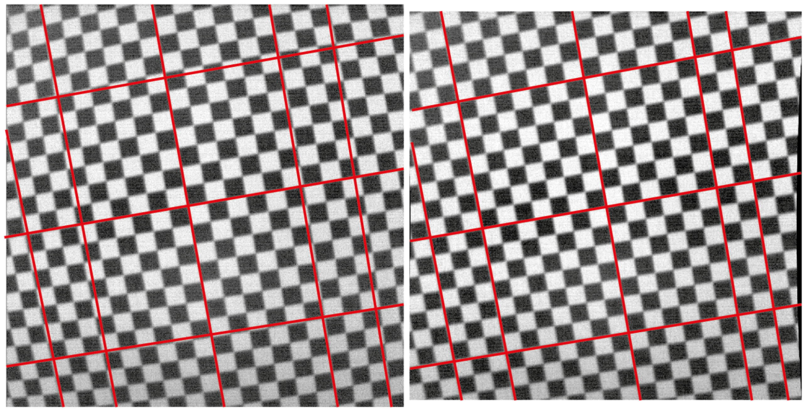
The toolbox presented above is able to perform a fast and reliable correction of the raw data. Every correction step is necessary and improves the dataset towards a useable solution. A reliable hypercube of a single image or a seamless mosaic is the result. Camera distortions were successfully eliminated using a simple lens correction algorithm. The result compared to the distorted image is shown in
Figure 3 with red lines added for better visibility. While a significant barrel distortion is obvious in the uncorrected image, it is completely removed after correction.
The lens corrected image is co-registered to remove the influence of platform shift afterwards. Co-registration is able to correct even high shifts with great accuracy even for bands within different wavelength ranges (
Figure 4a,b). The subsequent residual edge cutting (
Figure 4c) worked well and prepared the single images for subsequent seamless mosaicking.
The preprocessed images were georeferenced and orthorectified before mosaicking. The automatic processing happens with high accuracy despite the differing imaging distances caused by overflying the gossanous ridge. For very low topography, a polynomial transformation is reasonable, for more difficult terrain, a finer adaption to the topography is achieved using a locally-adaptive linear interpolation grid. The automatic georeferencing tool worked well for the orthorectification of single images using polynomial, as well as locally-adaptive transformation. However, the registration of images with the adaptive transformation method shows a distinctly increased fit accuracy compared to the polynomial fitting at the cost of a higher processing time.
Rough terrain surfaces require an appropriate correction for the surface irregular geometry. Thus, all algorithms presented in
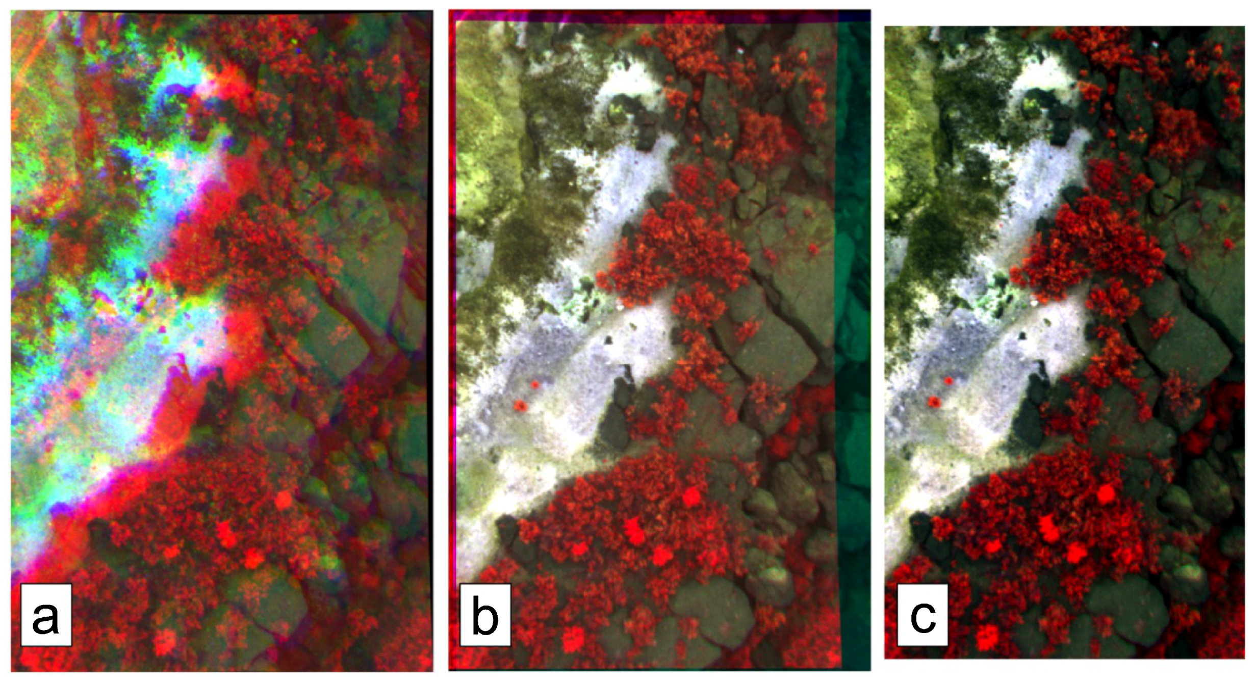
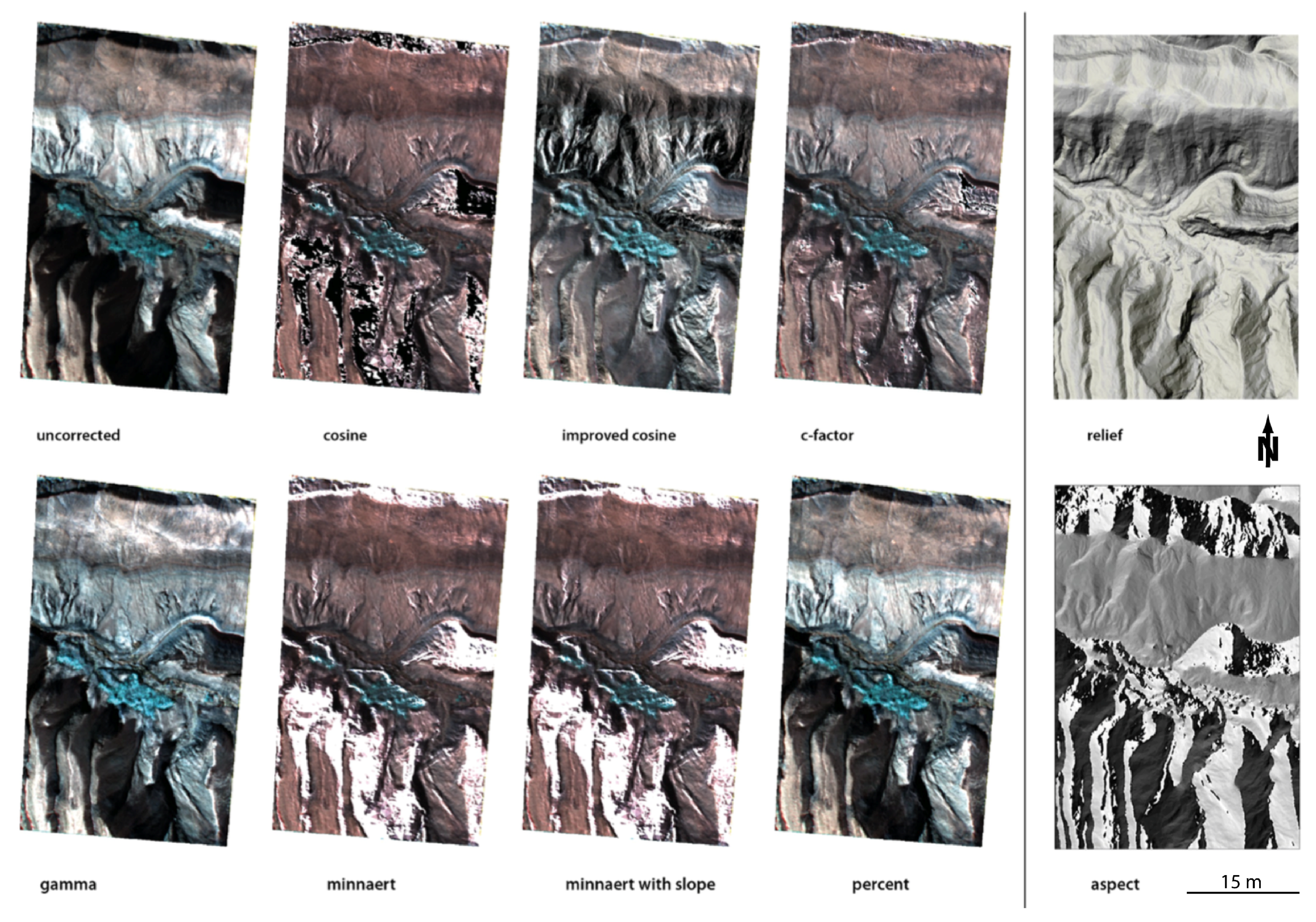
Section 5.5 were tested on the georeferenced images. As the illumination conditions at the Spanish test site were very good with a high Sun angle of 54°, the correction effect is low, and all methods show only slightly different results. Therefore, c-factor, Minnaert and Minnaert with slope are giving the smoothest results, while cosine tends to over-correct values at edges. The improved cosine shows this effect to a much lower extent, while the percent only has a very low to no correction effect at all. To compare the performance of the distinct algorithms under sub-optimal conditions, they were additionally tested on a drone-borne hyperspectral image with extreme illumination differences. In addition to high relief, the images were acquired in the late afternoon, resulting in a Sun horizon angle of 23°. The resulting corrected image for each tested method at Sylvestr mine is displayed in
Figure 5.
The gamma and percent algorithms show only a negligible correction effect. The methods cosine, Minnaert and Minnaert with slope deliver very good results for illuminated parts of the image. However, they fail to correct for the shadowed steep cliffs. Moreover, in the case of the latter two, the algorithms are not able to handle incidence angles over 90 degrees. The improved cosine and c-factor are the only algorithms to correct for the shadowed parts in the image. Nevertheless, improved cosine struggles with immense artifacts especially in the highly illuminated parts, where the incidence angle is around 90 degrees. The only method to correct for both highly illuminated, as well as highly shadowed parts in the image is the c-factor algorithm. Thus, it was therefore used to correct the test site mosaic.
After the successful completion of the previous correction steps, the images can be easily merged to a mosaic. If necessary, a feathering can be applied for a smoother image overlap. The additionally implemented automatic mosaicking algorithm can be used for the stitching of un-georeferenced images without the need for further orientation or geolocation information. It returned precisely-merged mosaics and was able to stitch even images with high topographic influences. Still, the accuracy lies behind the the stitching of already orthorectified images.
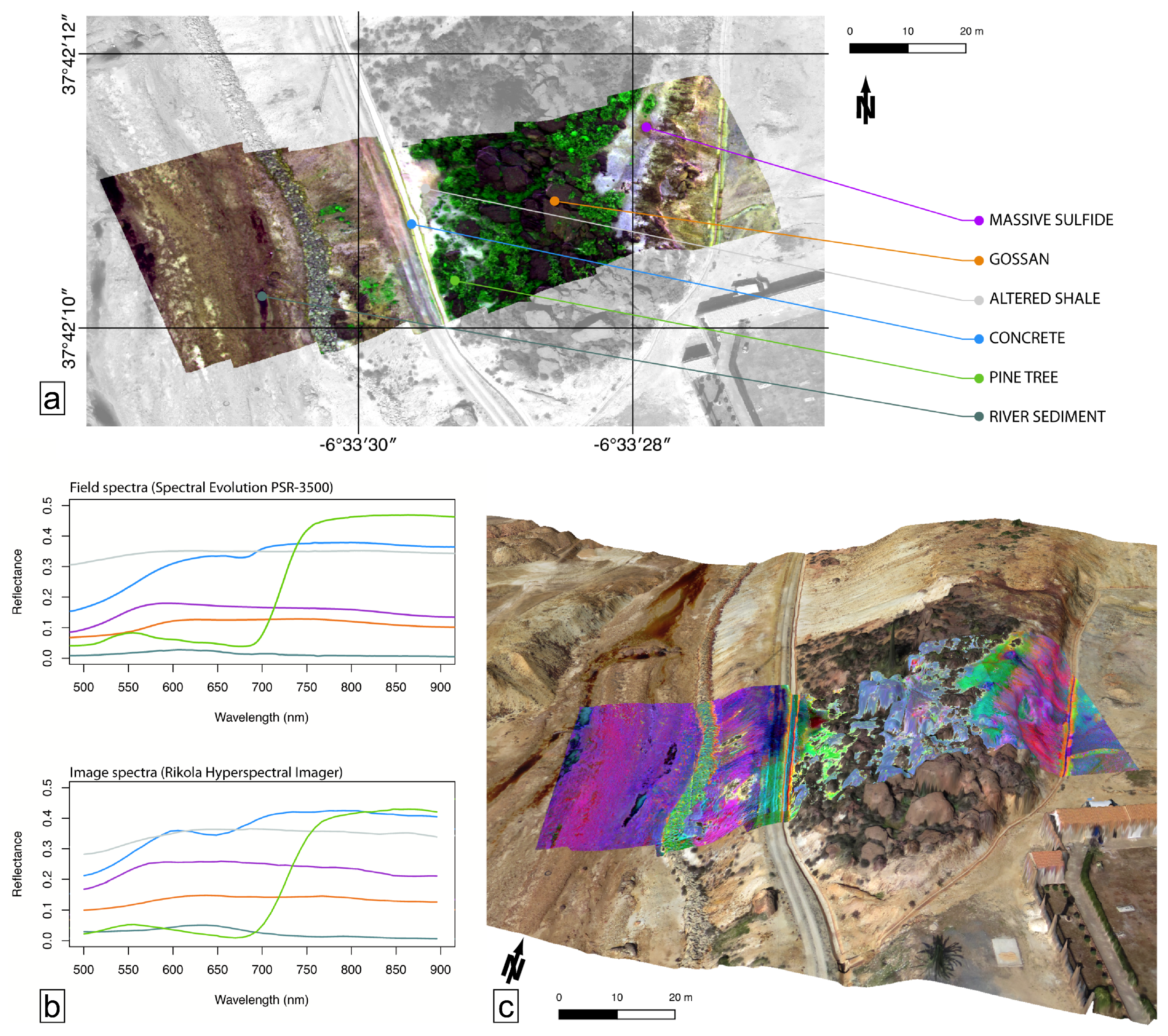
After mosaicking, the image spectra are converted to reflectance. Within most surveys, the white calibration panel was neglected due to over-saturation. However, the empirical line calibration using only the black and the grey calibration panel delivers excellent results, as the image spectra show a very high resemblance to the validation field spectra (see
Figure 6) regarding both shape and intensity. For a subsequent spectral smoothing, we applied a Savitzky–Golay filter with a window size of five and a polynomial degree of two.
Vegetation can be easily distinguished in the spectral data by the so-called red edge around 700 nm. Therefore, it can be easily masked out using the Normalized Differentiated Vegetation Index (NDVI). In contrast, the main lithological components of the test site show only very low differences and nearly no highly distinctive absorption features in the VNIR spectral range. This accounts both for the field validation spectra, as well as the image spectra. Nevertheless, small differences in intensity, convexity and slope of the spectral curve are present. They can be used to distinguish several lithological endmembers. Therefore, gossan, nearby occurring massive sulfide and altered shale, as well as artificial concrete structures and river sediments can be clearly distinguished from each other (see
Figure 6) using the principal components of the hyperspectral image. This differentiation is impossible from the RGB orthophoto.
7. Discussion
The presented processing chain for drone-borne HSI data works robustly and is able to correct raw data to reflectance with the least loss of spectral information. Lens correction, band registration and residual edge cutting are eligible to remove distortions caused by both the camera system and movement of the aerial platform.
Automatic georeferencing, orthorectification and mosaicking are time saving compared to the manual approach or using GCPs. The implemented algorithms work reliable even for complex geometries and with high accuracy. Slightly distorted data, such as images over a low-relief landscape, can be treated quickly using homographic or polynomial transformations. Even data with high local distortions caused by the underlying topography, typical for drone-borne geological imagery, can be processed. A subsequent topographic correction is highly recommended for sites with high relief or sub-optimal illumination conditions during data acquisition. The best results were derived from c-factor, Minnaert and Minnaert with slope. However, only c-factor can be applied to images with highly shadowed parts and is therefore recommended for the topographic correction of drone-borne HSI data.
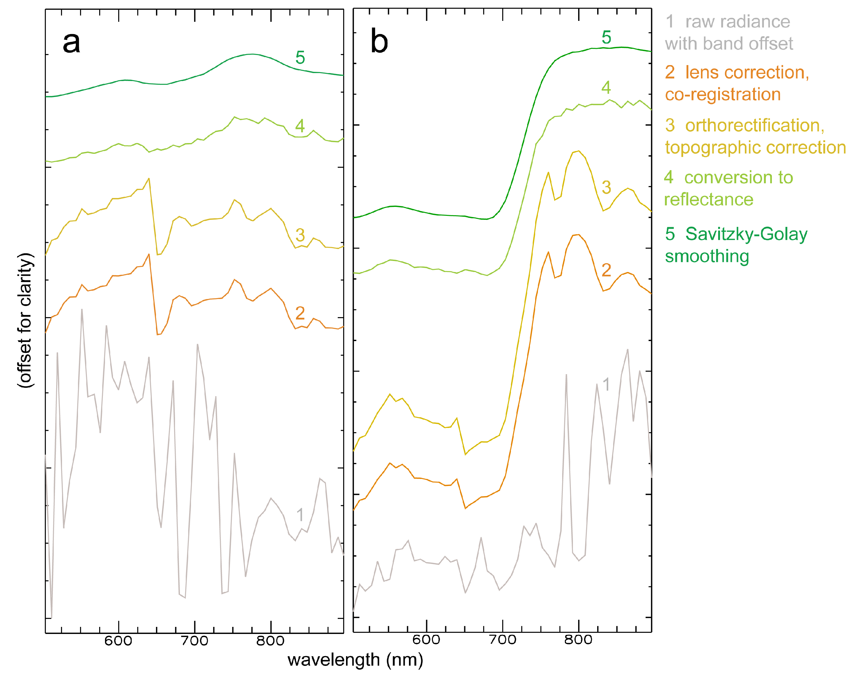
Figure 7 shows the progress of data pre-processing at two exemplary pixel spectra. The correction of the lens parameters and the band registration achieve a distinct improvement of the spectral shape, which is mainly explainable by the now aligned corresponding pixel values along the spectral dimension axis. Orthorectification and topographic correction do not influence the shape of the spectral curve. While orthorectification only influences the spatial pixel positioning, topographic correction corrects for the relative spectral intensity between pixels without changing the spectral shape itself. The conversion to reflectance finally achieves a reliable and completely corrected spectrum. An optional spectral smoothing reduces remaining noise. After correction, the absorption features of ferrous and ferric iron (around 650 and 900 nm) within the spectrum of the iron-rich gossanous sample become clearly visible, as well as the characteristic vegetation spectrum with the red edge around 700 nm for the pine tree sample pixel. The comparison of the different correction steps distinctly reveals the importance of all correction steps. Further, it highly recommends their use to achieve reliable and highly accurate image spectra, which are crucial for the discrimination of geological targets.
The calculation of reflectance by empirical line conversion yields smooth spectra with a high resemblance to measured validation spectra (see
Figure 6). Interestingly, the white calibration panel turned out to be unsuitable for the conversion to reflectance due to over-saturation in most of the surveys. This originates from the integration time used during the image acquisition. Integration time is always adjusted for an optimal exposure of the complete survey area having a much lower reflectance than the white panel. Adding additional panels in different shades of grey would be a possible straight-forward solution. Resulting reflectance spectra of the corrected image data feature low noise and show a high resemblance to the validation field spectra.
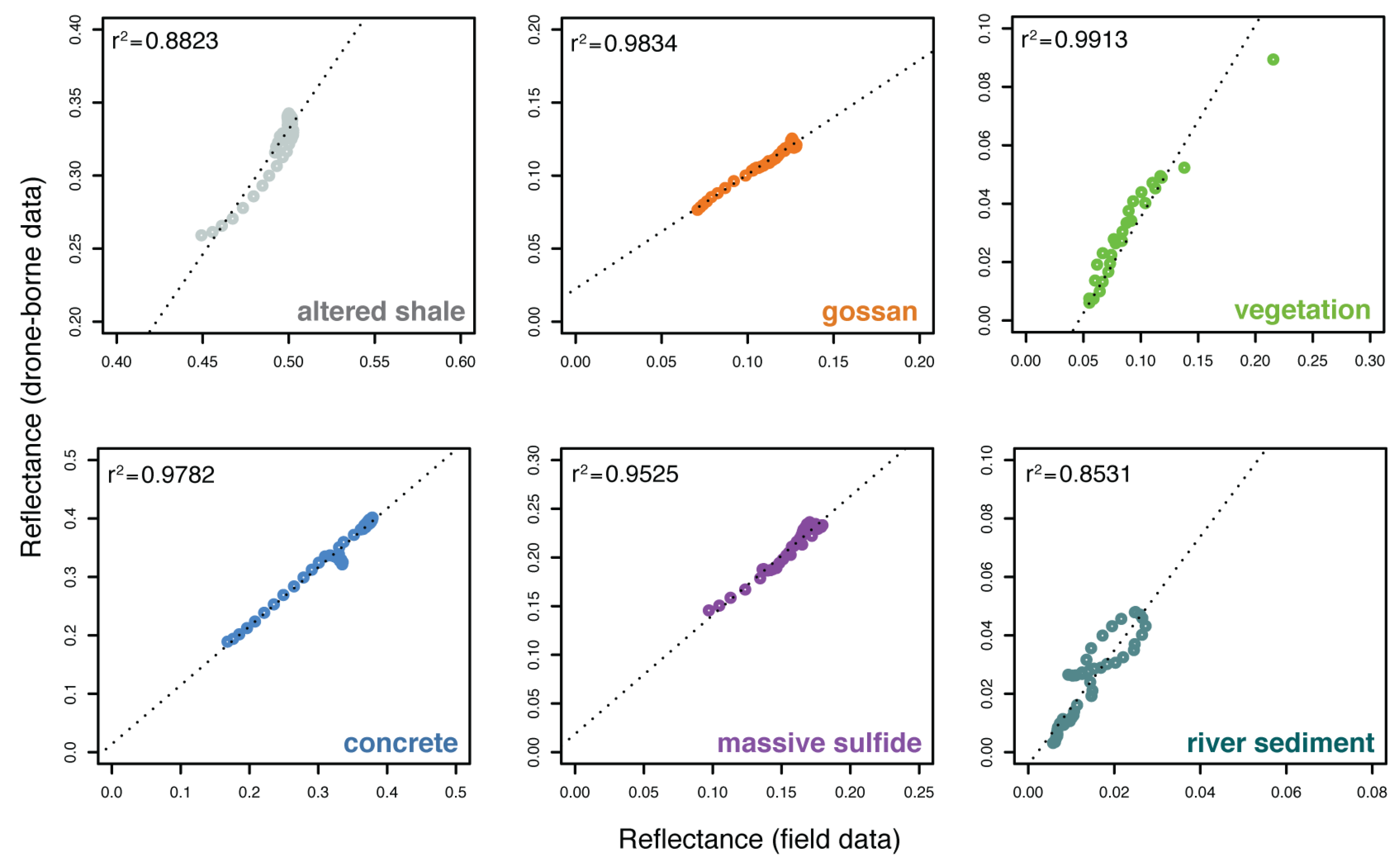
Figure 8 shows a comparison of the spectral reflectance of field and drone-borne spectra for six sample materials. Results stress a linear correlation between both sensors. The spectral responses are similar for most of the targets. However, differences in overall reflectance intensity occur due to non-identical measurement conditions and the spatial coverages of the sensors. Another issue to be considered is that, although the position error of the measurement spots seems negligible, it can highly affect the spectral response in heterogeneous materials.
The detected VNIR range of the spectrum features only a low amount of characteristic mineral-related absorption features, such as for iron oxides. However, different iron-bearing facies occurring at the test site could be distinguished. Therefore, massive sulphides and gossan show a slight absorption feature around 650 nm (
Figure 6), which is not abundant in the spectrum of sediment from Riotinto River. This feature is characteristic for the charge transfer of Fe
3+ and Fe
2+ and can be related to Fe
3+-bearing minerals, such as goethite [
43]. In addition, most materials in the scene feature a Fe
2+ absorption indicated by a broad and shallow absorption around 900 nm. Depending on the actual mineralogical composition, the position of the absorption can be shifted or show differing intensities. This can be used to differentiate between the different lithologies. These small spectral differences enable one to distinguish even between spectrally quite similar iron-bearing materials.
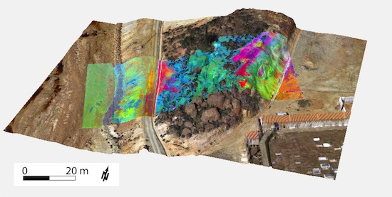
The results stress the use of drone-borne HSI data as valuable support for mapping alteration and enrichment zones. It further indicates the abilities to map different iron minerals, e.g., for acid mine drainage. The automated workflow enables an easy processing of large flight surveys and a much faster provision of hyperspectral imagery compared to a manual approach. Due to the precise orthorectification and georeferencing, as well as the high spatial resolution of HSI data, orthophoto and DSM, hyperspectral 3D models can be created to visualize the mapping results. Hereby, the HSI results can be set into spatial relation with topographical and structural features.
The presented toolbox is not especially designed for Rikola hyperspectral data, but can be easily adapted for any frame-based hyper- or multi-spectral sensor on the market. Additionally, the application of the corrected drone-borne hyperspectral mosaics is not limited to lithological or mineral mapping.
8. Conclusions
For the first time, we proved that drone-borne HSI data can be used in geological studies. We further presented a toolbox including all crucial steps for the pre-processing of drone-borne HSI data for geological applications. Results have the advantage of both high spectral similarity to validation field spectrometer measurements and high spatial resolution. The presented workflow ensures a proper and careful pre-processing, which is important to obtain reliable hyperspectral reflectance data. It shows excellent performance for frame-based hyperspectral images and was tested on data acquired with a common Rikola hyperspectral drone-borne sensor. In addition to sensor- and platform-specific geometric distortion corrections, a topographic correction step is implemented for rough terrain surfaces. We recommend the use of the c-factor-algorithm here. Further, panels in different shades of grey should be preferred over using a white panel to convert radiance to reflectance due to the generally low reflectance of geologic materials.
Despite the low number of mineralogy-related characteristic absorption features in the VNIR spectral range, a differentiation of lithological endmembers is possible due to small differences in the slope, convexity and intensity of reflectance. We proved, e.g., that the corrected HSI data are sensitive enough to distinguish different iron-bearing facies. Thus, we highly recommend the use of the presented correction steps for drone-borne HSI data to ensure an image result highly accurate in geometry, location and spectral information.
Additionally, we highly endorse the increased use of drone-borne HSI data for geological aims, as they show a high potential for fast and accurate mapping of small-scale alteration and enrichment zones. However, their applicability is not limited to mineral exploration, but can comprise and support any other geological and environmental studies.


