Estimation of Wheat LAI at Middle to High Levels Using Unmanned Aerial Vehicle Narrowband Multispectral Imagery

Abstract

Leaf area index (LAI) is a significant biophysical variable in the models of hydrology, climatology and crop growth. Rapid monitoring of LAI is critical in modern precision agriculture. Remote sensing (RS) on satellite, aerial and unmanned aerial vehicles (UAVs) has become a popular technique in monitoring crop LAI. Among them, UAVs are highly attractive to researchers and agriculturists. However, some of the UAVs vegetation index (VI)—derived LAI models have relatively low accuracy because of the limited number of multispectral bands, especially as they tend to saturate at the middle to high LAI levels, which are the LAI levels of high-yielding wheat crops in China. This study aims to effectively estimate wheat LAI with UAVs narrowband multispectral image (400–800 nm spectral regions, 10 cm resolution) under varying growth conditions during five critical growth stages, and to provide the potential technical support for optimizing the nitrogen fertilization. Results demonstrated that the newly developed LAI model with modified triangular vegetation index (MTVI₂) has better accuracy with higher coefficient of determination (R_c² = 0.79, R_v² = 0.80) and lower relative root mean squared error (RRMSE = 24%), and higher sensitivity under various LAI values (from 2 to 7), which will broaden the applied range of the new LAI model. Furthermore, this LAI model displayed stable performance under different sub-categories of growth stages, varieties, and eco-sites. In conclusion, this study could provide effective technical support to precisely monitor the crop growth with UAVs in various crop yield levels, which should prove helpful in family farm for the modern agriculture.

1. Introduction

Leaf area index (LAI) is a key parameter that determines the photosynthesis, respiration, and transpiration of vegetation [1,2]. Real-time monitoring of the LAI for crops can not only help to obtain the status of health and nutrients, but also provide effective technical support in fertilizer application and water management [3].

Remote sensing (RS) techniques are widely used in agriculture and agronomy [4]. The common method of monitoring crops LAI is to use some data (vegetation index, degree of coverage, and so on) acquired by remote sensing sensors on ground-based [5], satellite or airborne [6,7] platforms. However, the ground platform is used at individual locations and thus has low efficiency for wall-to-wall mapping; satellite data are often difficult in meeting the requirements of spatial and temporal resolutions [8,9]; manned airborne campaigns can acquire high spatial resolution data over relatively large areas, but they are costly. Unmanned aviation vehicles (UAV_S) have emerged in the last decades to overcome the deficiencies of the above platforms, especially for precision agriculture, because UAV can acquire data with high temporal frequency and spatial resolutions at a low cost [8,9,10]. A recent study [11] compared three types of data from the ground-based ASD Field Spec Pro spectrometer (Analytical Spectral Devices, Boulder, CO, USA), UAVs mounted ADC-Lite multi-spectral sensor, and GaoFen-1 in retrieving soybean LAI. It found that UAVs mostly has the same high accuracy with the ASD hyperspectral spectroradiometer.

Due to the above advantages, UAVs has been used in an increasing number of studies to estimate LAI for vegetation, mainly through the vegetation indices (VIs) derived from the reflectance of RGB digital cameras attached to the UAVs [11,12]. For example, Chianucci [12] calculated the VI_S at the red, green and blue bands from the UAV true color digital image to estimate the beech forest LAI. Despite those efforts, the accuracy of predicting LAI was not high [11,12]. This could be attributed to the consumer-grade digital cameras used in these studies. These cameras normally capture true-color imagery with three bands (blue, green, and red) in the visible spectrum range. However, considerable research has shown that the vegetation reflectance in the NIR region is more strongly influenced by LAI than that in the visible region [13]. Therefore, a few studies have attempted to develop sensors that substitute one of the blue, green, or red bands with a NIR band. For example, Hunt et al. [14] acquired NIR-green-blue digital photographs from unmanned aircraft, and then proposed the GNDVI (Green Normalized Difference Vegetation Index) on the green and NIR channels for monitoring crop LAI. However, their sensor had just three bands.

Some studies attempted to increase the number of bands by integrating several cameras in one platform, which, however, can pose challenges in image preprocessing. For example, Lelong et al. [15] adapted filters on commercially-available digital cameras (Canon EOS 350D and Sony DSC-F828) to design a new four-spectral-bands sensor (blue, green, red, and NIR), and they acquired the better prediction with RMSE = 0.57 and R² = 0.82. However, they reported that the data pre-processing was quite complex, and the data quality needs to be improved.

These studies mostly examined only the NIR band at the high reflectance “plateau” (around 720–850 nm) and developed corresponding VIs for estimating LAI. However, other NIR bands, especially the red-edge bands, could also be highly useful for predicting LAI [13]. An urgent need exists to test the ability of the UAVs with sensors of more bands, especially with red edge and NIR bands, to estimate LAI. Only a few studies have used UAV multispectral imagery that include red edge and NIR bands for applications such as the seed management [9], olive disease monitoring [10], pasture variations identification [16], and conifer forest carotenoid content estimation [17]. Furthermore, UAVs is a promising remote sensing platform that gained more and more attention for crops. For example, Jin et al. [18] estimate wheat plant density from UAV RGB images. Zhou et al. [19] predicting grain yield in rice using multi-temporal vegetation indices from UAV-based multispectral and digital imagery.

The LAI of crops at the mature stage can reach as high as 7, and the LAI level near which optical remote sensing imagery usually have the saturation problem [19]. Another research gap is that some previous studies in UAV-based estimation of crop LAI often focused on a few growth stages. For example, Hunt et al. [14] only acquired the image of winter wheat on 4th May at the flowering stage. To the best of our knowledge, except Lelong [15] and Potgieter [20], no studies have used UAVs to estimate crops LAI across the whole critical growth period, which can span a large LAI range. In addition, most of the researchers often estimate wheat LAI using normalized differential vegetation index (NDVI). It is well-known that NDVI is one of the most extensively applied VIs for estimating LAI, but merely effective at relatively low LAI values [21]. Later, many studies proposed some effective VI_S to estimate LAI, e.g., the enhanced vegetation index (EVI) [22], the modified triangular vegetation index (MTVI₂) [23], the (optimized) soil adjusted vegetation index (SAVI and OSAVI) [24,25], but these VIs were mostly developed using satellite or airborne sensors. In addition, it is very essential when aiming to use an empirically-optimized VIs model to estimate growth parameters such as LAI using UAV images. There is an urgent need to assess the performance of commonly used VIs from UAV narrow multispectral sensor for estimating crop LAI across all different growth stages.

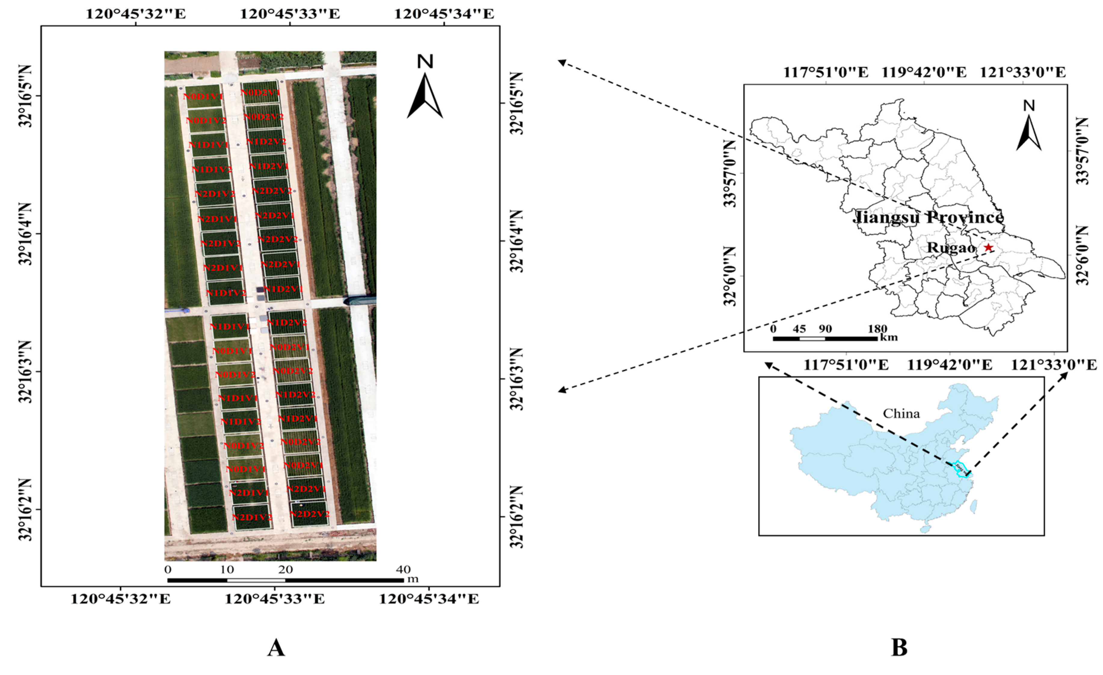
Wheat is the main cereal crop in the world. The number of large wheat family farms is rapidly increasing in China, which need the accuracy and frequent monitoring of growth status to guide the management of fertilizer and water [26]. UAV, due to its low cost, high efficiency, flexible altitude and on-demand adjustment of the testing time, has certainly evolved as the appropriate tool in modern family farms [27].

Our study has the following objectives: (1) to quantify the relationship between wheat LAI and various VIs from the narrowband multispectral imagery; (2) to infer the most powerful VIs over the wide range of growth conditions; (3) to examine the sensitivity of the VIs to LAI at the middle to high levels; (4) to evaluate the generality of VIs for LAI estimation when using independent test dataset with different cultivars, densities, and nitrogen rates during the critical growth period, which would provide the potential technical support for effectively monitoring crop growth in the management and tactics of decision-Nitrogen on the farm scale.

2. Materials and Methods

2.1. Experimental Design

Two field experiments were conducted involving different N application rates, planting densities and winter wheat cultivars (Triticum aestivum L.) in two growing seasons in the town of Baipu town, Rugao city, Jiangsu province, China (120°45′E, 32°16′N) (Figure 1). The detailed experimental design is described below:

Experiment 1 was conducted in a single season from 2013 to 2014 with the sowing date of 28 October 2013. Two winter wheat cultivars, ‘Shengxuan 6’ and ‘Yangmai 18’, were selected to represent different canopy structure (planophile and erectophile types), respectively. Three N application rates (0, 150 and 300 kg/ha as urea) and two planting densities (3.0 × 10⁶ plants ha⁻¹, and 1.5 × 10⁶ plants ha⁻¹) were applied. A split design was used with three replications for all 36 plots with every plot size of 35 m². Other agronomic management was conducted according to the local wheat production practices. Soil organic matter was 24.60 g/kg, available N was 150.41 mg/kg, total nitrogen was 1.87 g/kg, available phosphorus was 57.84 mg/kg and available potassium was 96.32 mg/kg. The basal fertilizer was applied on 26 October 2013, including 120 kg/ha P₂O₅, 120 kg/ha K₂O and three N application rates (0, 75 and 150 kg/ha as urea). Compound fertilizer was applied on 8 March 2014, including three N application rates.

Experiment 2 was conducted with the sowing date of 31 October 2014, and it was a duplicate of Experiment 1 in the 2014–2015 seasons. The soil type is loam soil, and we measured the soil conditions before sowing. soil organic matter was 18.90 g/kg, available N was 100.41 mg/kg, total nitrogen was 2.07 g/kg, available phosphorus was 34.00 mg/kg and available potassium was 90.00 mg/kg. The basal fertilizer was applied on 30 October 2014, including 120 kg/ha P₂O₅, 120 kg/ha K₂O and three N application rates (0, 75 and 150 kg/ha as urea). Compound fertilizer was applied on 5 March 2015, including three N application rates.

In this study area, the average annual temperature was 16.59 °C with the highest and lowest annual temperature as 38.10 °C and −5.57 °C, respectively. The average annual rainfall was 927.53 mm, and we did not consider the effect of water, because rainfall could meet the needs of wheat growth.

2.2. Data

2.2.1. The UAV System

The UAV system (UAV) used in this study includes the ARF-MikroKopter UAV with eight rotors, an MC-32 remote controller, a Thinkpad laptop, and a six-channel narrowband multispectral camera (MiniMCA-6, Tetracam, Inc., Chatsworth, CA, USA), as shown in Figure 2. The specific parameters of the UAV and the sensor are shown in

Table 1. The parameters for the UAV of ARF-MikroKopter.

Parameter	Value
Weight	2050 g
Size	73 × 73 × 36 (W × L × H) cm
Battery 4s/5000	520 g
Maximum payload	2500 g
Flight period	8~41 min
Temperature range	−5 °C~35 °C

and

Table 2. The parameters for the sensor of Tetracam Mini-MCA6.

Channel	Wavelength (nm)	Band Width (nm)	Exposure Proportion (%)
Master (0)	550	10	70
Slave 1	ILS		130
Slave 2	490	10	120
Slave 3	671	10	100
Slave 4	700	10	100
Slave 5	800	10	80

.

2.2.2. Data Acquisition and Processing

Imagery from UAV: the ARF-Mikro Kopter UAV flighted with the Mini-MCA6 multispectral sensor was performed to take images with spatial resolution of 8.125 cm at 150 m altitude. We took the image of the wheat at the five critical stages including the jointing (15 March 2014 and 13 March 2015), booting (9 April 2014 and 9 April 2015), heading (15 April 2014 and 17 April 2015), anthesis (23 April 2014 and 24 April 2015) and grain filling (6 May 2014 and 9 May 2015) stages.

LAI from LI-3000: To be synchronous with the imagery, we took 30 wheat stems from each plot as one sample, separated the green leaves, used a LI-3000 leaf area meter to scan the green leaf area. We total have 36 plots, which the length and width are 7 m and 5 m. The number of stems in one meter length in each plot was counted manually. Based on the Formula (1), the LAI of population was calculated.

LAI = 1/D × B × A/C × 10⁻⁴

(1)

D was the distance between two rows of wheat; B was the number of stems in one meter; A was the leaf area of sample; C was the number of stems of sample.

Pre-processing of the image: We pre-processed the imagery by conducting: (1) noise elimination [28], (2) vignette reduction [28], (3) lens distortion correction [29,30,31], (4) band registration [32], (5) radiometric calibration [33], and (6) background removal [34]. We set 30 ground control points in the experimental area, and used X900 GNSS to determine the geographic coordinates. The horizontal direction of the error can be controlled within 1 cm, the vertical error can be controlled within 2 cm.

Calculation of VIs: We randomly combined every two of the 5 wavebands (490 nm, 550 nm, 671 nm, 700 nm, and 800 nm) to construct VIs, and the bands were selected based on the relationship between the vegetation index and the LAI with higher coefficient of determination, the selected vegetation indices were shown in

Table 3. Algorithms and references of all the possible VI_S.

VIS	Algorithm	Ref.
RVI	R800/R700	[35]
NDVI	(R800 − R700)/(R800 + R700)	[36]
MTVI2	1.5 × (1.2 × (R800 − R550) − 2.5 × (R700 − R550))/(2 × (R800 + 1)2 − (6 × R800 − 5 × R700)0.5 − 0.5)0.5	[23]
SAVI	1.5(R800 − R700)/(R800 + R700 + 0.5)	[24]
GBNDVI	R800 − (R550 + R490)R800 + (R550 + R490)	[37]
RDVI	(R800 − R700)(R800 + R700)0.5	[38]
GNDVI	(R800 − R550)/(R800 + R550)	[39]
MSR	(R800/R700 − 1)/(R800/R700 + 1)0.5	[40]
EVI	2.5 × (R800 − R700)/(1 + R800 + 6 × R700 − 7.5 × R490)	[22]
DVI	R800 − R700	[41]

.

2.3. Data Analysis and Application

The quantitative relationship between the VIs and the LAI was analyzed, and the optimal LAI model was selected based on the regression of the linear, power or exponent functions on the coefficient of determination (Rc²), and the new developed model was calibrated with the data from Experiment 2. The constructed LAI model was validated with the data from Experiment 1. The relative root mean square error (RRMSE) (Equation (2)) and coefficient of determination in the validation (Rv²) were calculated to assess the accuracy of the VI-derived model. The sensitivity of all combinations of VI_S versus LAI was evaluated by the index of noise equivalent (NEΔLAI) [42] (Equation (3)). A higher NEΔLAI value indicates the lower sensitivity with LAI, while a lower NEΔLAI value indicates the higher sensitivity.

$$\mathrm{RRMSE}=\sqrt{\frac{1}{\mathrm{n}}\times {\displaystyle {\sum }_{\mathrm{i}=1}^{\mathrm{n}}{{\displaystyle (\mathrm{Pi}-\mathrm{Qi})}}^2}}\times \frac{1}{\mathrm{Qi}}$$

(2)

$$\mathrm{NE}\Delta \mathrm{E}\Delta \mathrm{L}=\frac{\mathrm{RMSE}\left\{\mathrm{VIvs}.\mathrm{LAI}\right\}}{\mathrm{d}(\mathrm{VI})/\mathrm{d}(\mathrm{LAI})}$$

(3)

$$\mathrm{bias}=\frac{{\displaystyle {\sum }_{\mathrm{i}=1}^{\mathrm{n}}(\mathrm{Qi}-\mathrm{Pi})}}{\mathrm{n}}$$

(4)

where n is the number of LAI samples, P_i is the estimated LAI value, Q_i is the observed LAI value, and VIs is all the possible represented vegetation indices, RMSE {VI vs. LAI} is the root mean square error of the second-order polynomials function and the actual LAI value, and d(VI)/d(LAI) is the first derivative of this function.

3. Results

3.1. Changes of Canopy Reflectance and LAI at Different Growth Stages under Varied Nitrogen Rates

The data from Experiment 2 were taken as an example to demonstrate the variation of the canopy spectral reflectance (Figure 3) and the LAI (

Table 4. The variation of LAI at different growth stages under varied nitrogen rates.

Growth Stage	LAI at N0			LAI at N1			LAI at N2
	Min.	Max.	Ave.	Min.	Max.	Ave.	Min.	Max.	Ave.
Jointing	0.80	1.63	1.15	1.44	2.76	2.14	1.56	3.25	2.63
Booting	1.17	3.26	2.16	3.88	7.04	5.25	5.51	7.99	6.71
Heading	1.07	2.75	1.74	3.82	6.73	5.10	5.28	7.98	6.81
Anthesis	0.98	2.55	1.69	3.78	6.65	5.00	5.09	7.64	6.29
Grain filling	0.84	2.25	1.38	2.63	4.80	3.82	3.24	7.35	4.93

Note: Min. stands for minimum value; Max. stands for maximum value; Ave. stands for average value. N0, N1 and N2 represent three N application rates, 0, 150 and 300 kg/ha as urea, respectively.

) with the five critical growth stages of wheat.

The results showed that the canopy reflectance varies with the five critical growth stages for all the 5 wavelengths. The NIR waveband of 800 nm, the maximum value of reflectance, was with the greatest variation among the 5 narrow bands. Furthermore, the wavelength at 800 nm demonstrated the trend of initial increase and later decrease with the highest reflectance at the booting stage. The other 4 bands (490 nm, 550 nm, 671 nm, and 700 nm) had small variation from the jointing to grain filling stage with the reflectance values low less than 0.12.

Table 4 showed that the LAI tended to first increase and then decrease along the growth stage, reaching the maximum at booting stage. And the similar trend displayed in varied nitrogen rates of N0, N1, and N2. LAI increased in the increasing nitrogen rate with N2 as the maximum, which is consistent in two varieties.

3.2. Quantitative Relationships between LAI and VI_S in Wheat

Based on the data of Experiment 2, 10 commonly used VIs for LAI estimation were selected to calculate the quantitative relationship, then the most powerful VIs with higher coefficient of determination (Rc²) were selected in

Table 5. Quantitative relationship between LAI and VIs from UAVs image.

Number of Bands	VIs	Equation	Rc2	Rv2	RRMSE
Two bands	RDVI (800, 700)	y = 16.79x − 4.44	0.79	0.78	26
	DVI (800, 700)	y = 18.32x − 2.25	0.79	0.65	32
	NDVI (800,700)	y = 0.08e4.97x	0.79	0.68	31
	GNDVI (800, 550)	y = 0.03e6.30x	0.78	0.53	40
	RVI (800, 700)	y = 0.61x − 0.94	0.78	0.66	34
	SAVI (800, 700)	y = 17.01x − 6.54	0.78	0.78	59
	MSR (800, 700)	y = 2.65x − 2.04	0.75	0.67	33
Three bands	MTVI2 (550, 700, 800)	y = 12.10x − 1.93	0.79	0.80	24
	EVI (490, 700, 800)	y = 13.15x − 2.86	0.78	0.82	25
	GBNDVI (490, 550, 800)	y = 0.10e4.75x	0.77	0.42	47

Note: Rc² and Rv² indicate the coefficient of determination in calibration and validation, respectively. RRMSE stands for relative root mean square error.

. Finally, the LAI model was validated and tested by the data of Experiment 1. The calibration indicated that the optimal two-band VIs of 800 nm and 700 nm have better performance with Rc² of 0.79, while the optimal three-band MTVI₂ was superior to others with Rc² as 0.79. Further, the validated results showed that two bands-RDVI and three bands-MTVI₂ have better performance in monitoring of LAI on the UAV_S, with MTVI₂ as the best.

3.3. Evaluation of the Constructed LAI Model in Wheat

3.3.1. Comparison with the Ground Hyperspectral LAI Model

Furthermore, we compared the UVAs derived model with that from the ground based Field Spec 4 ASD spectrometer (

Table 6. Quantitative relationship between LAI and VIs from Field Spec 4 ASD.

Number of Bands	VIs	Equation	Rc2	Rv2	RRMSE
Two bands	RDVI (800, 700)	y = 14.37x − 3.03	0.79	0.83	22
	DVI (800, 700)	y = 16.15x − 1.46	0.82	0.88	19
	NDVI (800,700)	y = 0.16e4.29x	0.81	0.75	27
	GNDVI (800, 550)	y = 0.06e5.44x	0.80	0.71	35
	RVI (800, 700)	y= 0.68x − 0.83	0.81	0.77	26
	SAVI (800, 700)	y = 13.68x − 4.09	0.77	0.83	49
	MSR (800, 700)	y = 2.69x − 1.56	0.78	0.75	26
Three bands	MTVI2 (550, 700, 800)	y = 12.10x − 1.93	0.79	0.83	22
	EVI (490, 700, 800)	y = 11.62x − 2.08	0.81	0.85	22
	GBNDVI (490, 550, 800)	y = 0.24e4.05x	0.81	0.71	42

Note: Rc² and Rv² indicate the coefficient of determination in calibration and validation, respectively. RRMSE stands for relative root mean square error.

). The result indicated that the difference of accuracy for the model was not substantial in the coefficient of determination (Rc²), which indicated that the method on UAV was feasible not only with the higher efficiency, but also with the same higher accuracy.

3.3.2. Ability of Mitigating the Saturation of VIs under Middle to High LAI Levels

Using the sensitivity index of NEΔLAI, the ability of mitigating the saturation for the above mentioned VI_S and the corresponding models in this paper was tested under the different LAI range (Figure 4). The results showed that when LAI < 4.5, there is no significant difference for all the selected VIS according to the value of NEΔLAI. However, when 7 > LAI > 4.5, the NEΔLAI of the selected VIS increased differently with the increasing LAI value. Moreover, NEΔLAI of NDVI was the fastest and largest, and that of MTVI₂ was the slowest and the smallest. Further, when LAI is >7, the NEΔLAI of MTVI₂ was still the smallest value which indicated that MTVI₂ was very suitable for monitoring the LAI at the high nitrogen nutrient field in today’s farming. In summary, the ability of MTVI₂ on mitigating the saturation under the different LAI range was better than other VIs.

3.4. LAI and the Error Destribution Maps

We have applied the relationship derived over the five critical growth stages to the five dates, and it resulted in time series of LAI maps over the five growing seasons at the farm scale (due to the limited space, the figure omitted). The overall time-variation seemed coherent with expected evolution through the five critical growth stages: increased until the end of April (at the anthesis stage), followed by a strong decrease due to maturity at the grain filling stage. Values also seemed in accordance with what were generally observed in wheat fields. Such maps were proven temporally and spatially coherent. Indeed, it showed relevant information about the plot variability that was explained by farms fertilizer practices.

In order to analyze the accuracy of LAI maps, we made the bias distribution mapping (Figure 5) between the measured and the estimated values of LAI. And the figure displayed that the plot with higher N treatment have smaller bias error than that with lower N treatment one.

4. Discussions

4.1. Performance of Diverse VIs on Estimating Wheat LAI

In this study, 10 commonly used VI_S (RVI, NDVI, MTVI₂, SAVI, GBNDVI, RDVI, GNDVI, MSR, EVI, and DVI) for estimating LAI acquired from the narrowband multi-spectral imagery at five critical growth stages were analyzed systematically in wheat, and the optimal VI_S with the best performance was determined as MTVI₂ on carefully considering the performance of the higher accuracy, stability and sensitivity, which was consistent with Smith [43].

MTVI₂ was originally constructed by three wavebands (800 nm, 550 nm, and 670 nm) [23]. In this paper, we used 800 nm, 550 nm and 700 nm to calculate the value. 700 nm and 800 nm were located in the red edge region and the near-infrared range, respectively. Previous studies showed that the red edge wavebands index (680 nm–760 nm) were sensitive to the LAI and chlorophyll [13,44,45,46,47], and the near-infrared short-wave (780 nm–1100 nm) was sensitive to the structure and water, which can deeply explore the canopy under higher biomass status [48,49]. Therefore, that was why MTVI₂ had strong performance in this paper.

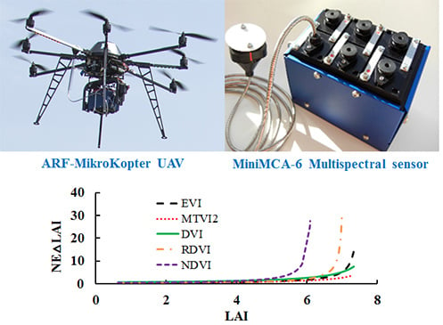
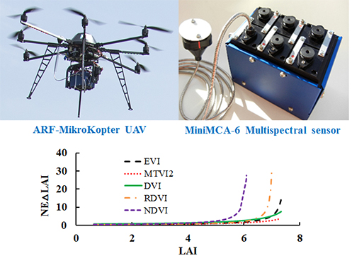
Other VIs, such as RDVI (800, 700), DVI (800, 700), NDVI (800,700), GNDVI (800, 550), RVI (800, 700), SAVI (800, 700), MSR (800, 700), EVI (490, 700, 800), and GBNDVI (490, 550, 800), also had better performance, but some of these had the limitation of saturation under the moderate-to-high LAI levels as often found in high-yielding wheat crops.

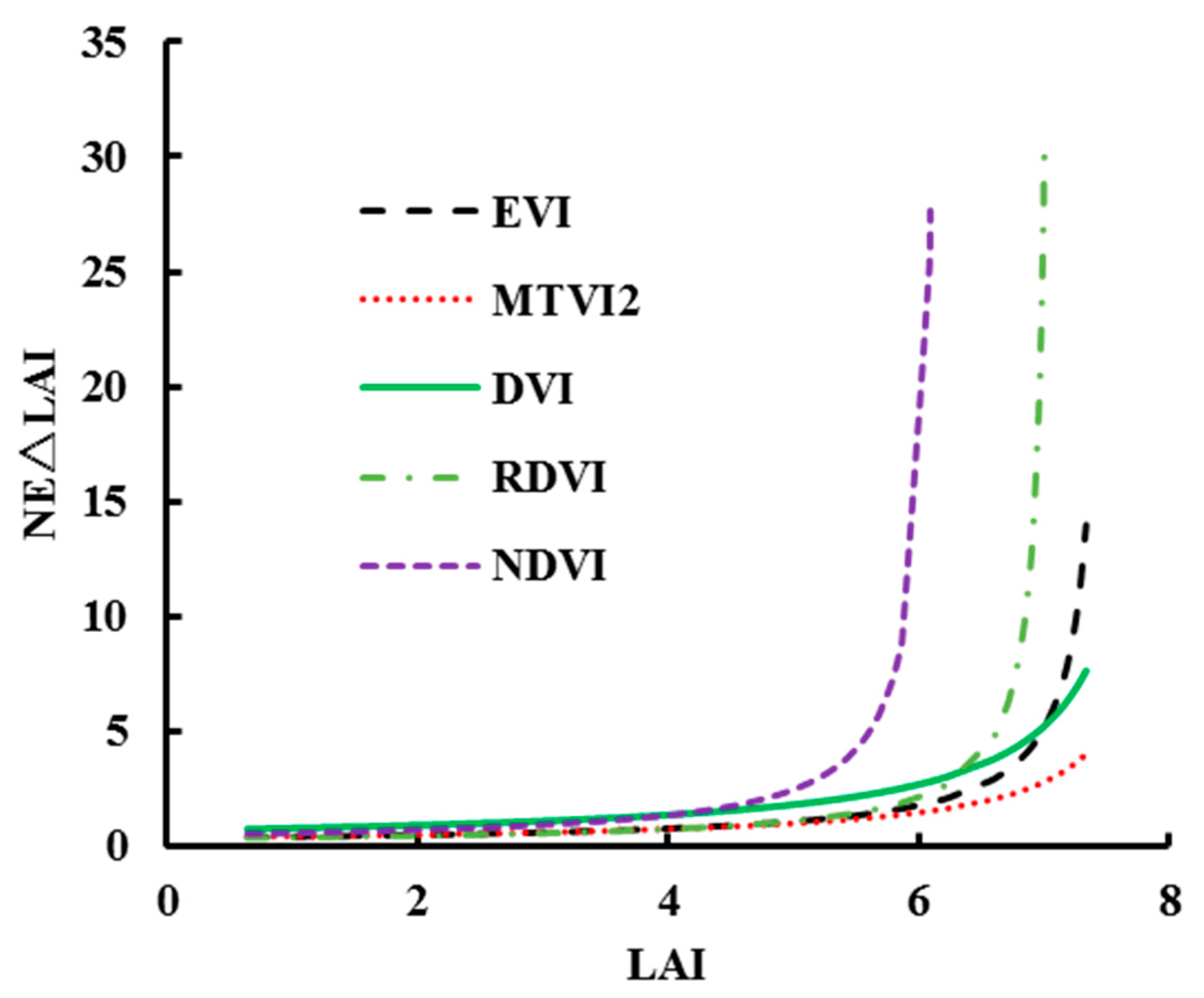
4.2. Saturation of VIs under Varied LAI Leves in Wheat

Saturation of VIs is one of the major limitations in estimating the biophysical parameters on the linear regression. Some previous studies demonstrated that NDVI was accurate and robust in LAI estimation for various vegetation types; however, NDVI is limited by the low accuracy related to saturation occurring in relatively dense canopies (LAI > 2 m² m⁻²) [50,51]. Smith, et al. [43] also showed that NDVI will demonstrate saturation status when the LAI reaches 3~4. And, the NDVI-derived model was underestimated during the grain filling period. Later, NDVI was proven to monitor the growth status on the canopy imagery by the UAVs, but serious saturation phenomenon appeared [14,15]. Hunt [52] also found that TGI (670, 480, 550) was not sensitive to changes in LAI > 2.0. Recently, a new index mNDSI (ρ940, 0.8ρ950, ρ730) which was more sensitive under the LAI conditions from 2 to 8 m² m⁻² was proposed from the author’s lab [51]. This paper did not specifically solve the saturation issue, but we fully assessed the saturation of those selected VI_S, and the result showed that the new model on MTVI₂ had higher sensitivity under different LAI ranges. What is more, the model could be applied in the LAI range of 2 to 7 m² m⁻², which would greatly enlarge the range of application compared to previous models.

4.3. Effect of LAI Estimation on the Application of the Methodology

The leaf area index is an important descriptor of many biological and physical processes of vegetation. Most of the currently available ground-based methods to estimate the LAI include either direct contact destructive sampling and point contact sampling, or indirect light transmittance (2000 Plant Canopy Analyzer) or spectral reflectance (Analytical Spectral Devices) methods. They are difficult to move from one site to another with a small-extent mapping capability. On the other hand, it appeared that satellite sensors did not meet the requirements in increasing image temporal frequency and spatial resolution for agricultural application like crop monitoring. However, remote sensing sensors placed on unmanned aerial vehicles represent a promising option to fill this gap, providing low-cost and high efficiency approaches to meet the critical requirements of spatial, spectral, and temporal resolutions.

Fortunately, in this research, we found that the LAI model with MTVI₂ has better accuracy with higher efficiency and lower error and is sensitive under various LAI values (from 2 to 7). Developing simple but efficient methods to monitor vegetation across a wide range of LAI is urgently needed for precision agriculture in China, where most of the field is with high LAI. In recent years, the application of nitrogen fertilizer increase year by year to meet the need of high production, which brings out the larger LAI than before. Therefore, the monitoring of LAI under medium and high level is important in practical production. In addition, the high cost of the equipment used here may be afforded by the owners of larger farms, or farmers associations that can share the benefits and also the costs, which is also important in China, since the farmer are not rich.

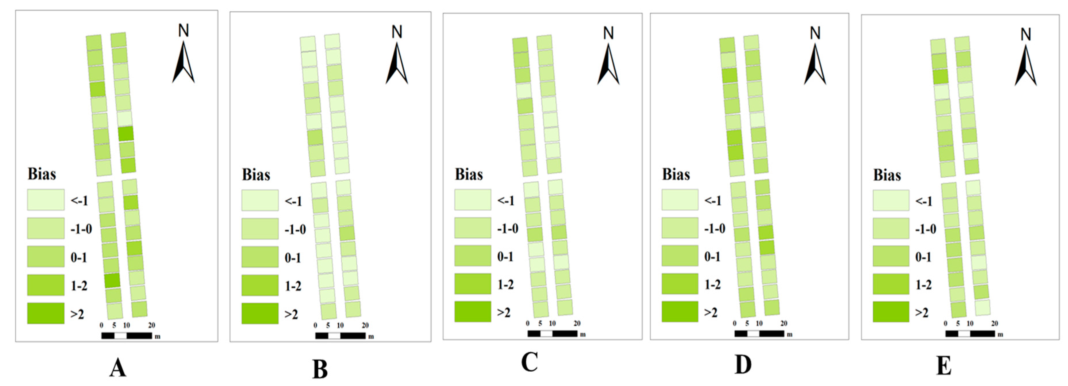
5. Conclusions

In this study, the major findings show that MTVI₂ (800, 700, 550) has the best performance in monitoring wheat LAI during the five critical growth stages, and the new developed LAI model demonstrated higher stability in the sub-strategies (including varied growth status) which could broaden the applied range (the maximum LAI reaches 7), when compared to the existing LAI model. The map of spatial distribution represents the dynamic change of wheat LAI, which shows relevant information for fertilizer practices. In summary, the UAVs technology is feasible in the monitoring of crop LAI for higher nitrogen nutrient fields at farm-scale in modern China. Accurate monitoring of wheat LAI is not only important in acquiring the growth status, but also provides crucial technical support to manage fertilizer applications for family farms. Previous studies have shown that critical N concentration curve on LAI can be an effective approach to diagnose the nutrient state and optimize N management in precision agriculture [53,54].

In practical use, a farm with the area of 5–10 ha could be fully covered with only 6–12 images at the flight altitude of 150 m. and the time will last an hour for the flight and pre-processing of imagery, which is high efficiency and low cost. However, there is still some work to be done to make the technology easy and simple, before we guide the addressing fertilization. It is still difficult to apply this technique to calculate the LAI for a general farmer, since not all the farmers can operate the UAV and pre-process image (vignette reduction, lens distortion correction, band registration, radiometric calibration and background removal), only if we could train them. So, we should develop a simple and easy LAI estimation software system on UAV_S in the future research. In addition, we should consider research on carrying hyperspectral sensors on UAVs to obtain important information, fully taking advantage of the textural information to enhance the accuracy, stability and universality of the model.

References

1. Gower, S.T.; Kucharik, C.J.; Norman, J.M. Direct and indirect estimation of leaf area index, f APAR, and net primary production of terrestrial ecosystems. Remote Sens. Environ. 1999, 70, 29–51. [Google Scholar] [CrossRef]
2. Laliberte, A.S.; Goforth, M.A.; Steele, C.M.; Rango, A. Multispectral remote sensing from unmanned aircraft: Image processing workflows and applications for rangeland environments. Remote Sens. 2011, 3, 2529–2551. [Google Scholar] [CrossRef]
3. Brisco, B.; Brown, R.J.; Hirose, T.; Mcnairn, H.; Staenz, K. Precision agriculture and the role of remote sensing: A review. Can. J. Remote Sens. 1998, 24, 315–327. [Google Scholar] [CrossRef]
4. Atzberger, C. Advances in remote sensing of agriculture: Context description, existing operational monitoring systems and major information needs. Remote Sens. 2013, 5, 949–981. [Google Scholar] [CrossRef]
5. Behrens, T.; Diepenbrock, W. Using digital image analysis to describe canopies of winter oilseed rape (Brassica napus L.) during vegetative developmental stages. J. Agron. Crop Sci. 2006, 192, 295–302. [Google Scholar] [CrossRef]
6. Liu, J.; Pattey, E.; Jégo, G. Assessment of vegetation indices for regional crop green LAI estimation from Landsat images over multiple growing seasons. Remote Sens. Environ. 2012, 123, 347–358. [Google Scholar] [CrossRef]
7. Zhang, Y.; Chen, J.M.; Miller, J.R.; Noland, T. Leaf chlorophyll content retrieval from airborne hyperspectral remote sensing imagery. Remote Sens. Environ. 2008, 112, 3234–3247. [Google Scholar] [CrossRef]
8. Von Bueren, S.; Burkart, A.; Hueni, A.; Rascher, U.; Tuohy, M.; Yule, I. Comparative validation of UAV based sensors for the use in vegetation monitoring. Biogeosci. Discuss. 2014, 11, 3837–3864. [Google Scholar] [CrossRef] [Green Version]
9. Lu, D.; Chen, Q.; Wang, G.; Moran, E.; Batistella, M.; Zhang, M.; Laurin, G.; Saah, D. Aboveground forest biomass estimation with Landsat and LiDAR data and uncertainty analysis of the estimates. Int. J. For. Res. 2012, 2012, 436537. [Google Scholar] [CrossRef]
10. Calderon, R.; Navas-Cortes, J.A.; Lucena, C.; Zarco-Tejada, P.J. High-resolution airborne hyperspectral and thermal imagery for early detection of Verticillium wilt of olive using fluorescence, temperature and narrow-band spectral indices. Remote Sens. Environ. 2013, 139, 231–245. [Google Scholar] [CrossRef]
11. Zhang, Q.; Su, Z.B.; Yang, G.J.; Wang, M.H.; Shen, W.Z.; Teng, X.W.; Dong, J.H. Intercomparison of ADC-Lite Images on UAV and TM Simulation Data for Soybean Leaf Area Index Retrieval. Int. J. Hybrid Inf. Technol. 2016, 9, 151–160. [Google Scholar] [CrossRef]
12. Chianucci, F.; Disperati, L.; Guzzic, D.; Bianchini, D.; Nardino, V.; Lastric, C.; Rindinell, A.; Coron, P. Estimation of canopy attributes in beech forests using true colour digital images from a small fixed-wing UAV. Int. J. Appl. Earth Obs. Geoinf. 2016, 47, 60–68. [Google Scholar] [CrossRef] [Green Version]
13. Delegido, J.; Verrelst, J.; Meza, C.M.; Rivera, J.P.; Alonso, L.; Moreno, J. A red-edge spectral index for remote sensing estimation of green LAI over agroecosystems. Eur. J. Agron. 2013, 46, 42–52. [Google Scholar] [CrossRef]
14. Hunt, E.R., Jr.; Hively, W.D.; Fujikawa, S.J.; Linden, D.S.; Daughtry, C.S.T.; Mccarty, G.W. Acquisition of NIR-green-blue digital photographs from unmanned aircraft for crop monitoring. Remote Sens. 2010, 2, 290–305. [Google Scholar] [CrossRef]
15. Lelong, C.C.; Burger, P.; Jubelin, G.; Roux, B.; Labbé, S.; Baret, F. Assessment of unmanned aerial vehicles imagery for quantitative monitoring of wheat crop in small plots. Sensors 2008, 8, 3557–3585. [Google Scholar] [CrossRef] [PubMed]
16. Torres-Sanchez, J.; Lopez-Granados, F.; De Castro, A.I.; Pena-Barragan, J.M. Configuration and Specifications of an Unmanned Aerial Vehicle (UAV) for Early Site Specific Weed Management. PLoS ONE 2013, 8, e58210. [Google Scholar] [CrossRef] [PubMed]
17. Hernández-Clemente, R.; Navarro-Cerrillo, R.M.; Zarco-Tejada, P.J. Carotenoid content estimation in a heterogeneous conifer forest using narrow-band indices and PROSPECT + DART simulations. Remote Sens. Environ. 2012, 127, 298–315. [Google Scholar] [CrossRef]
18. Jin, X.; Liu, S.; Baret, F.; Hemerlé, M.; Comar, A. Estimates of plant density of wheat crops at emergence from very low altitude UAV imagery. Remote Sens. Environ. 2017, 198, 105–114. [Google Scholar] [CrossRef]
19. Zhou, X.; Zheng, H.B.; Xu, X.Q.; He, J.Y.; Ge, X.K.; Yao, X.; Cheng, T.; Zhu, Y.; Cao, W.X.; Tian, Y.C. Predicting grain yield in rice using multi-temporal vegetation indices from UAV-based multispectral and digital imagery. ISPRS J. Photogramm. Remote Sens. 2017, 130, 246–255. [Google Scholar] [CrossRef]
20. Potgieter, A.B.; George-Jaeggli, B.; Chapman, S.C.; Laws, K.; Suárez Cadavid, L.A.; Wixted, J.; Wason, J.; Eldridge, M.; Jordan, D.R.; Hammer, G.L. Multi-spectral imaging from an unmanned aerial vehicle enables the assessment of seasonal leaf area dynamics of sorghum breeding lines. Front. Plant Sci. 2017, 8. [Google Scholar] [CrossRef] [PubMed]
21. Turner, D.P.; Cohen, W.B.; Kennedy, R.E.; Fassnacht, K.S.; Briggs, J.M. Relationships between leaf area index and Landsat TM spectral vegetation indices across three temperate zone sites. Remote Sens. Environ. 1999, 70, 52–68. [Google Scholar] [CrossRef]
22. Huete, A.; Didan, K.; Miura, T.; Rodriguez, E.P.; Gao, X.; Ferreira, L.G. Overview of the radiometric and biophysical performance of the MODIS vegetation indices. Remote Sens. Environ. 2002, 83, 195–213. [Google Scholar] [CrossRef]
23. Haboudane, D.; Miller, J.R.; Pattey, E.; Zarco-Tejada, P.J.; Strachan, I.B. Hyperspectral vegetation indices and novel algorithms for predicting green LAI of crop canopies: Modeling and validation in the context of precision agriculture. Remote Sens. Environ. 2004, 90, 337–352. [Google Scholar] [CrossRef]
24. Huete, A.R. A soil-adjusted vegetation index (SAVI). Remote Sens. Environ. 1988, 25, 295–309. [Google Scholar] [CrossRef]
25. Qi, J.; Chehbouni, A.; Huete, A.R.; Kerr, Y.H.; Sorooshian, S. A modified soil adjusted vegetation index. Remote Sens. Environ. 1994, 48, 119–126. [Google Scholar] [CrossRef]
26. Tian, W.; Xiao, R. Comparative study on the moderate scale of grain crop family farms in China. Hunan Agric. Sci. 2017, 8, 103–105. [Google Scholar]
27. McCabe, M.F.; Houborg, R.; Rosas, J. The potential of unmanned aerial vehicles for providing information on vegetation health. In Proceedings of the 21st International Congress on Modelling and Simulation, Gold Coast, Australia, 29 November–4 December 2015. [Google Scholar]
28. Kelcey, J.; Lucieer, A. Sensor correction of a 6-band multispectral imaging sensor for UAV remote sensing. Remote Sens. 2012, 4, 1462–1493. [Google Scholar] [CrossRef]
29. Wang, J.; Shi, F.; Zhang, J.; Liu, Y. A new calibration model and method of camera lens distortion. In Proceedings of the IEEE/RSJ International Conference on Intelligent Robots and Systems, Beijing, China, 9–15 October 2006; pp. 5713–5718. [Google Scholar]
30. Hugemann, W. Correcting Lens Distortions in Digital Photographs; Ingenieurbüro Morawski+ Hugemann: Leverkusen, Germany, 2010. [Google Scholar]
31. De Villiers, J.P.; Leuschner, F.W.; Geldenhuys, R. Modeling of radial asymmetry in lens distortion facilitated by modern optimization techniques. In Proceedings of the SPIE—The International Society for Optical Engineering, San Jose, CA, USA, 17–21 January 2010. [Google Scholar]
32. Turner, D.; Lucieer, A.; Malenovsky, Z.; King, D.H.; Robinson, S.A. Spatial co-registration of ultra-high resolution visible, multispectral and thermal images acquired with a micro-UAV over Antarctic moss beds. Remote Sens. 2014, 6, 4003–4024. [Google Scholar] [CrossRef]
33. Smith, G.M.; Milton, E.J. The use of the empirical line method to calibrate remotely sensed data to reflectance. Int. J. Remote Sens. 1999, 20, 2653–2662. [Google Scholar] [CrossRef]
34. Jia, X.; Richards, J.A. Segmented principal components transformation for efficient hyperspectral remote-sensing image display and classification. IEEE Trans. Geosci. Remote Sens. 1999, 37, 538–542. [Google Scholar]
35. Birth, G.S.; Mcvey, G.R. Measuring the color of growing turf with a reflectance spectrophotometer. Agrobiol. J. 1968, 60, 640–643. [Google Scholar] [CrossRef]
36. Rouse, J.W. Monitoring the Vernal Advancement and Retrogradation (Green Wave Effect) of Natural Vegetation; NASA/GSFCT Type III Final Report; National Aeronautics and Space Administration (NASA): Washington, DC, USA, 1974.
37. Wang, F.M.; Huang, J.F.; Tang, Y.L.; Wang, X.Z. New vegetation index and its application in estimating leaf area index of rice. Rice Sci. 2007, 14, 195–203. [Google Scholar] [CrossRef]
38. Broge, N.H.; Leblanc, E. Comparing prediction power and stability of broadband and hyperspectral vegetation indices for estimation of green leaf area index and canopy chlorophyll density. Remote Sens. Environ. 2001, 76, 156–172. [Google Scholar] [CrossRef]
39. Gitelson, A.A.; Kaufman, Y.J.; Merzlyak, M.N. Use of a green channel in remote sensing of global vegetation from EOS-MODIS. Remote Sens. Environ. 1996, 58, 289–298. [Google Scholar] [CrossRef]
40. Chen, J.M.; Cihlar, J. Retrieving leaf area index of boreal conifer forests using Landsat TM images. Remote Sens. Environ. 1996, 55, 153–162. [Google Scholar] [CrossRef]
41. Jordan, C.F. Derivation of leaf-area index from quality of light on the forest floor. Ecology 1969, 50, 663–666. [Google Scholar] [CrossRef]
42. Gitelson, A. Remote estimation of crop fractional vegetation cover: The use of noise equivalent as an indicator of performance of vegetation indices. Int. J. Remote Sens. 2013, 34, 6054–6066. [Google Scholar] [CrossRef]
43. Smith, A.M.; Bourgeois, G.; Teillet, P.M.; Freemantle, J.; Nadeau, C. A comparison of NDVI and MTVI2 for estimating LAI using CHRIS imagery: A case study in wheat. Can. J. Remote Sens. 2008, 34, 539–548. [Google Scholar] [CrossRef]
44. Herrmann, I.; Pimstein, A.; Karnieli, A.; Cohen, Y.; Alchanatis, V.; Bonfil, D.J. LAI assessment of wheat and potato crops by VENμS and Sentinel-2 bands. Remote Sens. Environ. 2011, 115, 2141–2151. [Google Scholar] [CrossRef]
45. Main, R.; Cho, M.A.; Mathieu, R.; O’Kennedy, M.M.; Ramoelo, A.; Koch, S. An investigation into robust spectral indices for leaf chlorophyll estimation. ISPRS J. Photogramm. Remote Sens. 2011, 66, 751–761. [Google Scholar] [CrossRef]
46. Clevers, J.G.P.W.; Gitelson, A.A. Remote estimation of crop and grass chlorophyll and nitrogen content using red-edge bands on Sentinel-2 and -3. Int. J. Appl. Earth Obs. Geoinf. 2013, 23, 344–351. [Google Scholar] [CrossRef]
47. Gitelson, A.; Merzlyak, M.N. Quantitative estimation of chlorophyll-a using reflectance spectra: Experiments with autumn chestnut and maple leaves. J. Photochem. Photobiol. B Biol. 1994, 22, 247–252. [Google Scholar] [CrossRef]
48. Nguy-Robertson, A.L.; Peng, Y.; Gitelson, A.A.; Arkebauer, T.J.; Pimstein, A.; Herrmann, I.; Karnieli, A.; Rundquist, D.C.; Bonfil, D.J. Estimating green LAI in four crops: Potential of determining optimal spectral bands for a universal algorithm. Agric. For. Meteorol. 2014, 192–193, 140–148. [Google Scholar] [CrossRef]
49. Rodriguezperez, J.R.; Riano, D.; Carlisle, E.; Ustin, S.; Smart, D.R. Evaluation of hyperspectral reflectance indexes to detect grapevine water status in vineyards. Am. J. Enol. Vitic. 2007, 58, 302–317. [Google Scholar]
50. Gitelson, A. A Wide dynamic range vegetation index for remote quantification of biophysical characteristics of vegetation. J. Plant Physiol. 2004, 161, 165–173. [Google Scholar] [CrossRef] [PubMed]
51. Cao, Z.; Cheng, T.; Ma, X.; Tian, Y.; Zhu, Y.; Yao, X.; Chen, Q.; Liu, S.; Guo, Z.; Zhen, Q.; et al. A new three-band spectral index for mitigating the saturation in the estimation of leaf area index in wheat. Int. J. Remote Sens. 2017, 38, 3865–3885. [Google Scholar] [CrossRef]
52. Hunt, E.R.; Doraiswamy, P.C.; McMurtrey, J.E.; Daughtry, C.S.T.; Perry, E.M.; Akhmedov, B. A visible band index for remote sensing leaf chlorophyll content at the canopy scale. Int. J. Appl. Earth Obs. Geoinf. 2013, 21, 103–112. [Google Scholar] [CrossRef]
53. Plénet, D.; Lemaire, G. Relationships between dynamics of nitrogen uptake and dry matter accumulation in maize crops. Determination of critical N concentration. Plant Soil 1999, 216, 65–82. [Google Scholar] [CrossRef]
54. Ata-Ul-Karim, S.T.; Zhu, Y.; Yao, X.; Cao, W.X. Determination of critical nitrogen dilution curve based on leaf area index in rice. Field Crops Res. 2014, 167, 76–85. [Google Scholar] [CrossRef]
Figure 1. The UAV imagery with two winter wheat varieties (V1, V2), two densities (D1, D2), three nitrogen rates (N0, N1, N2) (A), location of our field pilot trial with 36 plots (B).
Remotesensing 09 01304 g001
Figure 2. The UAV and sensor (A) Graupner MC-32, (B) ARF-MikroKopter UAV, (C) Multispectral sensor, (D) Ground control point.
Remotesensing 09 01304 g002
Figure 3. Canopy spectral reflectance of the narrowband multispectral image at various growth stages and days after sowing (DAS). (a) jointing stage, DAS = 133; (b) booting stage, DAS = 158; (c) heading stage, DAS = 166; (d) anthesis stage, DAS = 173; (e) grain filling stage, DAS = 186; (f) the five critical growth stages.
Remotesensing 09 01304 g003
Figure 4. Saturation sensitivity of selected VIS to LAI.
Remotesensing 09 01304 g004
Figure 5. Bias mapping of LAI between measured and predicted values. (A) Jointing stage, (B) Booting stage, (C) Heading stage, (D) Anthesis stage, (E) Grain filling stage.
Remotesensing 09 01304 g005