A Novel Approach to the Identification of Compromised Pulmonary Systems in Smokers by Exploiting Tidal Breathing Patterns

 ,
,
Abstract
:1. Introduction
2. Related Work
2.1. TBA: A Physiological Modality of Pulmonary Artifact Detection
2.2. TBA of Compromised Adult Lungs: The Paradigm Shift
2.3. Tidal Breathing Data Acquisition Techniques
3. Methodology
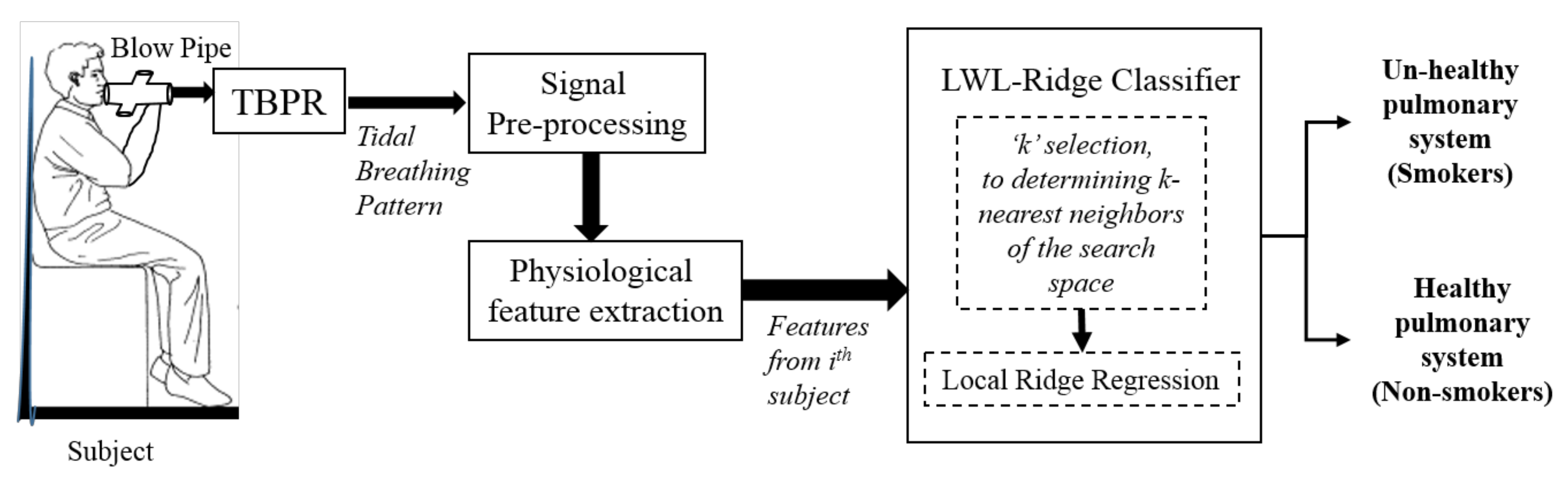
3.1. Overall System
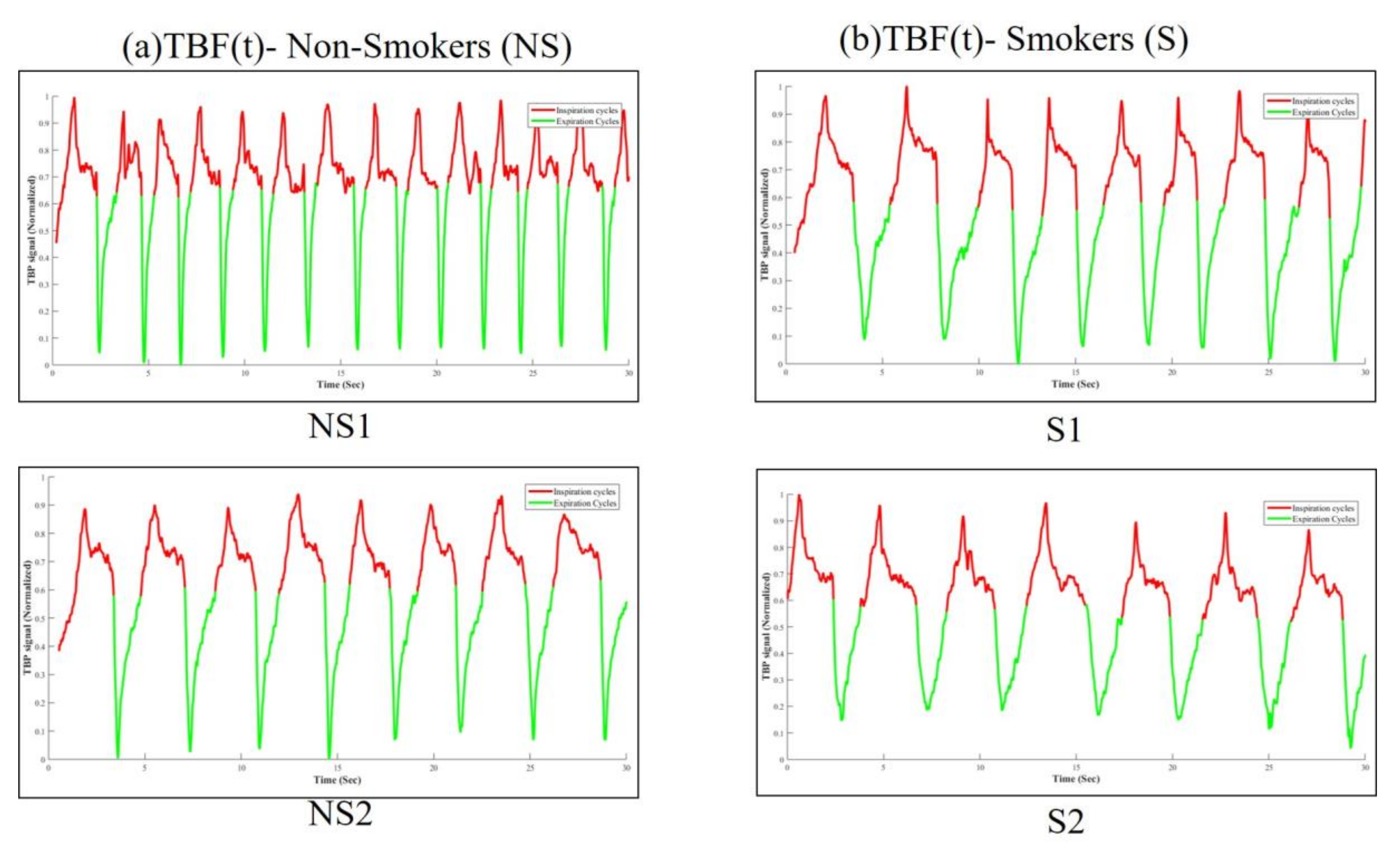
3.2. Tidal Breathing Pattern Acquisition
3.3. Experimental Setup
3.4. Signal Preprocessing and Feature Extraction
3.5. Classification Model
4. Results and Discussion
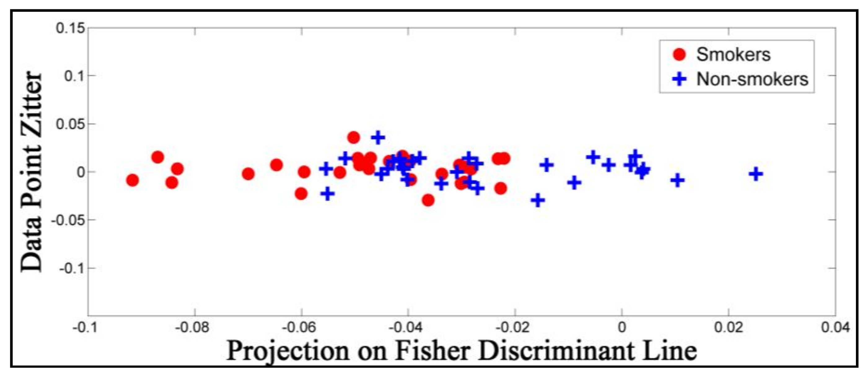
4.1. Feature Level Discriminability
4.2. Selection of Ridge Regression for LWL
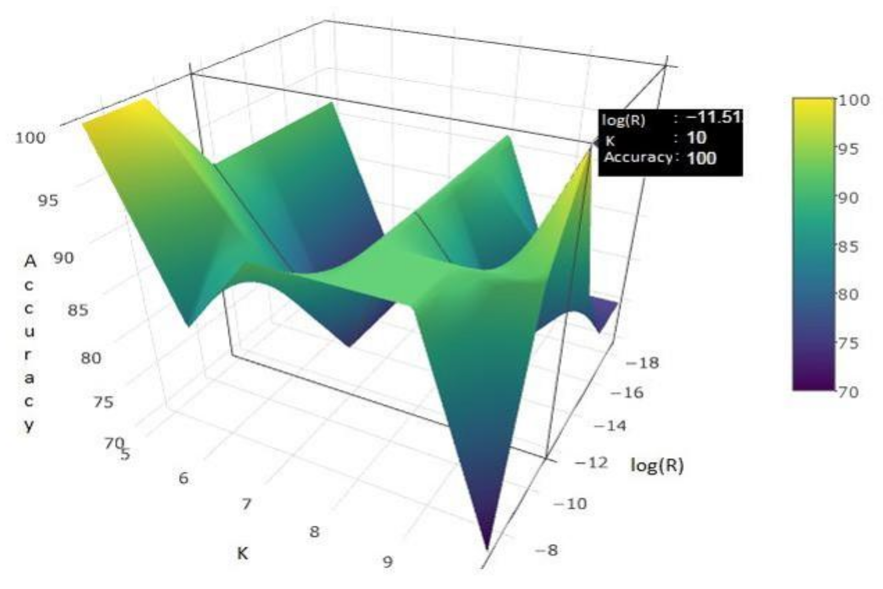
4.3. Determination of LWL-Ridge Parameters: K and R
4.4. Performance of Chosen Tuned Model on Simulated Dataset
4.5. Statistical Test
4.6. Evaluation of System Performance on an External Cohort
4.7. Comparison with Relevant State-of-the-Art
- TTOT = Total time of one complete breathing cycle = TI +TE
- TPTEF/TE = Ratio of TPTEF to TE
- TPTIF/TI = Ratio of TPTIF to TI
- VT = Tidal volume = TVins + TVexp
- VT/TI = Ratio of tidal volume to inspiratory time
- IP PEF = Integral of expiratory signal from peak to end.
- TP PEF20(80) = Post-peak expiratory flow at time 20%(80%).
- VE = Minute ventilation. Volume of air breathed per minute.
5. Conclusions
Author Contributions
Conflicts of Interest
References
- Hurd, S. The impact of COPD on lung health worldwide: Epidemiology and incidence. Chest J. 2000, 117, 1S–4S. [Google Scholar] [CrossRef]
- Chronic Obstructive Pulmonary Disease (COPD). Available online: http://www.who.int/mediacentre/factsheets/fs315/en/ (accessed on 19 August 2017).
- Estimated Incidence, Mortality and Prevalence Worldwide in 2012. Available online: http://globocan.iarc.fr/Pages/fact sheets cancer.aspx (accessed on 19 August 2017).
- Miller, M.R.; Hankinson, J.A.T.S.; Brusasco, V.; Burgos, F.; Casaburi, R.; Coates, A.; Crapo, R.; Enright, P.V.; van der Grinten, C.P.M.; Gustafsson, P.; et al. Standardisation of spirometry. Eur. Respir. J. 2005, 26, 319–338. [Google Scholar] [CrossRef] [PubMed]
- Khasnobish, A.; Rakshit, R.; Sinharay, A.; Chakravarty, T. Phase-gain IC based novel design of tidal breathing pattern sensor for pulmonary disease diagnostics: Demo abstract. In Proceedings of the 16th ACM/IEEE International Conference on Information Processing in Sensor Networks, Pittsburgh, PA, USA, 18–21 April 2017; pp. 273–274. [Google Scholar]
- Sinharay, A.; Rakshit, R.; Khasnobish, A.; Ghosh, D.; Pal, A.; Chakravrty, T. The Ultrasonic Directional Tidal Breathing Pattern Sensor: Equitable Design Realization Based on Phase Information. Sensors 2017, 17, 1853. [Google Scholar] [CrossRef] [PubMed]
- Proctor, R.N. The history of the discovery of the cigarette-lung cancer link: Evidentiary traditions, corporate denial, global toll. Tob. Control 2012, 21, 87–91. [Google Scholar] [CrossRef] [PubMed]
- Sawyer, K.C.; Sawyer, R.B.; Lubchenco, A.E.; McKinnon, D.A.; Hill, K.A. Fatal primary cancer of the lung in a teen-age smoker. Cancer 1967, 20, 451–457. [Google Scholar] [CrossRef]
- Fletcher, C.; Peto, R. The natural history of chronic airflow obstruction. Br. Med. J. 1977, 1, 1645–1648. [Google Scholar] [CrossRef] [PubMed]
- Maury, B. The Respiratory System in Equations; Springer: Milan, Italy, 2013. [Google Scholar]
- Sharma, G.; Goodwin, J. Effect of aging on respiratory system physiology and immunology. Clin. Interventions Aging 2006, 1, 253–260. [Google Scholar] [CrossRef]
- Chhabra, S.K. Regional variations in vital capacity in adult males in India: Comparison of regression equations from four regions and impact on interpretation of spirometric data. Indian J. Chest Dis. Allied Sci. 2009, 51, 7. [Google Scholar] [PubMed]
- Bhatti, U.; Rani, K.; Memon, M.Q. Variation in lung volumes and capacities among young males in relation to height. J. Ayub Med. Coll. Abbottabad 2014, 26, 200–202. [Google Scholar] [PubMed]
- Mead, J.; Whittenberger, J.L. Physical properties of human lungs measured during spontaneous respiration. J. Appl. Physiol. 1953, 5, 779–796. [Google Scholar] [CrossRef]
- Williams, E.; Powell, T.; Eriksen, M.; Neill, P.; Colasanti, R. A pilot study quantifying the shape of tidal breathing waveforms using centroids in health and COPD. J. Clin. Monit. Comput. 2014, 28, 67–74. [Google Scholar] [CrossRef] [PubMed]
- Ma, S.; Hecht, A.; Varga, J.; Rambod, M.; Morford, S.; Goto, S.; Casaburi, R.; Porszasz, J. Breath-by-breath quantification of progressive airflow limitation during exercise in COPD: A new method. Respir. Med. 2010, 104, 389–396. [Google Scholar] [CrossRef] [PubMed]
- Colasanti, R.L.; Morris, M.J.; Madgwick, R.G.; Sutton, L.; Williams, E.M. Analysis of tidal breathing profiles in cystic fibrosis and COPD. Chest 2004, 125, 901–908. [Google Scholar] [CrossRef] [PubMed]
- Satoh, D.; Kurosawa, S.; Kirino, W.; Wagatsuma, T.; Ejima, Y.; Yoshida, A.; Toyama, H.; Nagaya, K. Impact of changes of positive end-expiratory pressure on functional residual capacity at low tidal volume ventilation during general anesthesia. J. Anesth. 2012, 26, 664–669. [Google Scholar] [CrossRef] [PubMed]
- Halbertsma, F.J.; Vaneker, M.; Pickkers, P.; Hoeven, J.G. The oxygenation ratio during mechanical ventilation in children: The role of tidal volume and positive end-expiratory pressure. J. Crit. Care 2009, 24, 220–226. [Google Scholar] [CrossRef] [PubMed]
- Imanaka, H.; Takeuchi, M.; Tachibana, K.; Nishimura, M. Expiratory tidal volume displayed on bird 8400STi can exceed the preset tidal volume due to cardiogenic oscillation: A lung model study. J. Anesth. 2004, 18, 313–315. [Google Scholar] [CrossRef] [PubMed]
- Morris, D.J.; Lane, M.J. Tidal expiratory flow patterns in airflow obstruction. Thorax 1981, 36, 135–142. [Google Scholar] [CrossRef] [PubMed]
- Van der Ent, C.; Brackel, H.; van der Laag, J.; Bogaard, J.M. Tidal breathing analysis as a measure of airway obstruction in children three years of age and older. Am. J. Respir. Crit. Care Med. 1996, 153, 1253–1258. [Google Scholar] [CrossRef] [PubMed]
- Bates, J.; Schmalisch, G.; Filbrun, D.; Stocks, J. Tidal breath analysis for infant pulmonary function testing. ERS/ATS task force on standards for infant respiratory function testing. European respiratory society/american thoracic society. Eur. Respir. J. 2000, 16, 1180–1192. [Google Scholar] [CrossRef] [PubMed]
- Frey, U.; Stocks, J.; Coates, A.; Sly, P.; Bates, J. Specifications for equipment used for infant pulmonary function testing. ers/ats task force on standards for infant respiratory function testing. European respiratory society/american thoracic society. Eur. Respir. J. 2000, 16, 731–740. [Google Scholar] [CrossRef] [PubMed]
- Frey, U.; Stocks, J.; Sly, P.; Bates, J. Specification for signal processing and data handling used for infant pulmonary function testing. ERS/ATS task force on standards for infant respiratory function testing. European respiratory society/american thoracic society. Eur. Respir. J. 2000, 16, 1016–1022. [Google Scholar] [CrossRef] [PubMed]
- Zheng, C.-J.; Adams, A.B.; McGrail, M.P.; Marini, J.J.; Greaves, I.A. A proposed curvilinearity index for quantifying airflow obstruction. Respir. Care 2006, 51, 40–45. [Google Scholar] [CrossRef] [PubMed]
- Wildhaber, J.H.; Sznitman, J.; Harpes, P.; Straub, D.; Möller, A.; Basek, P.; Sennhauser, F.H. Correlation of spirometry and symptom scores in childhood asthma and the usefulness of curvature assessment in expiratory flow-volume curves. Respir. Care 2007, 52, 1744–1752. [Google Scholar] [PubMed]
- Weintraub, Z.; Cates, D.; Kwiatkowski, K.; Al-Hathlol, K.; Hussain, A.; Rigatto, H. The morphology of periodic breathing in infants and adults. Respir. Physiol. 2001, 127, 173–184. [Google Scholar] [CrossRef]
- Habib, R.H.; Pyon, K.H.; Courtney, S.E.; Aghai, Z.H. Spectral characteristics of airway opening and chest wall tidal flows in spontaneously breathing preterm infants. J. Appl. Physiol. 2003, 94, 1933–1940. [Google Scholar] [CrossRef] [PubMed]
- Leonhardt, S.; Kecman, V. Novel features for automated lung function diagnosis in spontaneously breathing infants. In Proceedings of the Conference on Artificial Intelligence in Medicine in Europe, Amsterdam, The Netherlands, 7–11 July 2007; Springer: Berlin/Heidelberg, Germany, 2007; pp. 195–199. [Google Scholar]
- Leonhardt, S.; Ahrens, P.; Kecman, V. Analysis of tidal breathing flow volume loops for automated lung-function diagnosis in infants. IEEE Trans. Biomed. Eng. 2010, 57, 1945–1953. [Google Scholar] [CrossRef] [PubMed]
- Beydon, N.; Davis, S.D.; Lombardi, E.; Allen, J.L.; Arets, H.G.; Aurora, P.; Bisgaard, H.; Davis, G.M.; Ducharme, F.M.; Eigen, H.; et al. An official american thoracic society/european respiratory society statement: Pulmonary function testing in preschool children. Am. J. Respir. Crit. Care Med. 2007, 175, 1304–1345. [Google Scholar] [CrossRef] [PubMed]
- Milic-Emili, J. Does mechanical injury of the peripheral airways play a role in the genesis of COPD in smokers? COPD J. Chronic Obstr. Pulm. Dis. 2004, 1, 85–92. [Google Scholar] [CrossRef] [PubMed]
- Koulouris, N.; Hardavella, G. Physiological techniques for detecting expiratory flow limitation during tidal breathing. Eur. Respir. Rev. 2011, 20, 147–155. [Google Scholar] [CrossRef] [PubMed]
- Chiari, S.; Bassini, S.; Braghini, A.; Corda, L.; Boni, E.; Tantucci, C. Tidal expiratory flow limitation at rest as a functional marker of pulmonary emphysema in moderate-to-severe COPD. COPD J. Chronic Obstr. Pulm. Dis. 2014, 11, 33–38. [Google Scholar] [CrossRef] [PubMed]
- Sancho, J.; Servera, E.; Díaz, J.; Marín, J. Comparison of peak cough flows measured by pneumotachograph and a portable peak flow meter. Am. J. Phys. Med. Rehabil. 2004, 83, 608–612. [Google Scholar] [CrossRef] [PubMed]
- Marsh, M.J.; Ingram, D.; Milner, A.D. The effect of instrumental dead space on measurement of breathing pattern and pulmonary mechanics in the newborn. Pediatric Pulmonol. 1993, 16, 316–322. [Google Scholar] [CrossRef]
- Schmalisch, G.; Foitzik, B.; Wauer, R.; Stocks, J. Effect of apparatus dead space on breathing parameters in newborns: Flow-through versus conventional techniques. Eur. Respir. J. 2001, 17, 108–114. [Google Scholar] [CrossRef] [PubMed]
- Pearsall, M.F.; Feldman, J.M. When does apparatus dead space matter for the pediatric patient? Anesth. Analg. 2014. Reprint. [Google Scholar] [CrossRef] [PubMed]
- Schibler, A.; Henning, R. Measurement of functional residual capacity in rabbits and children using an ultrasonic flow meter. Pediatr. Res. 2001, 49, 581–588. [Google Scholar] [CrossRef] [PubMed]
- Buess, C.; Pietsch, P.; Guggenbuhl, W.; Koller, E. A pulsed diagonal-beam ultrasonic airflow meter. J. Appl. Physiol. 1986, 61, 1195–1199. [Google Scholar] [CrossRef] [PubMed]
- Konno, K.; Mead, J. Measurement of the separate volume changes of rib cage and abdomen during breathing. J. Appl. Physiol. 1967, 22, 407–422. [Google Scholar] [CrossRef] [PubMed]
- Vegfors, M.; Lindberg, L.G.; Pettersson, H.; Oberg, P.A. Presentation and evaluation of a new optical sensor for respiratory rate monitoring. Int. J. Clin. Monit. Comput. 1994, 11, 151–156. [Google Scholar] [CrossRef] [PubMed]
- Wolf, G.K.; Arnold, J.H. Electrical impedance tomography: Ready for prime time? Intensive Care Med. 2006, 32, 1290–1292. [Google Scholar] [CrossRef] [PubMed]
- Frerichs, I.; Braun, P.; Dudykevych, T.; Hahn, G.; Genée, D.; Hellige, G. Distribution of ventilation in young and elderly adults determined by electrical impedance tomography. Respir. Physiol. Neurobiol. 2004, 143, 63–75. [Google Scholar] [CrossRef] [PubMed]
- Hampshire, A.; Smallwood, R.; Brown, B.; Primhak, R. Multifrequency and parametric EIT images of neonatal lungs. Physiol. Meas. 1995, 16, A175. [Google Scholar] [CrossRef] [PubMed]
- WMA Declaration of Helsinki—Ethical Principles for Medical Research Involving Human Subjects. Available online: https://www.wma.net/policies-post/wma-declaration-of-helsinki-ethical-principles-for-medical-research-involving-human-subjects/ (accessed on 29 March 2018).
- Ding, X.; Yang, Y.; Stein, E.A.; Ross, T.J. Multivariate classification of smokers and nonsmokers using SVM-RFE on structural MRI images. Hum. Brain Mapp. 2015, 36, 4869–4879. [Google Scholar] [CrossRef] [PubMed]
- Cleveland, W.S. Robust locally weighted regression and smoothing scatterplots. J. Am. Stat. Assoc. 1979, 74, 829–836. [Google Scholar] [CrossRef]
- Le Cessie, S.; van Houwelingen, J.C. Ridge estimators in logistic regression. Appl. Stat. 1992, 41, 191–201. [Google Scholar] [CrossRef]
- Mahajan, V.; Jain, A.K.; Bergier, M. Parameter estimation in marketing models in the presence of multicollinearity: An application of ridge regression. J. Mark. Res. 1977, 14, 586–591. [Google Scholar] [CrossRef]
- Mika, S.; Ratsch, G.; Weston, J.; Scholkopf, B.; Mullers, K. Fisher discriminant analysis with kernels. In Proceedings of the 1999 IEEE Signal Processing Society Workshop Neural Networks for Signal Processing IX, Madison, WI, USA, 25 August 1999; pp. 41–48. [Google Scholar]
- Hall, M.; Frank, E.; Holmes, G.; Pfahringer, B.; Reutemann, P.; Witten, I.H. The WEKA data mining software: An update. ACM SIGKDD Explor. Newsl. 2009, 11, 10–18. [Google Scholar] [CrossRef]
- Fawcett, T. An introduction to ROC analysis. Pattern Recogn. Lett. 2006, 27, 861–874. [Google Scholar] [CrossRef]
- Duda, R.O.; Hart, P.E.; Stork, D.G. Pattern Classification; John Wiley & Sons: Hoboken, NJ, USA, 2012. [Google Scholar]
- Chawla, N.V.; Bowyer, K.W.; Hall, L.O.; Kegelmeyer, W.P. SMOTE: Synthetic minority over-sampling technique. J. Artif. Intell. Res. 2002, 16, 321–357. [Google Scholar]
- Schölkopf, B.; Burges, C.J.C.; Smola, A.J. (Eds.) Advances in Kernel Methods: Support Vector Learning; MIT Press: Cambridge, MA, USA, 1999. [Google Scholar]
- Breiman, L. Random forests. Mach. Learn. 2001, 45, 5–32. [Google Scholar] [CrossRef]
- Aha, D.W.; Kibler, D.; Albert, M.K. Instance-based learning algorithms. Mach. Learn. 1991, 6, 37–66. [Google Scholar] [CrossRef]
- Demšar, J. Statistical comparisons of classifiers over multiple data sets. J. Mach. Learn. Res. 2006, 7, 1–30. [Google Scholar]
- Hamblin, D.; Almirall, J. Analysis of exhaled breath from cigarette smokers using CMV-GC/MS. Forensic Chem. 2017, 4, 67–74. [Google Scholar] [CrossRef]
- Valencia, S.; Smith, M.V.; Atyabi, A.; Shic, F. Mobile ascertainment of smoking status through breath: A machine learning approach. In Proceedings of the IEEE Annual Ubiquitous Computing, Electronics & Mobile Communication Conference (UEMCON), New York, NY, USA, 20–22 October 2016; pp. 1–7. [Google Scholar]
- Witt, K.; Reulecke, S.; Voss, A. Discrimination and characterization of breath from smokers and non-smokers via electronic nose and GC/MS analysis. In Proceedings of the 2011 Annual International Conference of the IEEE Engineering in Medicine and Biology Society, EMBC, Boston, MA, USA, 30 August–3 September 2011; pp. 3664–3667. [Google Scholar]
- Garey, K.W.; Neuhauser, M.M.; Robbins, R.A.; Danziger, L.H.; Rubinstein, I. Markers of inflammation in exhaled breath condensate of young healthy smokers. Chest J. 2004, 125, 22–26. [Google Scholar] [CrossRef]


| Demographic Variable | Cohort 1 | Cohort 2 | ||
|---|---|---|---|---|
| Smokers | Non-Smokers | Smokers | Non-Smokers | |
| Number | 10 | 10 | 10 | 10 |
| Age | 35.3 ± 7.96 | 34.7 ± 6.32 | 29 ± 7.08 | 30 ± 7.07 |
| Gender | 8 M/2 F | 6 M/4 F | 9 M/1 F | 4 M/6 F |
| Smoking Years | 15.5 ± 6.86 | - | 13.4 ± 3.04 | - |
| CPD | 16.3 ± 4.74 | - | 14.6 ± 1.94 | - |
| Lifetime-Usage | 13.61 ± 9.63 | - | 10.06 ± 3.12 | - |
| Feature No. | Features | Description |
|---|---|---|
| F1 | Inspiratory time (TI) | Mean duration of all the acquired Inspiration phases in seconds |
| F2 | Expiratory time (TE) | Mean duration of all the acquired Expiration phases in seconds |
| F3 | Breathing rate (BR) | Number of breaths per minute |
| F4 | Duty Cycle (DCy) | Mean of the ratios of inspiration time to total breath time of all the acquired breath cycles |
| F5 | Peak Inspiratory Flow (PIF) | Maximum flow rate attained during the inspiratory period. |
| F6 | Peak Expiratory Flow (PEF) | Maximum flow rate attained during the expiratory period. |
| F7 | Time to Peak Inspiratory Flow (TP IF) | Mean time from onset to peak of inspiration of all inspiratory phases. |
| F8 | Time to Peak Expiratory Flow (TP EF) | Mean time from onset to peak of expiration of all expiratory phases. |
| F9 | Inspiratory Tidal volume (TVins) | Mean volume of air inspired of all the acquired inspiration phases |
| F10 | Expiratory Tidal volume (TVexp) | Mean volume of air expired of all the acquired expiration phases |
| F11 | Inspiratory velocity (Velins) | Mean velocity of inspiration from onset to peak of inspiration flow of all the acquired inspiration phases |
| F12 | Expiratory velocity (Velexp) | Mean velocity of expiration from onset to peak of expiration flow of all the acquired expiration phases |
| Scheme | % Acc | TPR | TNR | F | Kappa | AUC | AUP |
|---|---|---|---|---|---|---|---|
| LWL + L-R | 85.0 (18.07) | 0.80 (0.3) | 0.90 (0.09) | 0.70 (0.36) | 0.93 (0.09) | 0.92 (0.10) | 0.92 (0.11) |
| LWL + L-O | 80.83 (11.57) | 0.82 (0.15) | 0.80 (0.18) | 0.81 (0.11) | 0.62 (0.23) | 0.85 (0.13) | 0.86 (0.13) |
| L-R | 64.00 (13.41) | 0.60 (0.22) | 0.68 (0.16) | 0.61 (0.17) | 0.28 (0.27) | 0.69 (0.15) | 0.73 (0.12) |
| L-O | 63.83 (12.33) | 0.58 (0.22) | 0.70 (0.16) | 0.60 (0.18) | 0.28 (0.25) | 0.67 (0.14) | 0.72 (0.13) |
| Choices of {k, R} | T = 1/t of the Total Instances | ||||
|---|---|---|---|---|---|
| (i.e., 60 × 1/t) and t ∈ {2, 3, …, 7} | |||||
| 1/3 | 1/4 | 1/5 | 1/6 | 1/7 | |
| {10, 10−5} | 65 | 73.33 | 100 | 50 | 88.89 |
| {5, 10−4} | 85 | 80 | 100 | 70 | 88.89 |
| {5, 10−3} | 85 | 80 | 100 | 70 | 88.89 |
| R | % Acc | TPR | TNR | F | Kappa | AUC | AUP |
|---|---|---|---|---|---|---|---|
| 10−3 | 86.17 (10.46) | 0.84 (0.17) | 0.88 (0.14) | 0.85 (0.12) | 0.72 (0.21) | 0.92 (0.10) | 0.93 (0.10) |
| 10−4 | 85.02 (18.07) | 0.80 (0.3) | 0.90 (0.09) | 0.82 (0.24) | 0.70 (0.36) | 0.93 (0.09) | 0.90 (0.13) |
| No. of Instances (Actual + Simulated) | % Acc | TPR | TNR | Kappa | AUC | AUP |
|---|---|---|---|---|---|---|
| 60 + 60 | 94.08 (3.87) | 0.96 (0.05) | 0.92 (0.07) | 0.88 (0.08) | 0.97 (0.04) | 0.96 (0.06) |
| 60 + 120 | 93.22 (3.37) | 0.97 (0.04) | 0.90 (0.07) | 0.86 (0.07) | 0.96 (0.03) | 0.95 (0.05) |
| 60 + 180 | 95.12 (3.38) | 0.97 (0.03) | 0.94 (0.05) | 0.90 (0.07) | 0.98 (0.02) | 0.98 (0.03) |
| 60 + 240 | 95.87 (3.02) | 0.98 (0.02) | 0.94 (0.05) | 0.92 (0.06) | 0.99 (0.01) | 0.99 (0.02) |
| 60 + 300 | 95.44 (2.65) | 0.95 (0.03) | 0.95 (0.03) | 0.91 (0.05) | 0.98 (0.02) | 0.98 (0.02) |
| 60 + 360 | 97.64 (1.64) | 0.98 (0.02) | 0.97 (0.02) | 0.95 (0.03) | 1.00 (0.01) | 1.00 (0.01) |
| 60 + 420 | 96.04 (1.91) | 0.97 (0.03) | 0.96 (0.03) | 0.92 (0.04) | 0.99 (0.01) | 0.98 (0.02) |
| 60 + 480 | 96.56 (1.80) | 0.97 (0.03) | 0.96 (0.03) | 0.93 (0.04) | 0.99 (0.01) | 0.99 (0.01) |
| 60 + 540 | 96.40 (1.48) | 0.98 (0.02) | 0.95 (0.02) | 0.93 (0.03) | 0.99 (0.01) | 0.98 (0.02) |
| Method | % Acc | TPR | TNR | F | Kappa | AUC | AUP | Rank (Rj) |
|---|---|---|---|---|---|---|---|---|
| SVM-RBF | 51.67 | 0.67 | 0.37 | 0.55 | 0.03 | 0.52 | 0.51 | 4 |
| RF | 78.33 | 0.77 | 0.30 | 0.76 | 0.57 | 0.77 | 0.79 | 2.5 |
| kNN | 78.33 | 0.67 | 0.90 | 0.72 | 0.57 | 0.78 | 0.76 | 2.5 |
| LWL-ridge | 86.67 | 0.83 | 0.90 | 0.85 | 0.73 | 0.94 | 0.92 | 1 |
| % Acc | TPR | TNR | F | Kappa | AUC | AUP | |
|---|---|---|---|---|---|---|---|
| LWL-ridge | 81.33 (8.29) | 0.79 (0.25) | 0.84 (0.17) | 0.79 (0.13) | 0.63 (0.17) | 0.81 (0.17) | 0.85 (0.13) |
| Year of Study (No. of Subjects) | Tidal Breathing Parameters Utilized | Remarks |
|---|---|---|
| Ours (10NS (healthy), 10S unhealthy) | 12: TI, TE, BR, DCy, PIF, TPIF, PEF, TPEF, TVins, TVexp, Velins, Velexp | Complete automated system to intelligently recognize smokers from healthy individuals directly from tidal breathing features. |
| 2014 [15] (24 adults with COPD, 13 healthy adults) | TI, TE, BR, DCy, PIF, TPIF, PEF, TPEF, TTOT, TPTEF/TE, TPTIF/TI, VE, VT, IP PEF, TP PEF, TPPEF20, TPPEF80, | Structural analysis of tidal expirograms was carried out to quantify COPD. |
| 2010 [16] (17 adults with COPD, 12 healthy adults) | PEF, VT, VE and several others related to forced breathing | Breath-by-breath structural analysis of expiratory signal during incremental exercise in COPD patients. |
| 2004 [17] (46 juveniles with CF, 25 adults with CF, 21 adults with COPD, 35 healthy adults) | TE, BR, PIF, TPTEF, TVexp, TPTIF, TTOT, TPTEF /TE, IPPEF, TPPEF20, TPPEF80, TPPEF20, TPPEF80, | Inter-relationships between body size, age, and tidal breathing profile in obstructive airway disease was established using multiple linear regression. |
| Year of Study (No. of Subjects) | Modality of Study | Breathing Gesture | Remarks |
|---|---|---|---|
| Ours (10S, 10NS) | Physiological parameters extraction and binary classification | Tidal breathing for 1 min through a hollow, both-sides-open pipe | Classification accuracy 86.17%. |
| 2017 [61] (11S, 7NS) | Forensic analysis via Gas chromatography (GC)/Mass Spectrometry (MC) of breathing signal | Prolonged breaths | 12 compounds were determined to be statistically significant between groups. Nicotine was found to be the most significant discriminant. Smokers were detected with an accuracy of 72%, while non-smokers were detected with 100% accuracy. GC/MC analysis took 21 min. |
| 2016 [62] (11S, 9NS) | Environmental carbon monoxide (CO) gas sensor paired with smart Phone | Forceful breaths with 15 secs of breath-hold between inhale and exhale | Twelve statistical features along with several ensemble techniques were used. Average classification accuracy of 79.6%. |
| 2015 [48] (60S, 60NS) | Magnetic Resonance Imaging (MRI) of subjects. | NA | Maximum accuracy obtained was 69.6% with 139 highest-ranked features, SVM-RFE, and 10-fold CV. |
| 2011 [63] (11S, 11NS) | Analysis of breath odor using electronic Nose and GC/MC | One single exhaled breath was collected in a sampling bag. | Principle component analysis (PCA) and Linear discriminant function analysis (LDA) yields 100% accuracy. Forensic analysis of each breath sample took around 35 min. |
| 2004 [64] (11S, 9NS) | Forensic analysis of Exhaled-Breath Condensate (EBC) | Tidal breathing for 20 min | The concentrations of total protein and nitrite and neutrophil chemotactic activity were significantly higher in the EBC of smokers. Only statistical analysis. |
© 2018 by the authors. Licensee MDPI, Basel, Switzerland. This article is an open access article distributed under the terms and conditions of the Creative Commons Attribution (CC BY) license (http://creativecommons.org/licenses/by/4.0/).
Share and Cite
Rakshit, R.; Khasnobish, A.; Chowdhury, A.; Sinharay, A.; Pal, A.; Chakravarty, T. A Novel Approach to the Identification of Compromised Pulmonary Systems in Smokers by Exploiting Tidal Breathing Patterns. Sensors 2018, 18, 1322. https://0-doi-org.brum.beds.ac.uk/10.3390/s18051322
Rakshit R, Khasnobish A, Chowdhury A, Sinharay A, Pal A, Chakravarty T. A Novel Approach to the Identification of Compromised Pulmonary Systems in Smokers by Exploiting Tidal Breathing Patterns. Sensors. 2018; 18(5):1322. https://0-doi-org.brum.beds.ac.uk/10.3390/s18051322
Chicago/Turabian StyleRakshit, Raj, Anwesha Khasnobish, Arijit Chowdhury, Arijit Sinharay, Arpan Pal, and Tapas Chakravarty. 2018. "A Novel Approach to the Identification of Compromised Pulmonary Systems in Smokers by Exploiting Tidal Breathing Patterns" Sensors 18, no. 5: 1322. https://0-doi-org.brum.beds.ac.uk/10.3390/s18051322