An Overview of the "Triangle Method" for Estimating Surface Evapotranspiration and Soil Moisture from Satellite Imagery

Professor of Meteorology, PennState University, 619 Walker Building, University Park, PA 16802, USA
Sensors 2007, 7(8), 1612-1629; https://0-doi-org.brum.beds.ac.uk/10.3390/s7081612
Submission received: 7 August 2007
/
Accepted: 21 August 2007
/
Published: 24 August 2007
(This article belongs to the Special Issue Remote Sensing of Natural Resources and the Environment)
Abstract
:An overview of the ‘triangle’ method for estimating soil surface wetness and evapotranspiration fraction from satellite imagery is presented here. The method is insensitive to initial atmospheric and surface conditions, net radiation and atmospheric correction, yet can yield accuracies comparable to other methods. We describe the method first from the standpoint of the how the triangle is observed as obtained from aircraft and satellite image data and then show how the triangle can be created from a land surface model. By superimposing the model triangle over the observed one, pixel values from the image are determined for all points within the triangle. We further show how the stretched (or ‘universal’) triangle can be used to interpret pixel configurations within the triangle, showing how the temporal trajectories of points uniquely describe patterns of land use change. Finally, we conclude the paper with a brief assessment of the method's limitations.
1. Background
Remote sensing of surface turbulent energy fluxes and surface soil water content dates back to the 1970s. The basic technique was first attempted by geologists (Watson; 1971) to help locate mineral deposits, and later by meteorologists (Price, 1980; Soer, 1980; Carlson et al., 1981; Price, 1982; Wetzel et al., 1983; Carlson et al., 1984) to estimate surface turbulent energy fluxes and surface soil water content. Many other papers, following along on similar lines, emerged during the 1990s, of which only a few notable papers will be mentioned here: Nemani and Running, 1989; Kustas, 1990; Stewart et al., 1994; Kustas and Norman, 1996; Bastiaanssen et al., 1998; Mecikalski et al, 1999; Petropoulis et al., 2006.
The basic idea behind all these techniques is that surface radiant temperature (Tir) – and by association the surface turbulent energy fluxes -- are sensitively dependent on the surface soil water content. In order to devolve the surface soil water content and the surface turbulent energy fluxes from the surface radiant temperature some methods employ a land surface (soil/vegetation/atmosphere transfer (SVAT)) model; the latter is essentially used to back calculate these quantities by assuming that the turbulent heat and moisture fluxes derived thereof are those where model and measured Tir are identical at the time of measurement. Some of these SVAT models, such as those of Carlson (Carlson et al., 1981) involved the concept of thermal inertia, in which the daily temperature amplitude, as measured by the combination of day and night satellite images, was used as the temperature variable. Others are much simpler, such as using the midday temperature and an estimate of the net radiation, in such methods as pioneered by Seguin and Itier (1983), or the morning rise in Tir from a succession of images (Wetzel and Atlas, 1983) in order to calculate evapotranspiration. Later, techniques were developed to include the fractional vegetation cover (Fr) as an additional model variable estimated from the measured Normalized Difference Vegetation Index (NDVI) or other vegetation indices. As the surface layer models became more complex, additional ancillary parameters were added, such as stomatal resistance, surface albedo, and ambient wind speed.
All of these methods require precise calibration of the satellite surface temperatures and initialization of the land surface model with atmospheric measurements. Small errors in measured temperature might yield unreasonable values of the surface energy fluxes, Indeed, estimates of atmospheric and land surface parameters are often poorly known. Since satellite temperatures are subject to an accuracy of ± 1 – 2 C, while the different models yield different results for the same input and each model only symbolically represents the actual physical variables, the estimates derived from the satellite measurements for any methodology are subject to considerable uncertainty without any independent and easily accessible means of validating or constraining the input.
During the 1990s a new approach to mapping both the land surface moisture and the surface turbulent energy fluxes was developed. This method, referred to here as the ‘triangle’ method, allows the pixel distribution from the image to fix the boundary conditions for the model, thereby largely bypassing the need for ancillary atmospheric and surface data. The triangle method is based on an interpretation of the image (pixel) distribution in Tir/Fr space. If a sufficiently large number of pixels are present and when cloud and surface water and outliers are removed, the shape of the pixel envelope resembles a triangle. Simulations with a SVAT model have also demonstrated that if an image contains a full range of soil water content and fractional vegetation cover, the shape of the surface radiant temperature and vegetation fraction values will also form a triangular (or slightly truncated trapezoidal) shape. Basically, a triangle emerges because the range of surface radiant temperature decreases as the vegetation cover increases, its narrow vertex attesting to the narrow range of surface radiant temperature over dense vegetation.
Soil water content and surface turbulent energy fluxes are obtained, in effect, by stretching the model triangle to fit the observed one, thereby defining values for surface soil water content and the turbulent surface energy fluxes at every pixel within the triangle. The triangle concept was first introduced by Price (1990) and later elaborated upon by Carlson et al., (1994; 1995), Gillies and Carlson (1995), Lambin and Ehrlich, (1996); Gillies et al., (1997), Owen et al. (1998) and by Islam and his associates (Jiang and Islam, 1999; 2001; 2003). An earlier variant of the triangle method was published by Moran et al., (1994) in which isopleths of a crop water stress index inside the triangle were used to evaluate substrate water deficits. The triangle method subsequently was adopted and applied by a number of researchers (e.g., Crombie et al., 1999: Ray et al., 2002; Sandholt et al., 2002; Chauhan et al., 2003; Bastiaanssen et al., 2004; Gillies and Temesgen, 2004; Liang, 2004; Margulis et al., 2005; Stisen et al., 2007).
An overall description of the triangle method will be presented in section 2, first from an observational and then from a model perspective. Section 3 will present some additional insights provided by the triangle method, beyond its ability to yield the geophysical parameters referred to above. Section 4 contains a discussion of the methodology's weaknesses and strengths and section 5 is brief summary of the paper.
2. A Description of the Triangle Method
a) Observed properties of the triangle
Consider a ‘raw’ scatter plot of surface radiant temperature versus NDVI for an AVHRR image over eastern Pennsylvania in summertime (Figure 1). (Unlike most published articles pertaining to the triangle, our figures are plotted with the ordinate as NDVI (or Fr) and the abscissa as some transform of surface radiant temperature.) One aspect immediately strikes the observer: a sharp edge to the data on the warm side of the envelope (along with plausible borders for the top and bottom of the scatter plot). The cold side of the envelope is poorly demarcated, exhibiting a tail toward low values of temperature and NDVI. One can make the case that the well-defined borders represent physical limits, such as zero available soil water content, zero vegetation cover and full vegetation. Figure 2, a scatter plot made from aircraft measurements using the NASA NS001 radiometer (5 m surface resolution), shows a better defined cold edge.
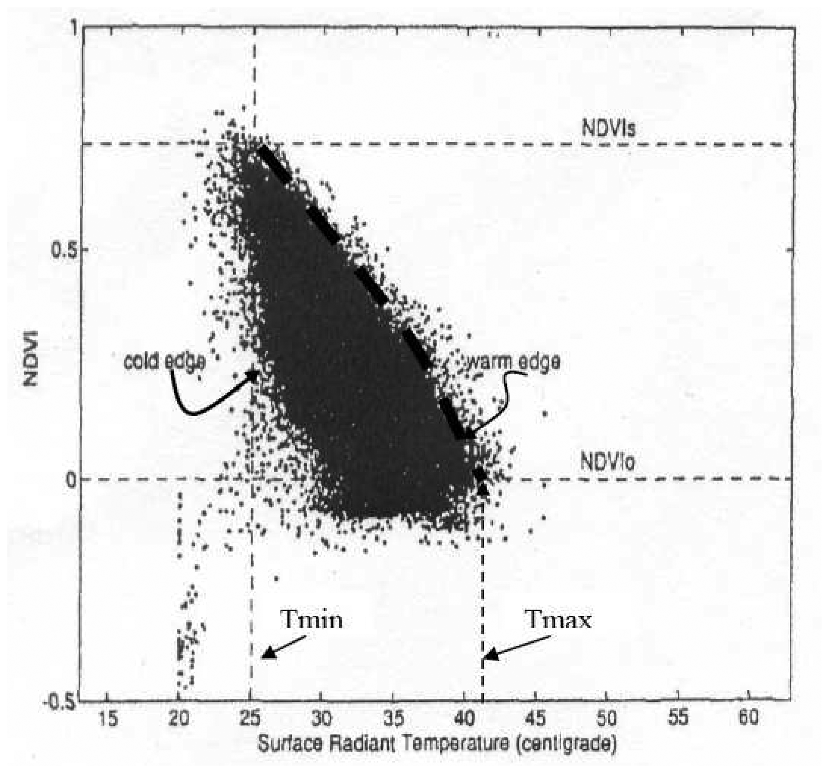
Several salient aspects of the triangle need to be explained. The scatter plots shown in Figures 1 and 2 slope toward the left (lower temperatures) with increasing vegetation fraction, a consequence of the fact that sunlit vegetation is generally cooler than sunlit bare soil. That the triangle exhibits a very small variation in Tir at dense vegetation (the top vertex of the triangle) is a crucial observation essential to modeling the pixel distribution (see section 2b). The warm and cold edges, labeled accordingly on Figure 2, thus refer to the soil surface radiant temperature limits in the image for the highest and lowest temperatures at a given fractional vegetation cover (or NDVI); as we will postulate, the vegetation temperature does not vary in space, so variations in temperature in the triangle reflect only the soil surface and therefore the soil surface dryness. Cold and warm edges, respectively, correspond to the wettest and driest pixels. A central assumption here is that, given a large number of pixels reflecting a full range of soil surface wetness and fractional vegetation cover, sharp boundaries in the data reflect real physical limits: i.e., bare soil, 100 percent vegetation cover, and lower and upper limits of the surface soil water content, e.g., completely dry or field capacity, respectively. The warm edge, denoted by the slanting heavy dashed line in Figure 2, thus corresponds to a dry soil surface soil limit, whereas the cold edge denotes a fully wetted soil surface.
As stated, highest and lowest values of NDVI, denoted respectively in Figure 1 as NDVIs and NDVIo, pertain to 100% vegetation cover and bare soil, respectively. The latter is analogous to the ‘line of soils’ in other types of representations (Price, 1990). As shown by Carlson and Ripley (1997), vegetation amounts can increase beyond the threshold at which Fr just reaches 100%, but with very little further increase of NDVI.
Outlying points, which here constitute a very small percentage of the whole, may represent anomalous surfaces, including standing water and cloud. It is quite likely in Figures 1 and 2 that the scatter of points below and to the left of the main envelope of points correspond to either cloud or standing water. In any case such points are discarded from analysis, or assigned default values for totally dry or wetted soil surfaces where pixels are close to the dry or wet edges.
In subsequent representations of the triangle, we will present the abscissa as a scaled surface radiant temperature T*, which varies from 0 (Tmin, the temperature pertaining to a dense clump of vegetation in well-watered soil) to 1.0 (Tmax, the temperature of dry, bare soil – represented by the highest temperatures in the image). Thus, we define T* as
where Tir is the surface radiant temperature, as shown in Figure 2, Similar formulations to that of T* have been made: using the surface air temperature instead of Tmin (Jiang and Islam, 1999) or the rate of rise of morning surface radiant temperature (Sandholt et al., 2002; Stisen et al., 2007). We will also transform the ordinate to fractional vegetation cover, using the algorithm
Some authors (Gutman and Ignatov, 1998) favor a linear relationship between NDVI and Fr, rather than the square shown in Equation 2. The advantage of this scaled version of the triangle is that both coordinate axes vary from 0 to 1.0 regardless of the amount of net radiation or the ambient air temperature. Here, both measured and model coordinates vary from 0 for well-watered vegetation (Tmin) to 1.0 for dry, bare soil (Tmax), respectively the left and right vertical dashed lines in Figure 2. Many authors tend to favor plotting un-scaled Tir versus NDVI, as in Figures 1 and 2, rather than scaling the data, although we favor scaling the coordinates because that yields a ‘universal’ triangle whose coordinates do not depend on ambient conditions. Scaling also reduces the sensitivity of Fr (and probably T*) to atmospheric correction (Carlson and Ripley, 1997), helps to isolate cloud and water pixels which tend to lie outside the triangle, and allows comparison of pixel data from different days and seasons within the same framework.
b) Modeling the triangle
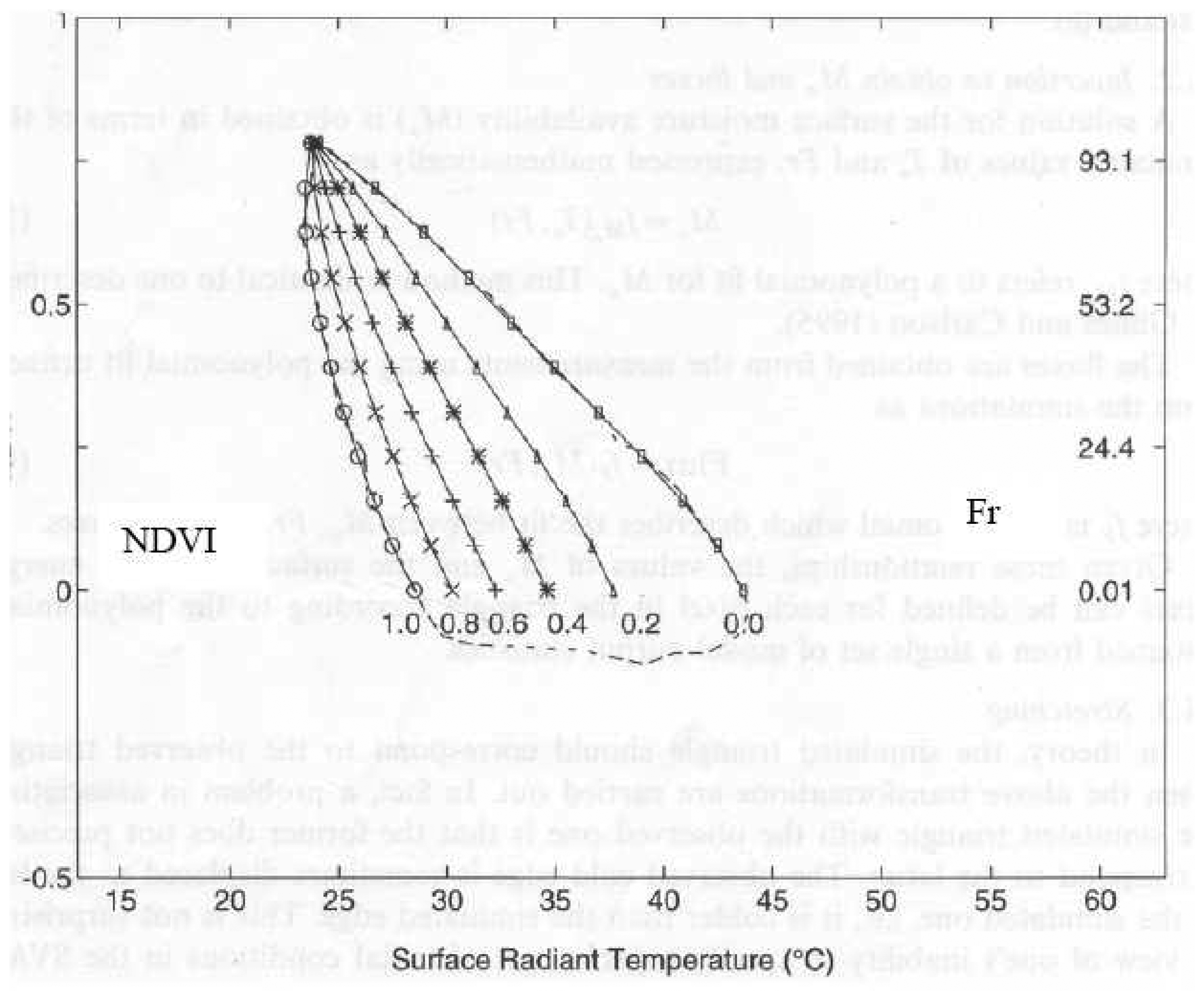
Primary input into the SVAT model referred to in this paper and used to create Figure 3 are a range of surface soil water content and fractional vegetation cover. Root zone soil water content, which governs the plant transpiration, is set at a value close to field capacity, thereby yielding an effective potential transpiration from the plants. Output consists of surface evapotranspiration, surface sensible heat flux, surface radiant temperature and other variables as a function of time during a 24 hour day; values pertaining to the time of satellite or aircraft overpass are used to compose the triangle. Given a complete range of surface soil water and Fr values as input and the assumption of potential transpiration for the leaves, this or any comparable SVAT model (such as the SEBAL model (Bastiaanssen et al., 2004)) would yield a triangular pattern of soil water content in Tir/Fr space, similar to the one used to compose Figure 3. Soil water content in our model is equated with a soil surface moisture availability, Mo, defined alternately as the ratio of soil surface evaporation (LEs) to the potential evaporation at the soil surface radiant temperature in patches of bare soil Ts (as opposed to Tir, the surface radiant temperature for the complete soil/vegetation canopy) or, alternately, as the ratio of soil water content to that at field capacity. (It should be noted that the definition of potential evaporation is not the same as that using the Penman or Priestly-Taylor equations.) Mo can also be expressed as the ratio of soil surface resistance to the soil surface plus atmospheric resistance. The equivalence of Mo to the fraction of field capacity has never been tested, but it seems a reasonable approximation, since both parameters vary from zero for completely dry soil to 1.0 for a fully wetted soil.
The SVAT model used to create Figure 3 is a 1-dimensional model developed at Penn State and called Simsphere (currently residing with ample documentation for user operation at http://www.agry.purdue.edu/climate/dev/Simsphere.asp). The figure shows the model solution expressed in T*/Fr space as isopleths of Mo, the soil surface moisture availability, and the evapotranspiration fraction EF, the latter defined as the ratio LE/Rn, where LE is the surface evapotranspiration (soil plus vegetation) and Rn is the net radiation at the surface. The solution, however, is intractable unless one crucial assumption is made which is based on the shape of the observed triangle: that the transpiration for the vegetation itself occurs at a constant (i.e., potential) value for all values of Mo and Fr. This condition requires that Mo becomes increasingly indeterminate and begin to merge as Fr approaches 1.0 at the vertex of the triangle. Although the pixel distribution sometimes appears truncated at the top of the triangle, model simulations show that a flattened top can be reproduced by allowing the thermal inertia in the model (a product of soil thermal conductivity and diffusivity) to increase with increasing soil water content. The other vertices, left and right, respectively, correspond to the condition for a totally wet soil (Mo=1.0; Fr=0; EF= LEs/Rn) and a completely dry soil (Mo=0; Fr=0; EF=0).
This assumption – that the transpiration occurs at near potential regardless of the surface soil water content – precludes any analysis of the water stress on vegetation using the triangle method. It merely formalizes the observation that Tir has little spatial variation at full vegetation cover, at least within the margin of measurement error. Although individual leaves subjected to water stress do tend to experience an increase in their radiant temperature, it is our observation that regardless of the soil water content (short of wilting) an ensemble of leaves comprising a dense vegetation cover tends to show little spatial variation in Tir.
It is important to note that while the Mo contours are almost straight lines, the EF isopleths are highly curved. Moreover, these isopleths show in EF decreasing with increasing Fr at high values of Mo, reflecting the fact that the stomatal resistance of vegetation impedes transpiration even when the soil is wet. When the soil is dry, however, soil surface evaporation becomes a less important component than for wet soil and therefore EF increases as a function of Fr along the warm edger. Islam (e.g., Jiang et al, 2004) use a factor β times Fr multiplied by the potential transpiration at a given Fr to account for the reduction of transpiration below potential. This mathematical device, however, does not capture the previously mentioned reversal in the change in EF with decreasing Fr between wet and dry soils.
Given both model and image values of T*, derived from their respective Tmax and Tmin, the model triangle is effectively stretched over the observed one, thereby defining all measured pixel values within the triangle in terms of the model output. A virtue of the triangle method is that regardless of the net radiation or changes in ambient temperature from one day to the next (such as might occur after the passage of a cold front) or differences of the satellite or aircraft measurement time, a similar triangle is generated over a succession of days with a more or less identical configuration of EF and Mo isopleths within the triangle.
Islam and others (e.g., Jiang and Islam, 1999) adopt slightly different approaches. They also specify potential transpiration from vegetation, using, for example, the Priestly-Taylor relationship or a Penman-Monteith one, but with an adjustment to account for the effects of stomatal resistance. The temperature variable is expressed as a difference (ΔT =Tir-Tw), where Tw, similar to Tmin, is some reference cool temperature, either that of a water surface or an air temperature or that over a completely wetted surface. Air temperature also provides an estimate for Tw, which can be obtained directly from the triangular pixel distribution by assuming that the temperature at the vertex of the triangle corresponds to that equal to or slightly above air temperature (Prihodko et al.., 1997). For example, a good choice of air temperature in Figure 2 would be Tmin, or that corresponding to the left-hand vertical dashed line at To=25 C (or perhaps something slightly lower). Thus, the ΔT used by Islam and his associates is essentially T*. Stisen et al. (2007) use the rate of rise of morning temperature, as defined from a succession of satellite images, as the variable ΔT. The latter is also very similar to T*.
Figure 4 shows the modeled moisture availability isopleths superimposed on the pixel distribution in Figure 2, Mo = 0 and 1.0, respectively, corresponding to the warm and cold edges. Stretching implies that the derived values for Mo and EF are relatively insensitive to the choice of initial conditions, as the isopleths within the triangle will not change their configuration drastically with any reasonable choice of those conditions. Thus, Mo=0 and Mo=1 will always border the pixel envelope and Mo=0.5 will always appear somewhere in the middle of the triangle. The same is true for the relative stability of EF isopleths within the triangle.
3. Practical applications
In principle, the triangle method works with any reasonable land surface model. The model serves merely to create the relationship between measured Tir and Fr and the EF and Mo values. Our approach is to use the model once to create a matrix of T* and EF values for an entire range of input Fr and Mo values, given a fixed set of ancillary input variables such as surface albedo and stomatal resistance. From this matrix, a set of polynomials are generated, which are then used to calculate Mo and EF for all pixel values.
The relationships for Mo and EF are given by third order polynomial with cross products as
where the subscripts i and j pertain to the modeled surface radiant temperature T* (defined in Equation 1) and the fractional vegetation cover; the coefficients for the two surface parameters are given in Tables 1a and 1b. The multiple correlation coefficient, R-square, for both parameters are very close to 1.0 and the RMSE (root mean squared error) between the polynomial values and raw model output is less than 2 percent.
A reasonable fit for the warm edge is also given by a polynomial fit to the simulated model output.
where the coefficients for the polynomial are given in Table 2. T*edge in Equation 4 determines the value of T* along the warm edge, which can assume values less than or equal to 1.0 depending on the value of Fr.
Admittedly, these relationships would not precisely fit every situation, but the fields of EF and Mo expressed by Tables 1 and 2 are probably sufficiently accurate (and certainly very convenient to use) for many applications where a suitable SVAT model is not available. These polynomials require relatively little expense in computer time or human resources in processing large images. It is important to note that specifying the form of the cold edge is not necessary here, as Tmin is the essential variable for the cold side of the pixel envelope (ref. Equation 1) and for calculating T*.
4. Qualitative Interpretation of the Triangle
Transforming the pixel values to those of Mo and EF using the polynomial, in effect, stretches the model triangle over the measured one. As previously stated, this transformation of the Tir/Fr space establishes the triangle (more precisely the relative configuration of its internal isopleths) as close to being invariant over a succession of images, regardless of the change in atmospheric conditions. One image can provide only a snapshot of the soil surface moisture. It is possible, however, to speak of a ‘universal’ triangle, which has a further dimension: that of time. Not only do a succession of images show the changing surface wetness and evapotranspiration in the face of periods of precipitation and surface drying, but pixel values representing the same surface element, as determined from a succession of images, describe trajectories in time within a single triangle. The patterns produced by such trajectories provide a unique signature for the land use transformation (Lambin and Erhlich, 1996). Moreover, it is not uncommon to find swarms of similar trajectories constituting a swath of pixels whose orientation suggests the evolution of land use. In a particular area.
For example, Figure 5 shows the location of individual pixels within a triangle composed for an image over part of Costa Rica, including its capital, San Jose' (Carlson and Sanchez-Azofeifa, 1999). Pixels classed as urban (U), forest (F), pasture (P) or crop (S) are labeled. Not surprisingly, urban pixels cluster near the lower part of the triangle, while pasture and forest cluster near the top. Overall, the distribution of pixels suggests two or possibly three distinct swaths, oriented from the upper left side to the lower right side of the triangle. These swaths also tend to cross from higher to lower values of Mo and EF, almost at right angles to the latter.
For example, Gillies and Carlson (1995) showed how seasonal changes in the surface fabric are captured by the pixel trajectories, which form closed loops. Irreversible land use changes, however, prescribe more open paths which do not return to their ‘origins’. The latter is illustrated in Figure 6. We found that the swaths correspond to three small clusters of pixels, largely found along the outer part of the urban area constituting the city of San Jose; these will be designated by the letters A, B and C. We followed those pixels for seven years, starting with 1990 and ending in 1997; these are denoted by two continuous arrow segments in Figure 6, one for 1990-1995 and the other for 1995-1997. Trajectory cluster A moves from the western edge of San Jose', which is mostly suburban development with a moderate urban growth rate with some vegetation cover and a dry surface, toward lower vegetation and lower EF without much change in surface wetness (Mo). Trajectory B, representing points in the south and central part of the city, changes Mo and EF values more rapidly than trajectory A. Trajectory C is similar to that of A except that the development from agricultural to urban land use was much further advanced. In all three cases urbanization takes the pixels toward the lower right hand corner of the triangle. These trajectories represent huge changes in urbanization in just seven years.
Similar analyses pertaining to land use changes around a lake in Pennsylvania were shown by Carlson and Arthur (2000). As in the Costa Rica study, trajectories tend to move toward lower values of Mo and EF, though often with only a gradual crossing of Mo isopleths.
In these types of analyses, each land use transformation has its own characteristic signal. A somewhat surprising aspect in Figure 6 is that points moving toward lower Fr change Mo very gradually, though they cross more sharply to lower values of EF. Trajectory A in Figure 6 almost maintains a constant (albeit low) value of Mo, though EF is changing rapidly with time because more and more of the dry bare surface is being exposed. Ultimately, of course, complete urbanization requires that the trajectories reach the lower right vertex of the triangle.
The significance of the swaths is that their orientation suggests a favored path for points undergoing similar land use changes as they undergo urbanization and progress toward lower values of EF and Mo. The assumption that the slope of the swath prescribes a surface canopy resistance, as claimed by Nemani and Running (1989), is not quite correct because the swaths do not imply a uniform surface fabric. It is true, however, that a swath having the same slope as the Mo isopleth will correspond to pixels having approximately the same soil surface resistance, because, according to the definition of moisture availability (air resistance divided by air plus surface resistance), Mo is largely controlled by the surface resistance and its lack of change in Mo following a trajectory toward lower Fr is largely due to the reduction of vegetation amount rather than a decrease in the exposed soil surface wetness.
5. Limitations of the Triangle Method Time
The most severe limitation of the triangle method is that identification of the triangular shape in the pixel distribution requires a flat surface and a large number of pixels over an area with a wide range of soil wetness and fractional vegetation cover. Although not of first order importance, determination of the warm edge and the vegetation limits of bare soil and full cover requires some subjectivity. Nevertheless, the triangle method is effective with higher resolution imagery, such as those from Landsat or aircraft radiometers, because the triangle is more easily resolved than for AVHRR imagery. Nevertheless, Figure 1, though obtained from an AVHRR image, contains sufficient points to define a triangle because of the large number of data points, although the definition of the triangle requires more subjectivity than with higher resolution imagery.
Another difficulty is the use of a SVAT model, which requires some familiarity with the physics and in its initialization and operation on the part of the user, especially for regions where knowledge of the soil and vegetation characteristics is sketchy.
In practice, however, it is not necessary to specify many input parameters for the SVAT model with great accuracy. Nor is there need for the image to contain a complete spectrum of surface radiant temperatures and vegetation cover, as long as some patches of bare, dry ground and of dense vegetation can be resolved with sufficient number of pixels with to engender confidence in a representative value for each type of surface. Thus, it is often possible to locate a city center having enough pixels to assign a value of Tmax, while a stand of trees might adequately represent dense vegetation and a value of Tmin. These temperature extremes sometimes can be determined with some confidence even for AVHRR imagery even where the number of pixels in the image is not very large, as shown in Figure 7. Here, the warm edge is distinct, though the bare soil extreme is somewhat uncertain, having been set, probably incorrectly in this example (Owen et al., 1998), at zero; a value of 0.3 (dotted line) now seems a better choice. In a study by Carlson et al. (1995), in which high resolution (aircraft; NS001) imagery was successively degraded from that of 5 m, it was shown that the warm edge remains distinct to a resolution of 80 and possibly to at least 320 m.
Finally, it is necessary to emphasize a limiting aspect of all remotely based measurement systems based on the interpretation of the thermal infrared signal: the latter is capable of sensing the soil moisture only over the top centimeter or two of the bare soil surface visible to the radiometer field of view. On the other hand, the values of ET and surface sensible heat flux are directly related to the surface soil water content and are, therefore, highly appropriate quantities to measure using thermal infrared sensors.
6. Summary
The triangle method has the capability of producing non-linear solutions for surface moisture availability and surface evapotranspiration from large image data sets. These important variables can be generated quickly with relative ease, since a solution need be established only once for a series of images. The triangle method also has the virtue of requiring no ancillary atmospheric or surface data or any special land surface model and it is relatively insensitive to atmospheric correction or the choice of ambient atmospheric and surface parameters in whatever land surface model is used. This is because the pixel distribution itself is used to set a set of conditions required to produce a solution for surface soil wetness and evapotranspiration fraction. By creating a ‘universal’ triangle, in which the model triangle is effectively stretched over the measured one, the triangle can accommodate a succession of images, thus adding the dimension of time. Plotting the trajectories of pixel points from a succession of images within the triangle as a function of time illuminates the nature of land use change, either from seasonal variations or as the result of urbanization.
In general the triangle method is able to achieve an accuracy comparable to other methods in that the errors in estimating EF are typically ±0.1- 0.2. As shown by Jiang et al., (2004), such errors may be close to the minimum practically achievable by remote sensing.
The main weakness of the triangle method is that it requires some subjectivity in identifying the warm edge and the dense vegetation and bare soil extremes. Identification is more easily obtained from high resolution imagery or at least images with a sufficient numbers of pixels such that they define a range in land surface wetness and vegetation cover or, at least, the vegetation and wetness extremes.
References
- Bastiaanssen, W.G.M.; Menenti, M.; Feddes, R.A.; Holtslag, A.A.M. A Remote Sensing Surface Energy Balance Algorithm for Land (SEBAL) - 2.Validation. Journal of Hydrology 1998, 213, 198–212. [Google Scholar]
- Bastiaanssen, W.G.M.; Noordman, E.J.M.; Pelgrum, H.; Davids, G.; Allen, R.G. SEBAL for spatially distributed ET under actual management and growing conditions. ASCE Journal of Irrigation and Drainage Engineering 2005, 131, 85–93. [Google Scholar]
- Carlson, T.N.; Dodd, J.K.; Benjamin, S.G.; Cooper, J.N. Remote Estimation of Surface Energy Balance, Moisture Availability and Thermal Inertia. J. Appl. Meteor. 1981, 20, 67–87. [Google Scholar]
- Carlson, T.N.; Rose, F.G.; Perry, E.M. Regional Scale Estimates of Surface Moisture Availability from GOES Satellite. Agron. J. 1984, 76, 972–979. [Google Scholar]
- Carlson, T.N.; Gillies, R.R.; Perry, E.M. A Method to Make Use of Thermal Infrared Temperature and NDVI measurements to Infer Surface Soil Water Content and Fractional Vegetation Cover. Remote Sensing Reviews 1994, 9, 161–173. [Google Scholar]
- Carlson, T.N.; Gillies, R.R.; Schmugge, T.J. An Interpretation of Methodologies for Indirect Measurement of Soil-Water Content. Agricultural and Forest Meteorology 1995, 77, 191–205. [Google Scholar]
- Carlson, T.N.; Ripley, D.A.J. On the Relationship Between NDVI, Fractional Vegetation Cover and Leaf Area Index. Remote Sensing Environment 1997, 62, 241–252. [Google Scholar]
- Carlson, T.N.; Sanchez-Azofeifa, G.A. Satellite remote sensing of land use changes in and around San Jose, Costa Rica. Remote Sensing of Environment 1999, 70, 247–256. [Google Scholar]
- Carlson, T.N.; Arthur, A.T. The Impact of Land Use – Land Cover Changes Due to Urbanization on Surface Microclimate and Hydrology: A Satellite Perspective. Global and Planetary Change 2000, 25, 49–65. [Google Scholar]
- Chauhan, N.; Miller, S.S.; Ardanuy, P. Spaceborne soil moisture estimation at high resolution: a microwave-optical/IR synergistic approach. International Journal of Remote Sensing 2003, 22, 4599–4622. [Google Scholar]
- Crombie, M.K.; Gillies, R.R.; Avidson, R.E.; Brookmeyer, P.; Weil, G.J.; Sultan, M.; Harb, M. An Application of Remotely Derived Climatological Fields for Risk Assessment of Vector-borne Diseases – A Spatial Study of Filariasis Prevalence in the Nile Delta, Egypt. Photogramm. Eng. Remote Sensing 1999, 65, 1401–1409. [Google Scholar]
- Gillies, R.R.; Carlson, T.N. Thermal Remote Sensing of Surface Soil Water Content with Partial Vegetation Cover for Incorporation into Climate Models. Journal of Applied Meteorology 1995, 34, 745–756. [Google Scholar]
- Gillies, R.R.; Carlson, T.N.; Cui, J.; Kustas, W.P.; Humes, K.S. A verification of the ‘triangle’ method for obtaining surface soil water content and energy fluxes from remote measurements of the Normalized Difference Vegetation Index (NDVI) and surface radiant temperature. International Journal of Remote Sensing 1997, 18, 3145–3166. [Google Scholar]
- Gillies, R.R.; Temesgen, B. Coupling Thermal Infrared and Visible Satellite Measurements to Infer Biophysical Variables at the Land Surface. In Thermal Remote Sensing in Land Surface Processes; Quattrochi, Luval, Eds.; CRC Press, 2004. [Google Scholar]
- Gutman, G.; Ignatov, A. The Derivation of the Green Vegetation Fraction from NOAA/AVHRR Data for Use in Numerical Weather Prediction Models. Int. J. of Remote Sensing 1998, 8, 1533–1543. [Google Scholar]
- Jiang, L.; Islam, S. A Methodology for Estimation of Surface Evapotranspiration over Large Areas using Remote Sensing Observations. Geophysical Research Letters 1999, 26, 2773–2776. [Google Scholar]
- Jiang, L.; Islam, S. Estimation of Surface Evaporation Map over Southern Great Plains Using Remote Sensing Data. Water Resources Research 2001, 37, 329–340. [Google Scholar]
- Jiang, L.; Islam, S. An Intercomparison of Regional Latent Heat Flux Estimation using Remote Sensing Data. International Journal of Remote Sensing 2003, 24, 2221–2236. [Google Scholar]
- Jiang, L.; Islam, S.; Carlson, T.N. Uncertainties in latent heat flux measurement and estimation: implications for using a simplified approach with remote sensing data. Canadian Journal of Remote Sensing 2004, 30, 769–787. [Google Scholar]
- Kustas, W.P. Estimates of Evapotranspiration with a One- and Two-layer Model of Heat Transfer Over Partial Canopy Cover. J. Appl., Meteor. 1990, 29, 205–223. [Google Scholar]
- Kustas, W.P.; Norman, J.M. Use of Remote Sensing for Evapotranspiration Monitoring Over Land Surfaces. Hydrological Sciences Journal 1996, 41, 495–516. [Google Scholar]
- Lambin, E.G.; Ehrlich, D. The Surface Temperature-vegetation Index Space for Land Cover and Land-cover Change Analysis. Int. J. Remote Sensing 1996, 17, 463–487. [Google Scholar]
- Liang, S. Quantitative Remote Sensing of Land Surfaces.; Wiley Series on Remote Sensing; 2004; p. 536 pp. [Google Scholar]
- Margulis, S.A.; Kim, J.; Hogue, T. A Comparison of the Triangle Retrieval and Variational Data Assimilation Methods for Surface Turbulent Flux Estimation. J. Hydromet. 2005, 6, 1063–1072. [Google Scholar]
- Mecikalski, J.R.; Diak, G.R.; Anderson, M.C.; Norman, J.M. Estimating Fluxes on Continental Scales using Remotely Sensed Data in an Atmospheric-land Exchange Model. J. Appl. Meteor. 1999, 38, 1352–1369. [Google Scholar]
- Moran, M.S.; Clarke, T.R.; Kustas, W.P.; Weltz, M.; Amer, S.A. Evaluation of Hydrologic Parameters in A Semiarid Rangeland Using Remotely-Sensed Spectral Data. Water Resources Research 1994, 30, 1287–1297. [Google Scholar]
- Nemani, R.R.; Running, S.W. Estimation of Regional Surface-Resistance to Evapotranspiration from NDVI and Thermal-IR AVHRR Data. Journal of Applied Meteorology 1989, 28, 276–284. [Google Scholar]
- Owen, T.W.; Carlson, T.N.; Gillies, R.R. An Assessment of satellite Remotely-sensed Land Cover Parameters in Quantitatively Describing the Climatic Effect of Urbanization. Int. J. Remote Sensing 1998, 19, 1663–1681. [Google Scholar]
- Petropoulis, G.P.; Wooster, M.J.; Drake, N.J. Investigating the Performance of a Coupled SVAT/Model Remote Sensing Method to Derive Spatially Explicit Maps of Land Atmosphere Energy Fluxes; Geophysical Research Abstracts, 0634, European Geosciences Union, 2006; ISBN: SRef ID: 1607-7962. [Google Scholar]
- Price, J.C. The Potential of Remotely Sensed Thermal Infrared Data to Infer Surface Soil Moisture and Evaporation. Water Resources Research 1980, 16, 787–795. [Google Scholar]
- Price, J.C. Estimation of Regional Scale Evapotranspiration through Analysis of Satellite thermal-infrared Data. IEEE Transactions on Geoscience and Remote Sensing 1982, GE-20, 286–292. [Google Scholar]
- Price, J.C. Using Spatial Context in Satellite Data to Infer Regional Scale Evapotranspiration. IEEE Transactions on Geoscience and Remote Sensing 1990, 28, 940–948. [Google Scholar]
- Prihodko, L.; Goward, S.N. Estimation of air temperature from remotely sensed surface observations. Remote Sensing of Environment 1997, 60, 335–346. [Google Scholar]
- Ray, D.K.; Nair, U.S.; Welch, R.M.; Su, W.; Kikutchi, T. Influence of land use on the regional climate of southwest Australia. 13th Symposium on Global Change and Climate Variations and 16th Conference on Hydrology, Australia, Jan, 17, 2002; 2002. Available on http://ams.confex.com/ams/annual2002/techprogram/paper_29880.htm.
- Sandholt, I.; Rasmussen, K.; Andersen, J. A simple interpretation of the surface temperature/vegetation index space for assessment of surface moisture status. Remote Sensing of Environment 2002, 79, 213–224. [Google Scholar]
- Stisen, S.; Sandholt, I.; Norgaard, A.; Fensholt, R.; Jensen, K.H. Combining the Triangle Methodl with Thermal Inertia to Estimate Regional Evapotanspiration – Applied to MSG-SEVIRI Data in the Senegal River Basin. Remote Sensing Environment 2007, in press. [Google Scholar]
- Seguin, B.; Itier, B. Using Midday Surface-Temperature to Estimate Daily Evaporation from Satellite Thermal Ir Data. International Journal of Remote Sensing 1983, 4, 371–383. [Google Scholar]
- Soer, G.J.R. Estimation of Regional Evapotranspiration and Soil Moisture Conditions using Remotely Sensed Crop Surface Temperatures. Remote Sensing Environment 1980, 9, 27–45. [Google Scholar]
- Stewart., J.B.; Kustas, W.P.; Humes, K.S.; Nichols, W.D.; Moran, M.S.; De Bruin, H.A.R. Sensible Heat Flux-Radiant Surface Temperature Relationship for Semiarid Areas. J. Appl. Meteor. 1994, 33, 1110–1117. [Google Scholar]
- Watson, K. Applications of Thermal Modeling in the Geological Interpretation of IR Images. Proceedings of the Seventh Int. Symposium of Remote Sensing of Environment. ERIM., Ann Arbor, MI. 1971; pp. 2017–2041. [Google Scholar]
- Wetzel, P.; Atlas, D.; Woodward, R. Determining Soil Moisture from Study. J. Climate and Applied Meteor. 1983, 23, 375–391. [Google Scholar]
Figure 1.
Scatter plot of satellite pixel values of NDVI versus radiant surface temperature from an AVHRR image approximately 100 km on a side located near Philadelphia, Pennsylvania, August 17, 1991. The warm edge, denoted with an arrow, is evident from the sharply defined right side of the pixel envelope. Pixels likely representing clouds and water are labeled with arrows.

Figure 2.
Scatter plot of NDVI versus surface radiant temperature for an NS001 image over Walnut Gulch, Arizona during summertime. Salient features of the triangle are: the maximum and minimum temperatures as vertical, dashed lines (Tmax and Tmin), the warm edge (heavy dashed line), the cold edge and the limits for dense vegetation (NDVIs) and bare soil (NDVIo).

Figure 3.
Model simulated triangle showing fractional vegetation cover (Fr; %) versus scaled radiant surface temperature (T*) (see definition in text). Slanting, nearly straight, lines represent the soil surface soil moisture availability, Mo labeled at intervals of 0.1, increasing from 0 on the right side (the warm edge). Curved lines labeled as fractions represent the evapotranspiration fraction, EF.

Figure 4.
Isopleths of moisture availability (Mo) overlaying the pixel envelope shown in Figure 2, as determined from the SVAT model. The ordinate values are plotted as NDVI (left side) and fractional vegetation cover (Fr; right side) and the abscissa is the radiant temperature. The thin curvy line below the Mo labels denotes the bottom part of the pixel envelope in Figure 2.

Figure 5.
Scatterplot of selected pixels within the triangle, whose axes are labeled as Fr and T*, for an AVHRR image over a region around San Jose', Costa Rica, on 24 December, 1990. Pixels are labeled as either forest (F), pasture (P), urban (U) or cropland (S). The nearly straight lines slanting upward toward the left are isopleths of Mo at intervals of 0.1 (ranging from zero along the warm edge to 1.0 at the cold side of the distribution). The curved lines labeled in fractions (all except for the dashed line representing the 0.55 value) are isopleths of EF.

Figure 6.
Average trajectories of clusters A, B and C (roughly determined from the scatter plot in Figure 5) for the period 1990 – 1995 and 1995-1997 (the two arrow segments for each cluster).
Figure 6.
Average trajectories of clusters A, B and C (roughly determined from the scatter plot in Figure 5) for the period 1990 – 1995 and 1995-1997 (the two arrow segments for each cluster).

Figure 7.
Scatter plot of NDVI versus Tir for an AVHRR image over Central Pennsylvania, 14 June, 1994. Tmax and Tmin, as defined in the text are shown, along with the limits for bare soil NDVI (NDVIo) and that for dense vegetation NDVIs. The horizontal dotted line suggests a possibly better value of NDVIo, than that originally chosen in the article by Owen et al. (1998).


Table 1.
Coefficients of the polynomial relationship for Mo (a; top) and EF (b; bottom) between T* and Fr as specified in Equation 3.
| aij | j=0 | j=1 | j=2 | j=3 |
|---|---|---|---|---|
| i=0 | 2.058 | -1.644 | 0.850 | -0.313 |
| i=1 | -6.490 | 1.112 | -3.420 | -0.062 |
| i=2 | 7.618 | 3.494 | 10.869 | 4.831 |
| i=3 | -3.190 | -3.871 | -6.974 | -16.902 |
| aij | j=0 | j=1 | j=2 | j=3 |
| i=0 | 0.8106 | -0.5967 | 0.4049 | -0.0740 |
| i=1 | -0.8029 | 0.7537 | 0.0681 | 0.2302 |
| i=2 | 0.4866 | 1.2402 | -0.9489 | -0.8676 |
| i=3 | -0.3702 | -1.3943 | -0.7359 | 0.3860 |
Table 2.
Coefficients for the polynomial relating the temperature along the warm edge and Fr as specified in Equation 4.
| Edge | b | a1 | a2 | r2 | RMSE |
|---|---|---|---|---|---|
| (Warm Edge)Mo=0 | 1.001 | -0.892 | 0.075 | 1 | 0.0009 |
| (Cold Edge)Mo=1 | 0.216 | -0.366 | 0.149 | 1 | 0.0005 |
© 2007 by MDPI ( http://www.mdpi.org). Reproduction is permitted for noncommercial purposes.
Share and Cite
MDPI and ACS Style
Carlson, T. An Overview of the "Triangle Method" for Estimating Surface Evapotranspiration and Soil Moisture from Satellite Imagery. Sensors 2007, 7, 1612-1629. https://0-doi-org.brum.beds.ac.uk/10.3390/s7081612
AMA Style
Carlson T. An Overview of the "Triangle Method" for Estimating Surface Evapotranspiration and Soil Moisture from Satellite Imagery. Sensors. 2007; 7(8):1612-1629. https://0-doi-org.brum.beds.ac.uk/10.3390/s7081612
Chicago/Turabian StyleCarlson, Toby. 2007. "An Overview of the "Triangle Method" for Estimating Surface Evapotranspiration and Soil Moisture from Satellite Imagery" Sensors 7, no. 8: 1612-1629. https://0-doi-org.brum.beds.ac.uk/10.3390/s7081612