Geographically Weighted Regression Models in Estimating Median Home Prices in Towns of Massachusetts Based on an Urban Sustainability Framework

Abstract
:1. Introduction
1.1. Background
1.2. Modeling Framework
2. Materials and Methods
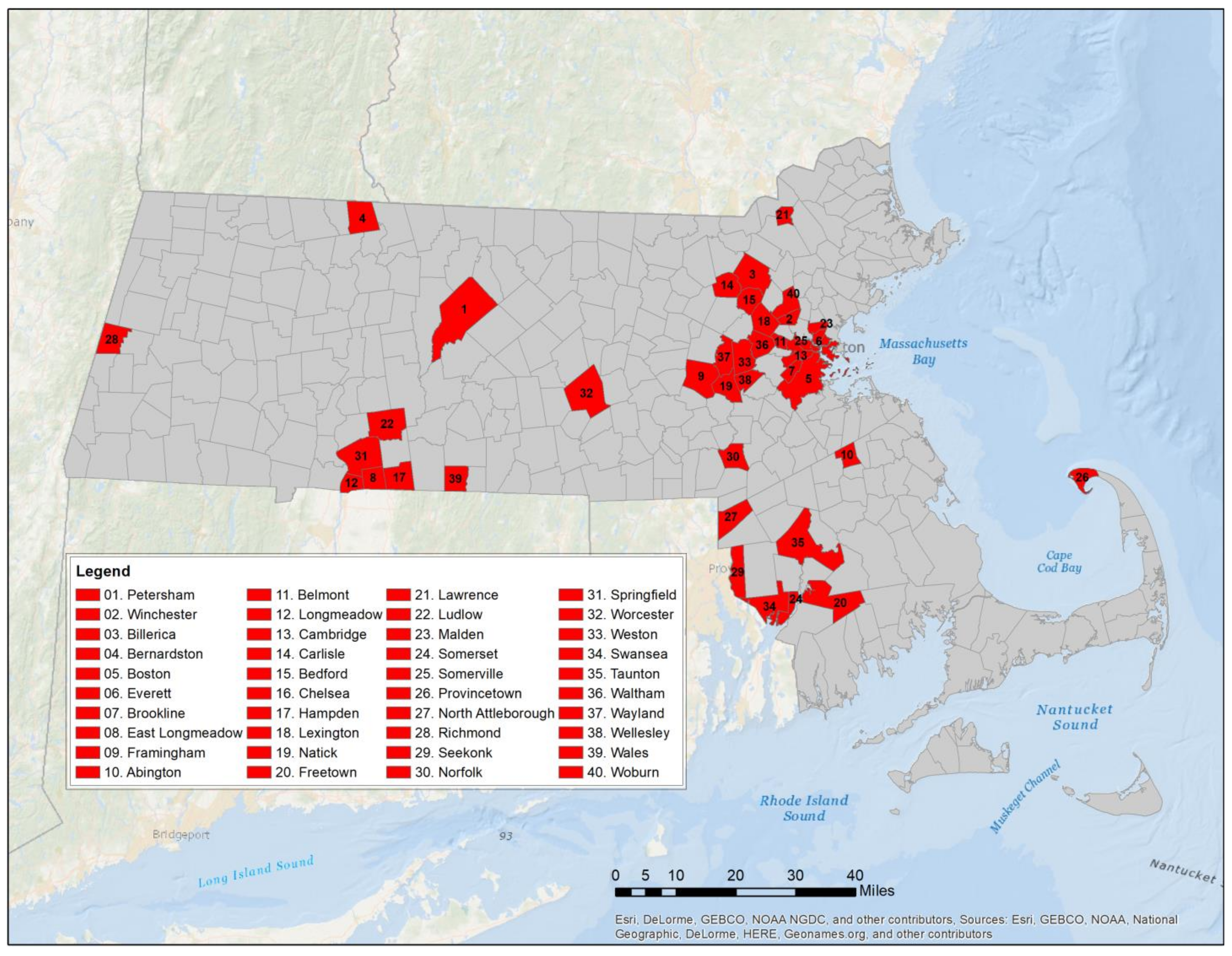
2.1. Study Area
2.2. Data Sources—Socio-Economic and Environmental Variables
2.3. Spatial Model Considerations
- is the dependent variable at location
- is the th independent variable at location
- is the number of independent variables
3. Results
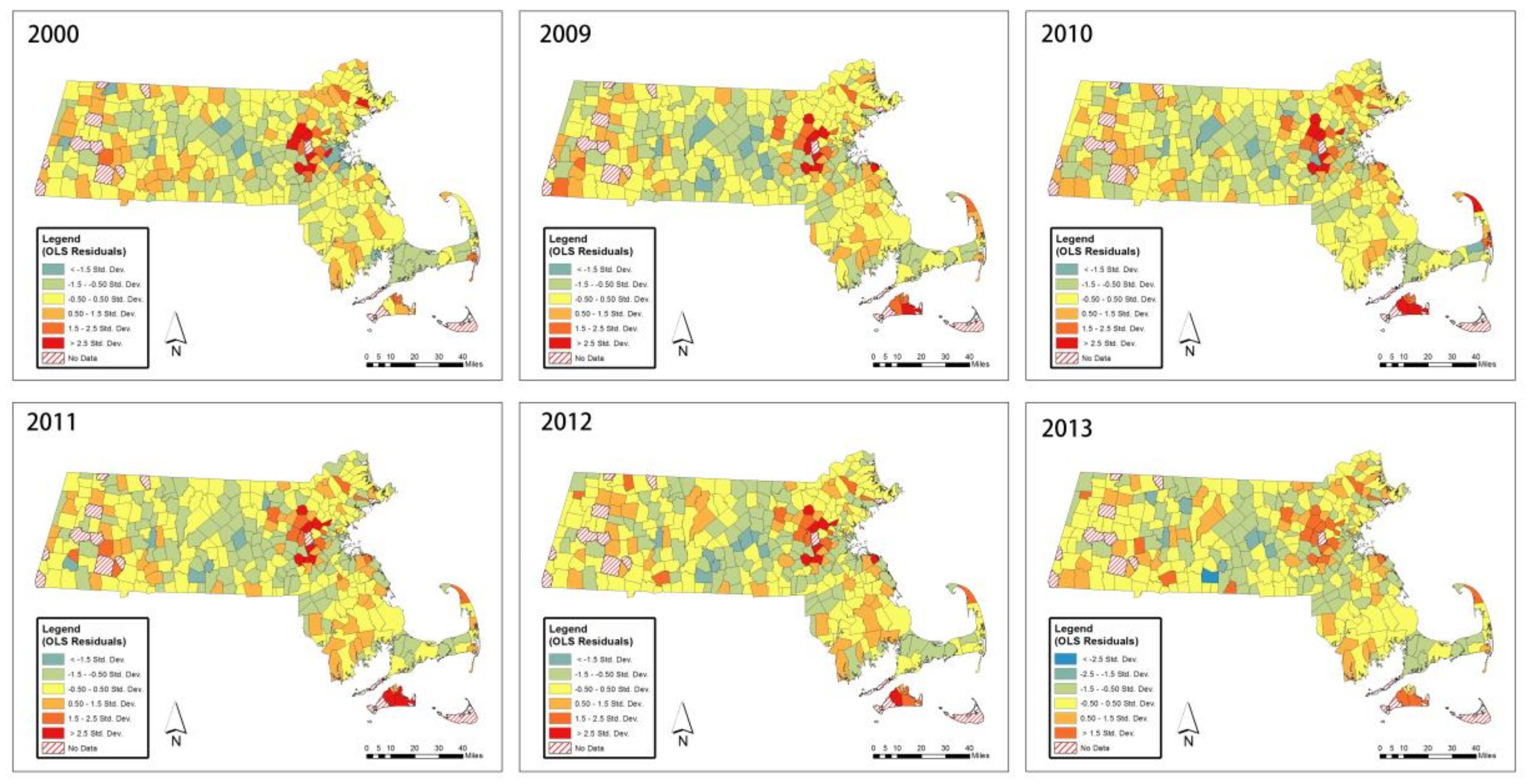
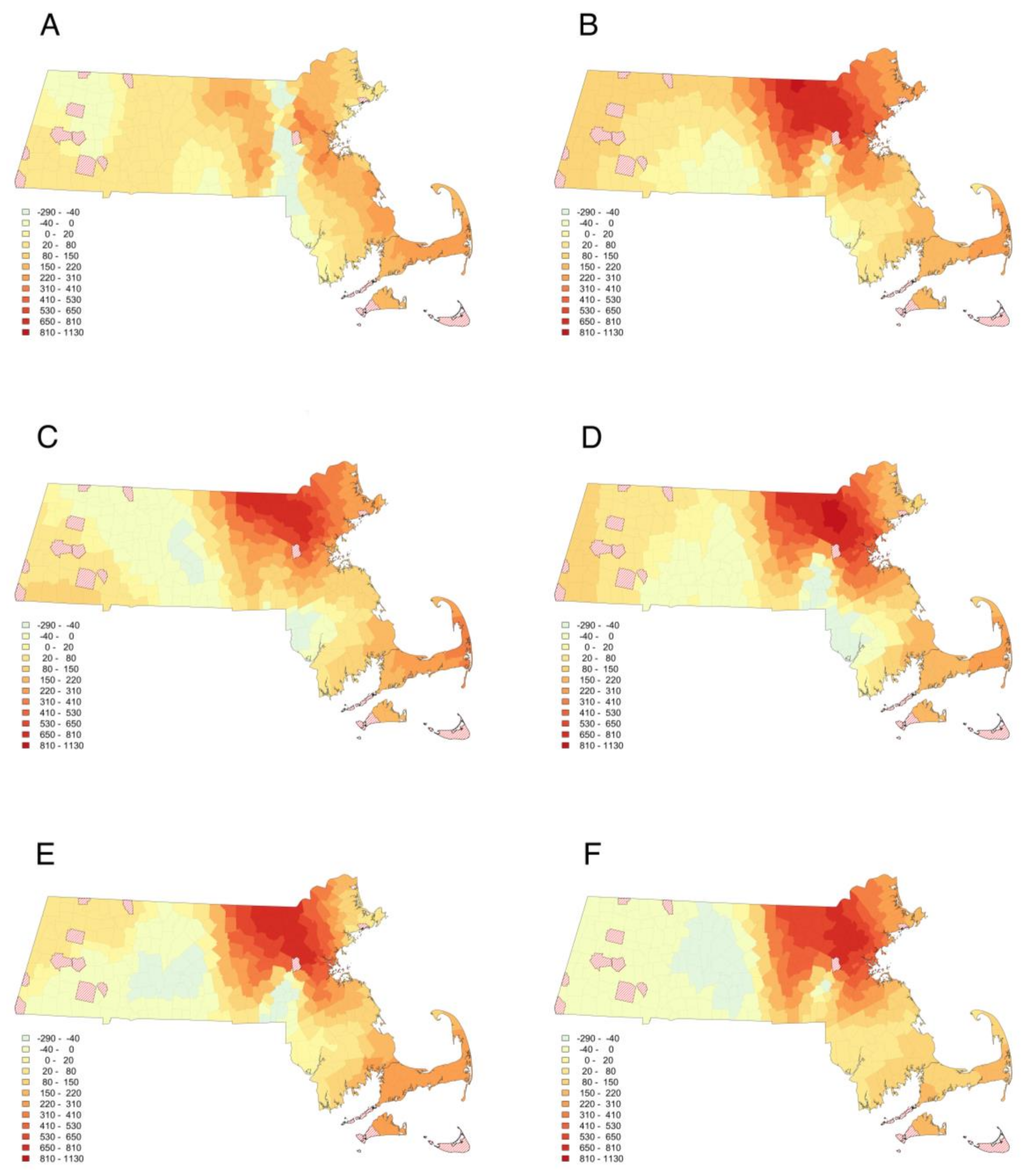
3.1. Spatial-Temporal Patterns of Home Prices
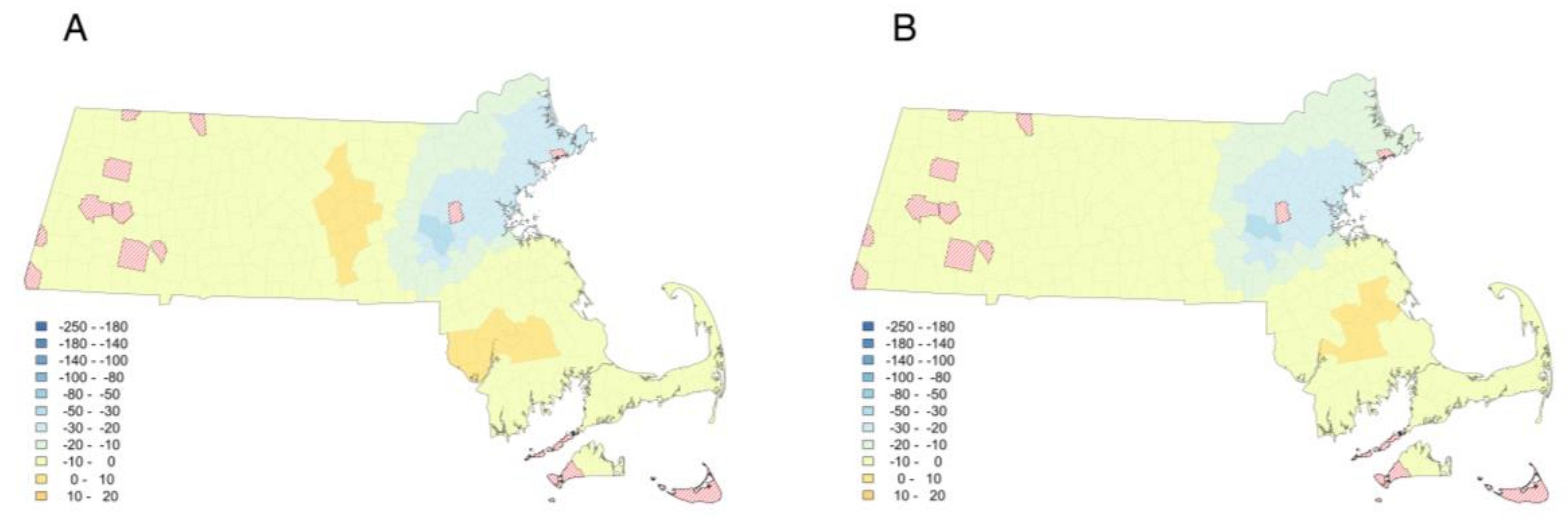
3.2. Are All Determinants of Median Home Price Non-Stationary?
3.3. Impact of Housing on Urban Sustainability
4. Discussion
5. Conclusions
Supplementary Materials
Acknowledgments
Author Contributions
Conflicts of Interest
Appendix A

| Median Home Price | |||||||
|---|---|---|---|---|---|---|---|
| Basic GWR Model (2000) | |||||||
| Variables | Minimum | Median | Max | % of Positive | % of Negative | p-Value (F3) | Sig. |
| Intercept | −212.70 | 243.24 | 1190.76 | 90.77 | 9.23 | 1.47 × 10⁻¹¹ | *** |
| Population Density | −11.92 | 0.68 | 28.78 | 60.71 | 39.29 | 0.5142965 | - |
| Unprotected Forest | −217.68 | 68.88 | 388.90 | 84.52 | 15.48 | 0.3060173 | - |
| Unemployment Rate | −189.08 | −17.66 | 16.92 | 11.31 | 88.69 | <2.2 × 10⁻¹⁶ | *** |
| Residential Area | −756.43 | −73.39 | 300.69 | 35.71 | 64.29 | 0.0004993 | *** |
| Vehicle ownership | −1323.53 | −162.52 | 229.86 | 9.82 | 90.18 | <2.2 × 10⁻¹⁶ | *** |
| Higher Education | 297.39 | 1110.62 | 1985.25 | 100 | 0 | 6.85 × 10⁻¹³ | *** |
| Senior Population | −522.05 | 226.41 | 1470.80 | 84.82 | 15.18 | 1.04 × 10⁻¹¹ | *** |
| Dist. to Stations | −8.48 | −0.18 | 16.72 | 39.88 | 60.12 | 3.59 × 10⁻⁶ | *** |
| Property Tax | −20.63 | −3.48 | 1.38 | 10.12 | 89.88 | 6.51 × 10⁻¹² | *** |
| CPI | −1.37 | 1.38 | 6.78 | 80.65 | 19.35 | 0.040276 | * |
| Median Home Price | |||||||
|---|---|---|---|---|---|---|---|
| Basic GWR Model (2010) | |||||||
| Variables | Minimum | Median | Max | % of Positive | % of Negative | p-Value (F3) | Sig. |
| Intercept | −130.54 | 347.02 | 1501.33 | 97.92 | 2.08 | 3.07 × 10⁻² | * |
| Population Density | −11.22 | 2.30 | 25.15 | 78.27 | 21.73 | 0.531882 | - |
| Unprotected Forest | −61.80 | 100.84 | 745.17 | 77.08 | 22.92 | 1.90 × 10⁻¹³ | *** |
| Unemployment Rate | −114.97 | −15.33 | 3.10 | 2.68 | 97.32 | <2.2 × 10⁻¹⁶ | *** |
| Residential Area | −781.96 | −107.39 | 246.64 | 33.63 | 66.37 | 4.49 × 10⁻⁹ | *** |
| Vehicle ownership | −872.92 | −274.53 | 64.77 | 2.08 | 97.92 | 1.57 × 10⁻⁷ | *** |
| Higher Education | −2067.55 | 626.96 | 2327.99 | 88.99 | 11.01 | <2.2 × 10⁻¹⁶ | *** |
| Senior Population | −409.73 | 660.41 | 2574.71 | 83.63 | 16.37 | <2.2 × 10⁻¹⁶ | *** |
| Dist. to Stations | −18.26 | −2.00 | 3.39 | 25 | 75 | <2.2 × 10⁻¹⁶ | *** |
| Property Tax | −29.32 | −7.03 | 2.51 | 4.17 | 95.83 | 3.94 × 10⁻³ | ** |
| CPI | −3.72 | 3.59 | 17.98 | 87.5 | 12.5 | 0.043231 | * |
| Median Home Price | |||||||
|---|---|---|---|---|---|---|---|
| Basic GWR Model (2009) | |||||||
| Variables | Minimum | Median | Max | % of Positive | % of Negative | p-Value (F3) | Sig. |
| Intercept | −1507.61 | −34.44 | 433.69 | 44.94 | 55.06 | 3.91 × 10⁻⁵ | *** |
| Population Density | −10.47 | 5.07 | 30.88 | 89.88 | 10.12 | 0.2161 | - |
| Unprotected Forest | −59.97 | 141.74 | 812.44 | 93.45 | 6.55 | <2.2 × 10⁻¹⁶ | *** |
| Unemployment Rate | −29.38 | −3.14 | 17.12 | 21.43 | 78.57 | 7.21 × 10⁻⁸ | *** |
| Residential Area | −842.60 | −139.32 | 242.05 | 15.18 | 84.82 | 4.40 × 10⁻⁵ | *** |
| Vehicle ownership | −1018.52 | −300.08 | 126.04 | 2.98 | 97.02 | 5.52 × 10⁻⁷ | *** |
| Higher Education | −545.12 | 1083.32 | 2578.53 | 97.92 | 2.08 | <2.2 × 10⁻¹⁶ | *** |
| Senior Population | −625.56 | 537.45 | 2741.07 | 82.14 | 17.86 | <2.2 × 10⁻¹⁶ | *** |
| Dist. to Stations | −12.16 | −2.29 | 3.16 | 26.19 | 73.81 | 1.90 × 10⁻⁵ | *** |
| Property Tax | −37.52 | −7.63 | 8.01 | 7.44 | 92.56 | 7.09 × 10⁻⁸ | *** |
| CPI | 0.09 | 5.47 | 28.54 | 100 | 0 | <2.2 × 10⁻¹⁶ | *** |
| Median Home Price | |||||||
|---|---|---|---|---|---|---|---|
| Basic GWR Model (2011) | |||||||
| Variables | Minimum | Median | Max | % of Positive | % of Negative | p-Value (F3) | Sig. |
| Intercept | −1213.56 | 1.45 | 339.49 | 50.6 | 49.4 | 5.81 × 10⁻¹ | - |
| Population Density | −7.34 | 6.93 | 31.59 | 92.86 | 7.14 | 0.2586052 | - |
| Unprotected Forest | −154.56 | 97.60 | 857.46 | 79.76 | 20.24 | <2.2 × 10⁻¹⁶ | *** |
| Unemployment Rate | −35.99 | −7.29 | 2.88 | 1.79 | 98.21 | 1.72 × 10⁻⁸ | *** |
| Residential Area | −950.93 | −169.73 | 147.89 | 9.23 | 90.77 | 1.03 × 10⁻³ | ** |
| Vehicle ownership | −860.20 | −253.15 | 99.18 | 2.38 | 97.62 | 1.93 × 10⁻³ | ** |
| Higher Education | −1494.37 | 800.34 | 2474.53 | 94.94 | 5.06 | <2.2 × 10⁻¹⁶ | *** |
| Senior Population | −567.12 | 539.88 | 2330.52 | 87.5 | 12.5 | <2.2 × 10⁻¹⁶ | *** |
| Dist. to Stations | −9.94 | −1.14 | 3.57 | 24.4 | 75.6 | 1.58 × 10⁻¹ | - |
| Property Tax | −25.86 | −5.60 | 3.56 | 3.87 | 96.13 | 9.45 × 10⁻⁴ | *** |
| CPI | −0.22 | 4.12 | 25.70 | 99.4 | 0.6 | 1.20 × 10⁻¹³ | *** |
| Median Home Price | |||||||
|---|---|---|---|---|---|---|---|
| Basic GWR Model (2012) | |||||||
| Variables | Minimum | Median | Max | % of Positive | % of Negative | p-Value (F3) | Sig. |
| Intercept | −918.93 | −27.37 | 341.96 | 46.13 | 53.87 | 4.86 × 10⁻¹ | - |
| Population Density | −8.03 | 7.73 | 40.81 | 92.56 | 7.44 | 0.005703 | ** |
| Unprotected Forest | −191.22 | 94.72 | 770.02 | 75 | 25 | < 2.2 × 10⁻¹⁶ | *** |
| Unemployment Rate | −40.78 | −7.78 | 4.25 | 4.46 | 95.54 | 2.99 × 10⁻¹⁶ | *** |
| Residential Area | −1178.58 | −203.18 | 144.67 | 9.23 | 90.77 | 3.64 × 10⁻⁶ | *** |
| Vehicle ownership | −742.86 | −222.69 | 93.19 | 13.39 | 86.61 | 6.33 × 10⁻⁵ | *** |
| Higher Education | −1489.48 | 837.34 | 2527.95 | 94.35 | 5.65 | < 2.2 × 10⁻¹⁶ | *** |
| Senior Population | −477.13 | 481.55 | 2309.47 | 87.5 | 12.5 | 5.66 × 10⁻¹⁵ | *** |
| Dist. to Stations | −11.23 | −0.94 | 10.82 | 29.17 | 70.83 | 9.25 × 10⁻⁵ | *** |
| Property Tax | −26.11 | −5.16 | 5.01 | 3.57 | 96.43 | 8.22 × 10⁻⁹ | *** |
| CPI | 0.76 | 4.62 | 23.77 | 100 | 0 | < 2.2 × 10⁻¹⁶ | *** |
| Median Home Price | |||||||
|---|---|---|---|---|---|---|---|
| Basic GWR Model (2013) | |||||||
| Variables | Minimum | Median | Max | % of Positive | % of Negative | p-Value (F3) | Sig. |
| Intercept | −748.02 | −159.96 | 279.56 | 30.95 | 69.05 | 9.71 × 10⁻¹ | - |
| Population Density | −7.81 | 7.60 | 41.48 | 93.15 | 6.85 | 1.43 × 10⁻⁶ | *** |
| Unprotected Forest | −63.64 | 120.01 | 768.53 | 65.77 | 34.23 | <2.2 × 10⁻¹⁶ | *** |
| Unemployment Rate | −32.81 | −6.94 | 2.92 | 6.55 | 93.45 | 3.50 × 10⁻¹² | *** |
| Residential Area | −937.70 | −202.99 | 148.44 | 13.1 | 86.9 | 9.43 × 10⁻⁶ | *** |
| Vehicle ownership | −796.82 | −259.97 | 519.41 | 5.65 | 94.35 | 1.62 × 10⁻⁸ | *** |
| Higher Education | −537.89 | 843.47 | 1975.59 | 97.62 | 2.38 | <2.2 × 10⁻¹⁶ | *** |
| Senior Population | −408.29 | 656.82 | 2340.80 | 91.96 | 8.04 | <2.2 × 10⁻¹⁶ | *** |
| Dist. to Stations | −10.98 | −0.95 | 10.05 | 25 | 75 | 8.52 × 10⁻⁶ | *** |
| Property Tax | −21.75 | −5.72 | 1.91 | 8.33 | 91.67 | 7.10 × 10⁻⁹ | *** |
| CPI | 1.05 | 6.42 | 20.66 | 100 | 0 | 2.01 × 10⁻⁵ | *** |
| Median Home Price | |||||||
|---|---|---|---|---|---|---|---|
| Mixed GWR Model (2000) | |||||||
| Local Variables | |||||||
| Variables | Minimum | Median | Max | % of Positive | % of Negative | p-Value (MC) | Sig. |
| Intercept | −47.18 | 212.41 | 1440.56 | 94.64 | 5.36 | 0.04 | . |
| Population Density | −8.63 | 1.26 | 25.85 | 63.39 | 36.61 | 0.00 | *** |
| Unemployment Rate | −244.13 | −24.55 | 13.49 | 23.21 | 76.79 | 0.00 | *** |
| Residential Area | −730.09 | −98.82 | 279.04 | 34.23 | 65.77 | 0.00 | *** |
| Vehicle ownership | −1352.88 | −208.48 | 304.02 | 11.61 | 88.39 | 0.00 | *** |
| Senior Population | −528.56 | 179.11 | 1395.85 | 77.38 | 22.62 | 0.00 | *** |
| Dist. to Stations | −8.04 | −0.27 | 14.43 | 34.23 | 65.77 | 0.00 | *** |
| Property Tax | −17.89 | −3.25 | 0.84 | 10.42 | 89.58 | 0.04 | . |
| Global Variables | - | - | - | - | - | - | - |
| Unprotected Forest | - | - | - | 72.49 | - | 0.48 | - |
| Higher Education | - | - | - | 1063.50 | - | 0.11 | - |
| CPI | - | - | - | 1.08 | - | 0.32 | - |
| Median Home Price | |||||||
|---|---|---|---|---|---|---|---|
| Mixed GWR Model (2009) | |||||||
| Local Variables | |||||||
| Variables | Minimum | Median | Max | % of Positive | % of Negative | p-Value (MC) | Sig. |
| Population Density | 1.68 | 6.92 | 14.98 | 100 | 0 | 0.01 | . |
| Unprotected Forest | −18.47 | 136.56 | 877.81 | 97.02 | 2.98 | 0.01 | . |
| Unemployment Rate | −32.56 | −4.52 | 5.24 | 9.52 | 90.48 | 0.04 | . |
| Higher Education | −46.09 | 1027.44 | 2162.85 | 99.7 | 0.3 | 0.01 | . |
| Senior Population | −717.27 | 543.89 | 2525.48 | 84.82 | 15.18 | 0.00 | *** |
| Dist. to Stations | −17.40 | −2.75 | 4.61 | 26.79 | 73.21 | 0.00 | *** |
| Property Tax | 1.29 | 5.19 | 9.59 | 100 | 0 | 0.01 | . |
| Global Variables | - | - | - | - | - | - | - |
| Intercept | - | - | - | −22.98 | - | 0.23 | - |
| Residential Area | - | - | - | −192.74 | - | 0.08 | - |
| Vehicle ownership | - | - | - | −263.5063 | - | 0.21 | - |
| Property Tax | - | - | - | −6.2983 | - | 0.19 | - |
| Median Home Price | |||||||
|---|---|---|---|---|---|---|---|
| Mixed GWR Model (2010) | |||||||
| Local Variables | |||||||
| Variables | Minimum | Median | Max | % of Positive | % of Negative | p-Value (MC) | Sig. |
| Population Density | −10.61 | 3.01 | 23.37 | 75.6 | 24.4 | 0.00 | *** |
| Unprotected Forest | −117.24 | 81.15 | 1128.29 | 82.14 | 17.86 | 0.02 | . |
| Unemployment Rate | −78.05 | −17.19 | −3.43 | 0 | 100 | 0.00 | *** |
| Residential Area | −693.29 | −89.47 | 238.38 | 27.38 | 72.62 | 0.01 | . |
| Higher Education | −50.24 | 901.48 | 1603.10 | 99.7 | 0.3 | 0.00 | *** |
| Senior Population | −676.64 | 641.03 | 3500.10 | 77.68 | 22.32 | 0.00 | *** |
| Dist. to Stations | −20.46 | −1.46 | 4.61 | 20.54 | 79.46 | 0.00 | *** |
| Global Variables | - | - | - | - | - | - | - |
| Intercept | - | - | - | 273.3707 | - | 0.45 | - |
| Vehicle ownership | - | - | - | −243.0027 | - | 0.13 | - |
| Property Tax | - | - | - | −4.75 | - | 0.51 | - |
| CPI | - | - | - | 273.37 | - | 0.53 | - |
| Median Home Price | |||||||
|---|---|---|---|---|---|---|---|
| Mixed GWR Model (2011) | |||||||
| Local Variables | |||||||
| Variables | Minimum | Median | Max | % of Positive | % of Negative | p-Value (MC) | Sig. |
| Population Density | −3.65 | 7.91 | 31.49 | 95.54 | 4.46 | 0.01 | . |
| Unprotected Forest | −283.68 | 121.03 | 783.88 | 91.37 | 8.63 | 0.00 | *** |
| Residential Area | −970.74 | −192.49 | 132.06 | 6.55 | 93.45 | 0.00 | *** |
| Higher Education | −150.67 | 936.71 | 2298.48 | 99.11 | 0.89 | 0.00 | *** |
| Senior Population | −456.07 | 496.82 | 2273.67 | 88.1 | 11.9 | 0.00 | *** |
| Dist. to Stations | −13.77 | −1.91 | 3.66 | 18.15 | 81.85 | 0.00 | *** |
| CPI | −1.25 | 4.93 | 9.95 | 97.62 | 2.38 | 0.00 | *** |
| Global Variables | - | - | - | - | - | - | - |
| Intercept | - | - | - | −18.07 | - | - | - |
| Unemployment Rate | - | - | - | −7.38 | - | - | - |
| Vehicle ownership | - | - | - | −183.00 | - | - | - |
| Property Tax | - | - | - | −6.56 | - | - | - |
| Median Home Price | |||||||
|---|---|---|---|---|---|---|---|
| Mixed GWR Model (2012) | |||||||
| Local Variables | |||||||
| Variables | Minimum | Median | Max | % of Positive | % of Negative | p-Value (MC) | Sig. |
| Population Density | −7.00 | 9.36 | 42.00 | 97.62 | 2.38 | 0.00 | *** |
| Unprotected Forest | 0.77 | 85.71 | 712.42 | 100 | 100 | 0.00 | *** |
| Residential Area | −1101.51 | −262.61 | 198.37 | 5.65 | 94.35 | 0.00 | *** |
| Higher Education | −183.99 | 927.83 | 1689.29 | 99.7 | 0.3 | 0.00 | *** |
| Senior Population | −474.79 | 444.50 | 2876.72 | 84.23 | 15.77 | 0.00 | *** |
| Dist. to Stations | −17.50 | −1.10 | 4.17 | 20.83 | 79.17 | 0.00 | *** |
| Global Variables | - | - | - | - | - | - | - |
| Intercept | - | - | - | 7.78 | - | 0.77 | - |
| Unemployment Rate | - | - | - | −7.8404 | - | 0.06 | - |
| Vehicle ownership | - | - | - | −196.24 | - | 0.64 | - |
| Property Tax | - | - | - | −6.95 | - | 0.06 | - |
| CPI | - | - | - | 4.7264 | - | 0.05 | - |
| Median Home Price | |||||||
|---|---|---|---|---|---|---|---|
| Mixed GWR Model (2013) | |||||||
| Local Variables | |||||||
| Variables | Minimum | Median | Max | % of Positive | % of Negative | p-Value (MC) | Sig. |
| Population Density | −5.25 | 8.75 | 32.65 | 94.94 | 5.06 | 0.00 | *** |
| Unprotected Forest | −71.06 | 100.28 | 960.42 | 64.58 | 35.42 | 0.00 | *** |
| Unemployment Rate | −32.11 | −7.66 | 0.85 | 2.68 | 97.32 | 0.02 | . |
| Residential Area | −867.56 | −232.16 | 119.82 | 6.25 | 93.75 | 0.02 | . |
| Higher Education | 73.76 | 800.33 | 1532.83 | 100 | 0 | 0.01 | . |
| Senior Population | −606.89 | 584.40 | 2809.65 | 86.9 | 13.1 | 0.00 | *** |
| Dist. to Stations | −11.99 | −1.68 | 8.03 | 17.26 | 82.74 | 0.00 | *** |
| Property Tax | −19.62 | −7.01 | 1.37 | 5.06 | 94.94 | 0.03 | . |
| Global Variables | - | - | - | - | - | - | - |
| Intercept | - | - | - | −105.84 | - | 0.90 | - |
| Vehicle ownership | - | - | - | −206.13 | - | 0.24 | - |
| CPI | - | - | - | 6.03 | - | 0.37 | - |


References
- Pickett, S.; Burch, W., Jr.; Dalton, S.; Foresman, T.; Grove, J.; Rowntree, R. A conceptual framework for the study of human ecosystems in urban areas. Urban Ecosyst. 1997, 1, 185–199. [Google Scholar] [CrossRef]
- Grimm, N.; Grove, J.M.; Pickett, S.; Redman, C. Integrated Approaches to Long-Term Studies of Urban Ecological Systems. BioScience 2000, 50, 571–584. [Google Scholar] [CrossRef]
- Alberti, M. Modeling the urban ecosystem: A conceptual framework. Environ. Plan. B 1999, 26, 605–630. [Google Scholar] [CrossRef]
- Ostrom, E. A General Framework for Analyzing Sustainability of Social-Ecological Systems. Science 2009, 325, 419–422. [Google Scholar] [CrossRef] [PubMed]
- Newman, P.; Kenworthy, J. Sustainability and Cities; Island Press: Washington, DC, USA, 1999. [Google Scholar]
- Shiller, R. Understanding Recent Trends in House Prices and Home Ownership; Cowles Foundation for Research in Economics; Yale University: New Haven, CT, USA, 2007. [Google Scholar]
- Harris, D. “Property Values Drop When Blacks Move in, Because...”: Racial and Socioeconomic Determinants of Neighborhood Desirability. Am. Sociol. Rev. 1999, 64, 461–479. [Google Scholar] [CrossRef]
- Case, K.; Mayer, C. Housing price dynamics within a metropolitan area. Reg. Sci. Urban Econ. 1996, 26, 387–407. [Google Scholar] [CrossRef]
- Wolch, J.; Byrne, J.; Newell, J. Urban green space, public health, and environmental justice: The challenge of making cities ‘just green enough’. Landsc. Urban Plan. 2014, 125, 234–244. [Google Scholar] [CrossRef]
- Alkon, A.; Agyeman, J. Cultivating Food Justice; MIT Press: Cambridge, MA, USA, 2014. [Google Scholar]
- Cutts, B.; Darby, K.; Boone, C.; Brewis, A. City structure, obesity, and environmental justice: An integrated analysis of physical and social barriers to walkable streets and park access. Soc. Sci. Med. 2009, 69, 1314–1322. [Google Scholar] [CrossRef] [PubMed]
- Wu, B.; Li, R.; Huang, B. A geographically and temporally weighted autoregressive model with application to housing prices. Int. J. Geogr. Inf. Sci. 2014, 28, 1186–1204. [Google Scholar] [CrossRef]
- Wang, S.; Fang, C.; Wang, Y.; Huang, Y.; Ma, H. Quantifying the relationship between urban development intensity and carbon dioxide emissions using a panel data analysis. Ecol. Indic. 2015, 49, 121–131. [Google Scholar] [CrossRef]
- Wachsmuth, D.; Cohen, D.; Angelo, H. Expand the frontiers of urban sustainability. Nature 2016, 536, 391–393. [Google Scholar] [CrossRef] [PubMed]
- Goodman, A.; Thibodeau, T. Housing market segmentation and hedonic prediction accuracy. J. Hous. Econ. 2003, 12, 181–201. [Google Scholar] [CrossRef]
- LeSage, J. An Introduction to Spatial Econometrics. Revue D’économie Industrielle 2008, 123, 19–44. [Google Scholar] [CrossRef]
- Anselin, L. Spatial Econometrics; Springer: Dordrecht, The Netherlands, 2010. [Google Scholar]
- Huang, B.; Wu, B.; Barry, M. Geographically and temporally weighted regression for modeling spatio-temporal variation in house prices. Int. J. Geogr. Inf. Sci. 2010, 24, 383–401. [Google Scholar] [CrossRef]
- Bitter, C.; Mulligan, G.; Dall’erba, S. Incorporating spatial variation in housing attribute prices: A comparison of geographically weighted regression and the spatial expansion method. J. Geogr. Syst. 2006, 9, 7–27. [Google Scholar] [CrossRef] [Green Version]
- Helbich, M.; Brunauer, W.; Vaz, E.; Nijkamp, P. Spatial Heterogeneity in Hedonic House Price Models: The Case of Austria. Urban Stud. 2013, 51, 390–411. [Google Scholar] [CrossRef]
- Paulsen, K. The Effects of Growth Management on the Spatial Extent of Urban Development, Revisited. Land Econ. 2013, 89, 193–210. [Google Scholar] [CrossRef]
- Hasse, J.; Lathrop, R. A Housing-Unit-Level Approach to Characterizing Residential Sprawl. Photogramm. Eng. Remote Sens. 2003, 69, 1021–1030. [Google Scholar] [CrossRef]
- Collins, J.; Woodcock, C. An assessment of several linear change detection techniques for mapping forest mortality using multitemporal landsat TM data. Remote Sens. Environ. 1996, 56, 66–77. [Google Scholar] [CrossRef]
- Jeon, S.; Olofsson, P.; Woodcock, C. Land use change in New England: A reversal of the forest transition. J. Land Use Sci. 2013, 9, 105–130. [Google Scholar] [CrossRef]
- Kennedy, R.; Yang, Z.; Cohen, W. Detecting trends in forest disturbance and recovery using yearly Landsat time series: 1. LandTrendr—Temporal segmentation algorithms. Remote Sens. Environ. 2010, 114, 2897–2910. [Google Scholar] [CrossRef]
- Maliene, V.; Malys, N. High-quality housing—A key issue in delivering sustainable communities. Build. Environ. 2009, 44, 426–430. [Google Scholar] [CrossRef]
- Case, K.; Shiller, R. Is There a Bubble in the Housing Market? Brook. Pap. Econ. Act. 2003, 2003, 299–362. [Google Scholar] [CrossRef]
- Higgins, C.; Kanaroglou, P. Forty years of modelling rapid transit’s land value uplift in North America: Moving beyond the tip of the iceberg. Transp. Rev. 2016, 36, 610–634. [Google Scholar] [CrossRef]
- Goodman, C.; Mance, S. Employment loss and the 2007–09 recession: An overview. Mon. Labor Rev. 2011, 134, 3–12. [Google Scholar]
- Myers, D.; Ryu, S. Aging Baby Boomers and the Generational Housing Bubble: Foresight and Mitigation of an Epic Transition. J. Am. Plan. Assoc. 2008, 74, 17–33. [Google Scholar] [CrossRef]
- Gibbons, S.; Machin, S. Valuing school quality, better transport, and lower crime: Evidence from house prices. Oxf. Rev. Econ. Policy 2008, 24, 99–119. [Google Scholar] [CrossRef]
- Aughinbaugh, A. Patterns of Homeownership, Delinquency, and Foreclosure among Youngest Baby Boomers; Bureau of Labor Statistics: Washington, DC, USA, 2013.
- Fotheringham, A.; Crespo, R.; Yao, J. Geographical and Temporal Weighted Regression (GTWR). Geogr. Anal. 2015, 47, 431–452. [Google Scholar] [CrossRef]
- Anselin, L. GIS Research Infrastructure for Spatial Analysis of Real Estate Markets. J. Hous. Res. 1998, 9, 113–133. [Google Scholar]
- Pace, R.; LeSage, J.; Zhu, S. Impact of Cliff and Ord on the Housing and Real Estate Literature. Geogr. Anal. 2009, 41, 418–424. [Google Scholar] [CrossRef]
- Fotheringham, A.; Brundson, C.; Charlton, M. Geographically Weighted Regression; Wiley: Chichester, West Sussex, UK, 2002. [Google Scholar]
- Yu, D.; Wei, Y.; Wu, C. Modeling Spatial Dimensions of Housing Prices in Milwaukee, WI. Environ. Plan. B 2007, 34, 1085–1102. [Google Scholar] [CrossRef]
- Crespo, R.; Fotheringham, S.; Charlton, M. Application of Geographically Weighted Regression to a 19-Year Set of House Price Data in London to Calibrate Local Hedonic Price Models; National University of Ireland Maynooth: Maynooth, Ireland, 2007. [Google Scholar]
- Lu, B.; Charlton, M.; Harris, P.; Fotheringham, A. Geographically weighted regression with a non-Euclidean distance metric: A case study using hedonic house price data. Int. J. Geogr. Inf. Sci. 2014, 28, 660–681. [Google Scholar] [CrossRef]
- Demšar, U.; Fotheringham, A.; Charlton, M. Exploring the spatio-temporal dynamics of geographical processes with geographically weighted regression and geovisual analytics. Inf. Vis. 2008, 7, 181–197. [Google Scholar] [CrossRef]
- Saphores, J.; Li, W. Estimating the value of urban green areas: A hedonic pricing analysis of the single family housing market in Los Angeles, CA. Landsc. Urban Plan. 2012, 104, 373–387. [Google Scholar] [CrossRef]
- Yang, W. An Extension of Geographically Weighted Regression with Flexible Bandwidths. Ph.D. Thesis, University of St Andrews, St Andrews, Fife, Scotland, UK, 2014. [Google Scholar]
- Wheeler, D. Diagnostic Tools and a Remedial Method for Collinearity in Geographically Weighted Regression. Environ. Plan. A 2007, 39, 2464–2481. [Google Scholar] [CrossRef]
- Wheeler, D. Visualizing and Diagnosing Output from Geographically Weighted Regression Models; Department of Biostatistics, Rollins School of Public Health, Emory University: Atlanta, GA, USA, 2008. [Google Scholar]
- Bowman, A. An Alternative Method of Cross-Validation for the Smoothing of Density Estimates. Biometrika 1984, 71, 353–360. [Google Scholar] [CrossRef]
- Akaike, H. A new look at the statistical model identification. IEEE Trans. Autom. Control 1974, 19, 716–723. [Google Scholar] [CrossRef]
- Hurvich, C.; Simonoff, J.; Tsai, C. Smoothing parameter selection in nonparametric regression using an improved Akaike information criterion. J. R. Stat. Soc. Ser. B 1998, 60, 271–293. [Google Scholar] [CrossRef]
- Wei, C.; Qi, F. On the estimation and testing of mixed geographically weighted regression models. Econ. Model. 2012, 29, 2615–2620. [Google Scholar] [CrossRef]
- Brunsdon, C.; Fotheringham, S.; Charlton, M. Geographically Weighted Regression as a Statistical Model; University of Newcastle: Callaghan, Australia, 2000. [Google Scholar]
- Bureau, U. Decennial Census Data. Available online: https://www.census.gov/programs-surveys/decennial-census/data.html (accessed on 12 November 2017).
- Bureau, U. American Community Survey (ACS). Available online: https://www.census.gov/programs-surveys/acs/ (accessed on 12 November 2017).
- Elsby, M.; Hobijn, B.; Sahin, A. The Labor Market in the Great Recession; The Brookings Institution: Washington, DC, USA, 2010. [Google Scholar]
- Shiller, R. Long-Term Perspectives on the Current Boom in Home Prices. Econ. Voice 2006, 3, 1–11. [Google Scholar] [CrossRef]
- Rogers, W.; Winkler, A. The relationship between the housing and labor market crises and doubling up: An MSA-level analysis, 2005–2011. Mon. Labor Rev. 2013, 1–25. [Google Scholar] [CrossRef]
- Byun, K. The U.S. housing bubble and bust: Impacts on employment. Mon. Labor Rev. 2010, 3, 3–17. [Google Scholar]
- Holly, S.; Pesaran, M.; Yamagata, T. A spatio-temporal model of house prices in the USA. J. Econ. 2010, 158, 160–173. [Google Scholar] [CrossRef]
- Projections and Implications for Housing a Growing Population: Older Adults 2015–2035 | Joint Center for Housing Studies, Harvard University. Available online: http://www.jchs.harvard.edu/housing-a-growing-population-older-adults (accessed on 12 November 2017).
- Mulley, C. Accessibility and Residential Land Value Uplift: Identifying Spatial Variations in the Accessibility Impacts of a Bus Transitway. Urban Stud. 2013, 51, 1707–1724. [Google Scholar] [CrossRef]
- Rodrigue, J. The Geography of Transport Systems, 4th ed.; Routledge: New York, NY, USA, 2006. [Google Scholar]
- Clapp, J.; Nanda, A.; Ross, S. Which school attributes matter? The influence of school district performance and demographic composition on property values. J. Urban Econ. 2008, 63, 451–466. [Google Scholar] [CrossRef]
- Brasington, D.; Haurin, D. Educational Outcomes and House Values: A Test of the value added Approach. J. Reg. Sci. 2006, 46, 245–268. [Google Scholar] [CrossRef]
- Mass. ESE. 2010 Glossary of AYP Reporting Terms. Available online: http://profiles.doe.mass.edu/ayp/ayp_report/glossary2010.html#cpi (accessed on 12 November 2017).
- Mass Audubon. Losing Ground. Planning for Resilience, 5th ed.; Mass Audubon: Lincoln, MA, USA, 2014. [Google Scholar]
- Cunningham, S.; Rogan, J.; Martin, D.; DeLauer, V.; McCauley, S.; Shatz, A. Mapping land development through periods of economic bubble and bust in Massachusetts using Landsat time series data. GISci. Remote Sens. 2015, 52, 397–415. [Google Scholar] [CrossRef]
- Butler, B. Forests of Massachusetts, 2015. Resource Update FS-89; U.S. Department of Agriculture, Forest Service, Northern Research Station: Newtown Square, PA, USA, 2016.
- MassGIS (Bureau of Geographic Information). Available online: http://www.mass.gov/anf/research-and-tech/it-serv-and-support/application-serv/office-of-geographic-information-massgis (accessed on 12 November 2017).
- Leung, Y.; Mei, C.; Zhang, W. Statistical Tests for Spatial Nonstationarity Based on the Geographically Weighted Regression Model. Environ. Plan. A 2000, 32, 9–32. [Google Scholar] [CrossRef]
- Gollini, I.; Lu, B.; Charlton, M.; Brunsdon, C.; Harris, P. GWmodel: AnRPackage for Exploring Spatial Heterogeneity Using Geographically Weighted Models. J. Stat. Softw. 2015, 63. [Google Scholar] [CrossRef]
- Lu, B.; Harris, P.; Charlton, M.; Brunsdon, C. The GWmodel R package: Further topics for exploring spatial heterogeneity using geographically weighted models. Geo-Spat. Inf. Sci. 2014, 17, 85–101. [Google Scholar] [CrossRef]
- Mei, C.; Wang, N.; Zhang, W. Testing the Importance of the Explanatory Variables in a Mixed Geographically Weighted Regression Model. Environ. Plan. A 2006, 38, 587–598. [Google Scholar] [CrossRef]
- Lu, B.; Harris, P.; Gollini, I.; Charlton, M.; Brunsdon, C. GWmodel: An R package for exploring spatial heterogeneity. In Proceedings of the GISRUK 2013, Liverpool, UK, 3–5 April 2013. [Google Scholar]
- Saiz, A. The Geographic Determinants of Housing Supply. Q. J. Econ. 2010, 125, 1253–1296. [Google Scholar] [CrossRef]
- Mills, E. An Aggregative Model of Resource Allocation in a Metropolitan Area. Am. Econ. Rev. 1967, 57, 197–210. [Google Scholar]
- Muth, R. Cities and Housing; University of Chicago Press: Chicago, IL, USA, 1975. [Google Scholar]
- Koebel, C.; McCoy, A.; Sanderford, A.; Franck, C.; Keefe, M. Diffusion of green building technologies in new housing construction. Energy Build. 2015, 97, 175–185. [Google Scholar] [CrossRef]
- Sanderford, A.; McCoy, A.; Keefe, M. Adoption of Energy Star certifications: Theory and evidence compared. Build. Res. Inf. 2017, 46, 207–219. [Google Scholar] [CrossRef]
- Tu, C.; Eppli, M. An Empirical Examination of Traditional Neighborhood Development. Real Estate Econ. 2001, 29, 485–501. [Google Scholar] [CrossRef]
- Rauterkus, S.; Thrall, G.; Hangen, E. Location Efficiency and Mortgage Default. J. Sustain. Real Estate 2010, 2, 117–141. [Google Scholar]
- Tsatsaronis, K.; Zhu, H. What Drives Housing Price Dynamics: Cross-Country Evidence. BIS Q. Rev. 2004, 65–78. [Google Scholar]


| Variables | Description | Source |
|---|---|---|
| Median Home Price | Median home value in thousand dollars (adjusted for inflation) | Census, ACS |
| Population Density | Population density (number of people per hectare) | Census, ACS |
| Unprotected Forest | Percent coverage of unprotected forest in each town | Landsat |
| Unemployment Rate | Percent of unemployed people in each town | Mass. Labor and Workforce Development |
| Residential Area | Percent coverage of residential areas | Landsat |
| Vehicle ownership | Number of vehicles per capita | Census, ACS |
| Higher Education | Percent of people have bachelor’s or higher degree above the age of 25 | Census, ACS |
| Senior Population | Percent of senior population (over age 65) | Census, ACS |
| Distance to Commuter Rail Sta. | Distance from town centroid to nearest Commuter Rail Station | MassGIS, MBTA |
| Residential Property Tax | Amount per $1000 assessed home price | Mass. Department of Revenue |
| Composite Performance Index | Students’ performance on Mathematics | Mass. Department of Elementary and Secondary Education |
| Median Home Price | ||||||||||
|---|---|---|---|---|---|---|---|---|---|---|
| OLS Model (2000) | OLS Model (2010) | |||||||||
| Variables | Coeff. | t-Value | p-Value | Sig. | VIF | Coeff. | t-Value | p-Value | Sig. | VIF |
| Intercept | 289.69 | 3.53 | 4.77 × 10⁻⁴ | *** | - | 252.91 | 1.66 | 0.099 | . | - |
| Population Density | 0.79 | 0.93 | 0.353 | - | 4.01 | 0.04 | 0.04 | 0.971 | - | 3.40 |
| Unprotected Forest | 30.66 | 0.73 | 0.468 | - | 4.00 | −52.01 | −0.91 | 0.363 | - | 3.94 |
| Unemployment Rate | −7.31 | −1.94 | 0.053 | . | 1.53 | −8.69 | −3.28 | 1.15 × 10⁻³ | ** | 1.43 |
| Residential Area | −63.12 | −1.35 | 0.179 | - | 6.61 | −65.83 | −1.10 | 0.272 | - | 5.95 |
| Vehicle ownership | −390.28 | −5.13 | 5.11 × 10⁻⁷ | *** | 2.34 | −427.09 | −5.91 | 8.45 × 10⁻⁹ | *** | 2.09 |
| Higher Education | 1634.22 | 14.75 | <2 × 10⁻¹⁶ | *** | 2.26 | 1527.87 | 10.50 | <2 × 10⁻¹⁶ | *** | 1.98 |
| Senior Population | 162.68 | 1.36 | 0.176 | - | 1.90 | 335.00 | 2.20 | 0.028 | * | 2.09 |
| Dist. to Stations | −0.60 | −4.019 | 7.26 × 10⁻⁵ | *** | 2.01 | −0.95 | −4.495 | 9.69 × 10⁻⁶ | *** | 2.26 |
| Property Tax | −7.61 | −5.64 | 3.80 × 10⁻⁸ | *** | 1.35 | −13.03 | −6.52 | 2.73 × 10⁻¹⁰ | *** | 1.29 |
| CPI | 1.95 | 3.21 | 1.48 × 10⁻³ | ** | 2.24 | 5.14 | 3.56 | 4.28 × 10⁻⁴ | *** | 2.44 |
| Median Home Price | ||||||||||
|---|---|---|---|---|---|---|---|---|---|---|
| OLS Model (2009) | OLS Model (2011) | |||||||||
| Variables | Coeff. | t-Value | p-Value | Sig. | VIF | Coeff. | t-Value | p-Value | Sig. | VIF |
| Intercept | 129.38 | 0.93 | 0.351 | - | - | 220.08 | 1.544 | 0.124 | - | - |
| Population Density | 0.69 | 0.64 | 0.520 | - | 3.54 | 1.27 | 1.335 | 0.183 | - | 3.51 |
| Unprotected Forest | 16.39 | 0.30 | 0.767 | - | 3.73 | 5.81 | 0.119 | 0.905 | - | 3.65 |
| Unemployment Rate | −7.47 | −2.86 | 4.54 × 10⁻³ | ** | 1.35 | −9.60 | −4.006 | 7.65 × 10⁻⁵ | *** | 1.59 |
| Residential Area | −17.39 | −0.30 | 0.766 | - | 5.72 | −70.84 | −1.351 | 0.177 | - | 5.75 |
| Vehicle ownership | −394.14 | −4.82 | 2.21 × 10⁻⁶ | *** | 2.25 | −363.62 | −4.911 | 1.44 × 10⁻⁶ | *** | 2.31 |
| Higher Education | 1520.59 | 10.85 | < 2 × 10⁻¹⁶ | *** | 1.88 | 1326.71 | 9.754 | < 2 × 10⁻¹⁶ | *** | 2.21 |
| Senior Population | 237.89 | 1.54 | 0.125 | - | 2.07 | 355.34 | 2.527 | 0.012 | * | 2.14 |
| Dist. to Stations | −0.90 | −4.29 | 2.33 × 10⁻⁵ | *** | 2.20 | −1.06 | −5.696 | 2.75 × 10⁻⁸ | *** | 2.20 |
| Property Tax | −13.68 | −6.31 | 9.17 × 10⁻¹⁰ | *** | 1.35 | −10.27 | −5.779 | 1.76 × 10⁻⁸ | *** | 1.41 |
| CPI | 5.68 | 4.27 | 2.57 × 10⁻⁵ | *** | 2.30 | 4.38 | 3.238 | 1.33 × 10⁻³ | ** | 2.67 |
| OLS Model (2012) | OLS Model (2013) | |||||||||
| Variables | Coeff. | t-Value | p-Value | Sig. | VIF | Coeff. | t-Value | p-Value | Sig. | VIF |
| Intercept | 198.77 | 1.66 | 0.097 | . | - | 101.55 | 0.75 | 0.457 | - | - |
| Population Density | 1.32 | 1.55 | 0.122 | - | 3.37 | 0.98 | 1.15 | 0.251 | - | 3.33 |
| Unprotected Forest | 9.66 | 0.21 | 0.831 | - | 3.63 | 0.71 | 0.01 | 0.988 | - | 3.67 |
| Unemployment Rate | −10.95 | −4.99 | 9.66 × 10⁻⁷ | *** | 1.55 | −10.19 | −4.85 | 1.88 × 10⁻⁶ | *** | 1.57 |
| Residential Area | −85.82 | −1.76 | 0.079 | . | 5.73 | −77.12 | −1.58 | 0.116 | - | 5.68 |
| Vehicle ownership | −391.33 | −5.81 | 1.50 × 10⁻⁸ | *** | 2.35 | −449.96 | −6.45 | 4.04 × 10⁻¹⁰ | *** | 2.51 |
| Higher Education | 1234.99 | 10.05 | < 2 × 10⁻¹⁶ | *** | 1.99 | 1157.21 | 9.32 | < 2 × 10⁻¹⁶ | *** | 2.05 |
| Senior Population | 403.83 | 3.12 | 1.98 × 10⁻³ | ** | 2.11 | 487.12 | 3.87 | 1.31 × 10⁻⁴ | *** | 2.06 |
| Dist. to Stations | −1.02 | −6.09 | 3.23 × 10⁻⁹ | *** | 2.08 | −1.00 | −6.05 | 4.05 × 10⁻⁹ | *** | 2.01 |
| Property Tax | −10.31 | −6.60 | 1.64 × 10⁻¹⁰ | *** | 1.39 | −9.88 | −6.46 | 3.81 × 10⁻¹⁰ | *** | 1.41 |
| CPI | 4.94 | 4.53 | 8.45 × 10⁻⁶ | *** | 2.09 | 6.24 | 4.84 | 2.05 × 10⁻⁶ | *** | 2.26 |
| Decennial Census Years | ACS Years | |||||
|---|---|---|---|---|---|---|
| Year | 2000 | 2010 | 2009 | 2011 | 2012 | 2013 |
| RSS | 1,609,745 | 2,946,544 | 2,918,609 | 2,332,915 | 1,993,794 | 2,033,210 |
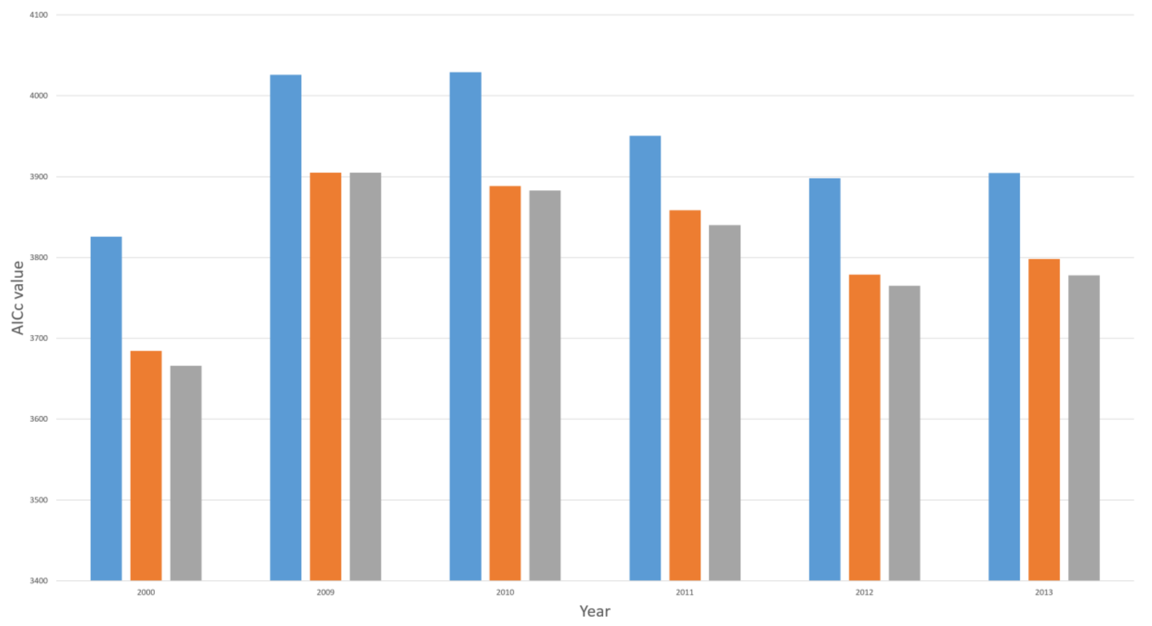
| AIC | 3825.92 | 4029.05 | 4025.85 | 3950.59 | 3897.81 | 3904.38 |
| Adjusted R2 | 0.71 | 0.73 | 0.64 | 0.65 | 0.67 | 0.66 |
| Decennial Census Years | ACS Years | |||||
|---|---|---|---|---|---|---|
| Year | 2000 | 2010 | 2009 | 2011 | 2012 | 2013 |
| Bandwidth | 84 | 98 | 98 | 91 | 77 | 90 |
| RSS | 531,883.1 | 111,8276 | 1,166,110 | 951,077.8 | 633,734.2 | 786,608.1 |
| AIC | 3684.43 | 3888.25 | 3904.78 | 3858.53 | 3778.99 | 3798.11 |
| Adjusted R2 | 0.86 | 0.81 | 0.80 | 0.79 | 0.84 | 0.81 |
| Decennial Census Years | ACS Years | |||||
|---|---|---|---|---|---|---|
| Year | 2000 | 2010 | 2009 | 2011 | 2012 | 2013 |
| Bandwidth | 84 | 98 | 98 | 84 | 77 | 90 |
| RSS | 635,797 | 1,402,213 | 1,479,242 | 1,188,077 | 944,864 | 922,170 |
| AIC | 3666 | 3883 | 3905 | 3840 | 3765 | 3778 |
© 2018 by the authors. Licensee MDPI, Basel, Switzerland. This article is an open access article distributed under the terms and conditions of the Creative Commons Attribution (CC BY) license (http://creativecommons.org/licenses/by/4.0/).
Share and Cite
Ma, Y.; Gopal, S. Geographically Weighted Regression Models in Estimating Median Home Prices in Towns of Massachusetts Based on an Urban Sustainability Framework. Sustainability 2018, 10, 1026. https://0-doi-org.brum.beds.ac.uk/10.3390/su10041026
Ma Y, Gopal S. Geographically Weighted Regression Models in Estimating Median Home Prices in Towns of Massachusetts Based on an Urban Sustainability Framework. Sustainability. 2018; 10(4):1026. https://0-doi-org.brum.beds.ac.uk/10.3390/su10041026
Chicago/Turabian StyleMa, Yaxiong, and Sucharita Gopal. 2018. "Geographically Weighted Regression Models in Estimating Median Home Prices in Towns of Massachusetts Based on an Urban Sustainability Framework" Sustainability 10, no. 4: 1026. https://0-doi-org.brum.beds.ac.uk/10.3390/su10041026