Effect of Roads on Ecological Corridors Used for Wildlife Movement in a Natural Heritage Site


1
Xinjiang Institute of Ecology and Geography, CAS, Urumqi 830011, China
2
Department of Economics, Xinjiang University of Finance & Economics, Urumqi 830012, China
*
Author to whom correspondence should be addressed.
Sustainability 2018, 10(8), 2725; https://0-doi-org.brum.beds.ac.uk/10.3390/su10082725
Submission received: 24 May 2018
/
Revised: 13 July 2018
/
Accepted: 27 July 2018
/
Published: 2 August 2018
(This article belongs to the Special Issue Sustainable Heritage Management)
Abstract
:Roads are the link between geographic space and human socio-economic activities, promoting local economic development, and simultaneously causing various negative effects, such as segmentation, interference, destruction, degradation, and pollution. In China, the construction of roads is rapid, which might affect wildlife movement, landscape pattern, and land use change, thereby, affecting the conservation of heritage sites. In the present study, the minimum cumulative resistance model, along with geographic information system technology, was adopted to compute the ecological corridor for wildlife movement between the source patches and to analyze ecological corridor changes under two conditions (road presence/absence) at two time points in Kanas, nominated as a World Natural Heritage site. The relationships between the ecological corridor changes and various factors, including the cutting index of the ‘road-effect zones’, terrain, and road geometric characteristics, were examined using the geographical detector model to identify the influencing factors and mechanisms of the corridor changes, in order to rationally simulate the potential ecological corridors. In addition, the detached and fragmented ecological patches can be connected to effectively protect the biodiversity, biological habitats, and species, which are important means to achieve regional sustainable development and ecological construction.
1. Introduction
Currently, fragmentation has become a global issue, and anthropogenic activities are considered to be the main cause, especially for the loss of connectivity between different habitats [1]. With the rapid development of the economy, the construction of roads is considered to be one of the main reasons for biodiversity loss, and it is also known as a barrier for wildlife movements [2,3]. It has been reported that the mean road density of the United States is 0.75 km/km2; for Germany, France, and England it is >1.88 km/km2; and for Japan it is >3 km/km2 [4]. Therefore, road construction has become a global problem affecting the environment.
Roads play an important role in socio-economic development, such as connecting geographical space and human socio-economic activities, promoting local economic development, and growing social wealth. However, they also have a direct or indirect effect on the ecosystem, causing various adverse effects on natural landscapes [5]. The effect of roads is reflected by the fragmentation of wildlife habitats [6,7,8], which disrupts the horizontal ecological flow, leading to a series of changes in the ecological processes that affect and alter the structure and process of ecosystems [9].
Similarly, the road type, width [10], and fence [11], and their mixed effect might result in a fragmented wildlife habitat, disconnected wildlife, and, most critically, isolated populations. It has been shown that the width of the road affects the number of wildlife that pass over the road [12]. Furthermore, a road fence might isolate individuals of the same species, or even trap them within the fenced corridor [13,14]. Moreover, during the movement of wildlife, high-speed and high-volume traffic would increase the mortality of small and medium body-sized animals and would fragment the habitat of large animals.
Several studies have shown that the construction of lines and strips (e.g., railways and expressways), and areas affected by roads, named ‘road-effect zones’, might affect land use, soil erosion, vegetation, landscape pattern, habitat or landscape connectivity, ecological risk, animal migration, wildlife corridor, and ecosystems. They can serve as obstacles to separate different parts of landscape, acting as a barrier and filter for wildlife [3,15]. They are also important as wildlife corridors to connect natural areas, allowing wildlife movement, although this depends significantly on the width of the undisturbed native vegetation along the verges.
In the process of protecting the wildlife, the establishment of national parks and conservation reserves is an important means to protect the remaining habitats of wildlife, and are important for the native flora and fauna. Currently, the number of national parks in the United States, Canada, New Zealand, and Australia is 55, 39, 14, and 516, respectively. By the end of 2016, the number of national nature reserves in China was 447, which are separated from each other, and the species in them are also isolated. The islanding phenomenon has become increasingly apparent, leading to a decrease in the species migration rate and an increase in mortality, and consequently, there has been an overall reduction of biology. Therefore, it is commonly believed that the establishment of ecological corridors between nature reserves can connect isolated habitats and reduce the rate of species extinction. Several studies have shown that the paths for wildlife movement can be defined as ecological corridors [16]. There are various benefits of building ecological corridors; for example, protecting the diversity of species, diffusing the animals [17], increasing the exchange of genes, and reducing the risk of extinction [18]. An ecological corridor is the key to the movement and reproduction of wildlife [19]. Whereas other studies have argued that an ecological corridor might provide a channel for the spread of harmful organisms, which is a disadvantage to the survival and spread of the target animals [20]. It also provides a convenient channel for invasive species, predators, pests, and diseases, which could not have spread originally [21]. Furthermore, it can also increase the rate of invasion.
In studies on the identification of the ecological corridor, the theories of island biology and meta-population have usually been suggested as the theoretical foundation. The structure of the ecological corridor refers to the combination of number, background, width, degree of connectivity, composition, and characteristics of key points [22]. Forman (1995) suggested that corridors can be the habitat of the wildlife, and they can act as a channel, source, sink, obstruction, and filter for biological movement [23].
The methods of ecological corridor identification include field observation, a combination of remote sensing (RS) and geographic information system (GIS), reference quantitative research method of landscape pattern, and ecological security [24]. With the development of RS technology, the combination of RS and GIS methods, and the use of the minimum consumption model (least-cost path analysis [LCP]) to quantitatively study the ecological corridor are widely used in corridor identification, ecological network construction, and species management. Among them, the minimum cumulative resistance (MCR) model is a derivation model of the distance-consuming model, which has practical significance in dealing with ecological and geographic factors, and can solve several problems related to the path. In the application of a concrete model, problems such as source patches and resistance surface should be considered. Studies on the ecological corridor have put forward the principle and procedure of corridor design for corridor management, transforming it from theoretical research to a practical application development [25].
Currently, the national highway network approximately 400,000 km in length consists of national highways and ordinary national roads. There are 36 national highways with a total length of 118,000 km, and 200 ordinary national roads with a total length of 265,000 km. Under different administrative standards, the government has different emphases and solutions on road construction in China. The national scale road network planning focuses on the rational layout of road network construction, functional integrity, extensive coverage, and safety reliability [26]. The goal is to achieve high connectivity among core cities, provincial multi-line connectivity, high-speed access to cities and counties, and county–state road coverage. Road construction should consider environmental protection, fully making use of existing routes and avoiding environmentally sensitive areas and ecologically fragile areas.
Road network planning at the scale of provincial and autonomous regions focuses on the establishment of a comprehensive transport system in the region, including a rural road network, urban transport network, and freight logistics network [27]. The goal is to continuously improve and guarantee the economic development of the region, improve the access rate to township and administrative villages, implement processes mainly through the use of existing routes, and implement greening or engineering facilities to eliminate road damage to natural landscapes.
The construction of the road network from the perspective of the local government is to develop an agriculture infrastructure and rural economy. The aim is to satisfy the demands of the local residents, and also to ensure the improvement of rural economic activities and the normal operation of agricultural production. Because of the lack of upper road network planning, the road network construction affects the ecological environment, with pollution damaging the natural environment during the construction and destruction of highways surrounding the ecosystems.
The construction of roads in Kanas is done by the local government. During the late 1990s, as there was an increase in the number of tourists, the local government and the Government of Xinjiang Uygur Autonomous Region increased the funding for the construction of a tourist transportation system to Kanas. Since then, the construction of highways among some villages had been completed. The construction of these highways is of great convenience for tourists to access the scenic spots and has spurred a significant increase in the number of tourists visiting Kanas, thereby, improving the income level of the local residents. However, highway construction has destroyed the integrity of the elite scenery of Kanas, generating an intensive splitting effect on the landscape, and splitting the natural habitats into isolated blocks, forming biological isolated islands, resulting in fragile ecological environment, which might lead to new geological disasters or potential hazards. In this milieu, it is particularly necessary to establish ecological corridors to connect the isolated habitats.
In the present study, we evaluated the effect of roads on the ecological corridors for wildlife movement in Kanas. We attempted to (1) explore the cutting effect of ‘road-zones effect’ on the Kanas landscape; (2) establish the ecological corridor for wildlife movement using the MCR model; and (3) detect the relationship between the changes in the ecological corridor and the road cutting effect, and the geometric characteristics of the road and terrain, in order to enrich and expand the research methods to assess the influence of roads on ecological corridors and to offer suggestions for the construction of a transportation system for the future, in order to reduce the disturbance to the wildlife.
2. Materials and Methods
2.1. Study Area
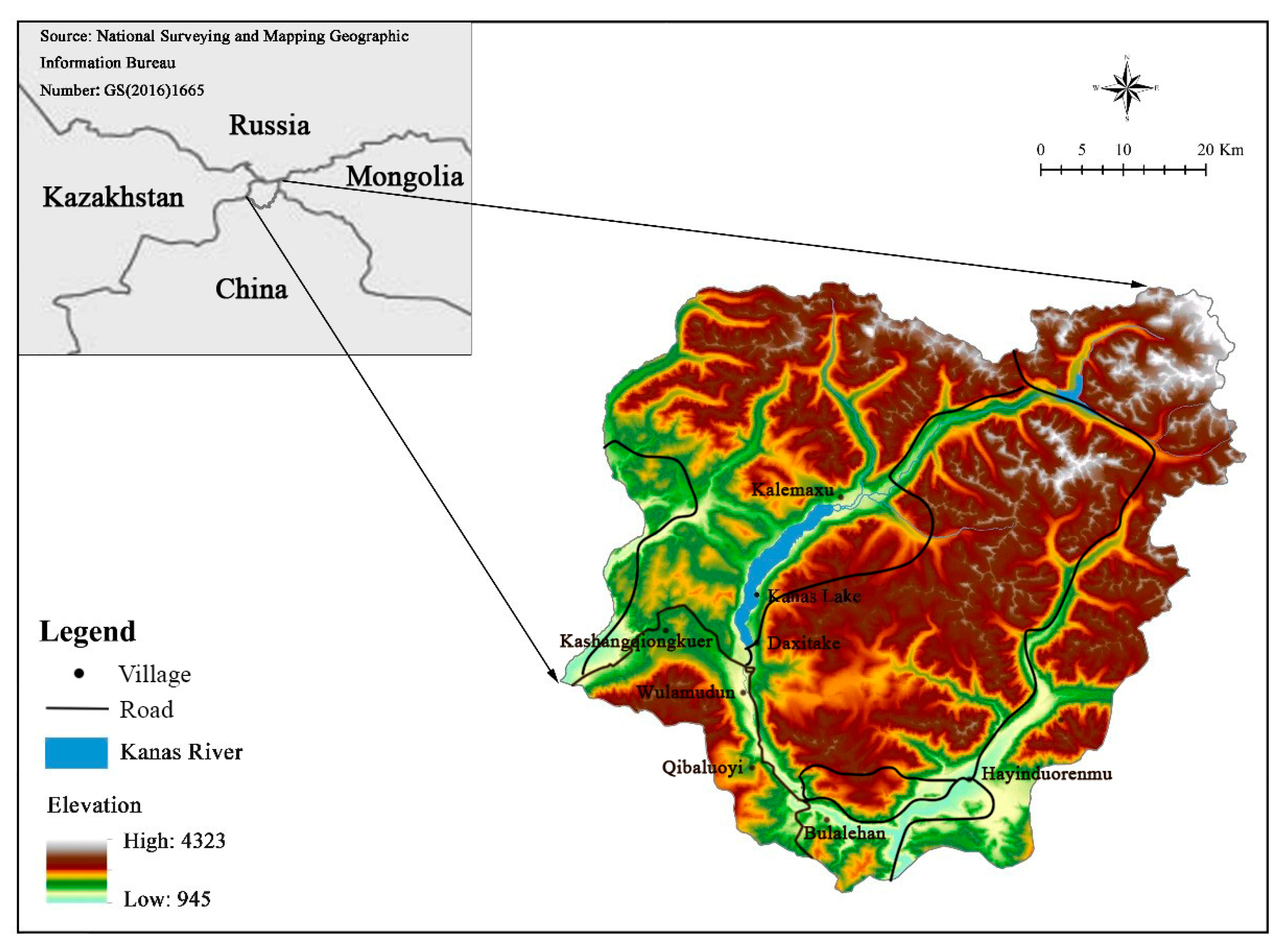
Kanas, nominated as a World Natural Heritage site, was used as the present study area. The site is located at the junction of four countries—China, Kazakhstan, Russia, and Mongolia—along the southern slope of the Altai Mountains and north of Burqin County, with an area of 3194.69 km2. The entire terrain of this area is high in the north and low in the south, with an elevation of 1296–4374 m. The site lies in the cold and temperate zones of the hinterland of the Eurasian Continent, and it has a continental climate, with a warm spring and autumn, cold winter, no summer, and abundant rainfall throughout the year. As a result of the complex topography and significant altitudinal differences, the site has different climatic conditions in different terrains and heights, with six vertical natural zones from low to high altitude that comprise 7 vegetation types, 14 vegetation subtypes, and 43 groups, as well as 361 species of vertebrates belonging 31 orders and 67 families, with the southern slope of Altai Mountains possessing the most abundant species. This site is the only national nature reserve in China that is located at the junction of four countries, and it contains the ‘Altai-Sayan Mountain forest biota’ in China. It is one of the World Wildlife Fund’s ‘Global 200’ key and priority regions for biodiversity conservation, with important protection and research value. It was inducted into the ‘Directory of China’s National Nature Heritage Reserves’ in 2008 (Figure 1).
2.2. Data Sources and Data Processing
In the present study, we used an array of data, including remote sensing images and digital elevation, road vector, soil, hydrology, and vegetation data of the study area. The remote sensing data were collected from September 2000 to September 2013, using the Landsat ETM image data with a resolution of 30 m (Data from http://glovis.usgs.gov/). These remote sensing data were processed using the ENVI 5.0 image processing software, and with reference to the national land use classification system, the landscape was categorized into the following types: forestland, grassland, beach land, bare exposed rock or gravel, glacier and perennial snowfield, and construction land.
The vegetation coverage was calculated using the normalized difference vegetation index (NDVI), as follows:
where, NIR and VIS are the reflectance values at the near-infrared wavelength band and the red wavelength band, respectively; NDVImax is the maximum vegetation index value of the forestland with vegetation coverage; and NDVImin is the minimum vegetation index value of bare exposed rock or gravel without vegetation coverage, in which the vegetation coverage indices are binarized [28,29].
NDVI = (NIR − VIS)/(NIR + VIS)
Vegetation coverage = (NDVI − NDVImin)/(NDVImax − NDVImin)
The digital elevation model (DEM) data with a resolution 30 m were obtained from the Geographic Data Cloud. The road data were divided into three levels, namely, provincial, county, and scenic area. The data on the soils, hydrology, and vegetation were from the Heritage Application Form of the Altai Mountains of Xinjiang, the Physical Geography of Arid Areas in China, and the China Vegetation Map, respectively.
2.3. Research Methods
The research steps are as follows: ① study the physical cutting effect of the ‘road-effect zones’ on the type of landscape; ② study the changes in the ecological corridor of wildlife movement under two conditions (presence/absence of road); and ③ analyze the reasons for the changes in the ecological corridor.
2.3.1. Analysis of the Cutting Effect of ‘Road-Effect Zones’ on the Landscape
• Analysis of road buffering area
Road construction results in varying degrees of interference on the landscape structure and ecological factors in the surrounding areas, with an affected range of at least 100 m and an average interference range of approximately 600 m [3,30]. According to the ‘Highway Law of the People’s Republic’, the roads were divided into national, provincial, county, and rural roads. In this context, the road buffering range of the study area was defined as the ‘road-effect zones’. According to the road type, the radius of the ‘road-effect zones’ around the provincial, county, and rural roads was set at 500, 100, and 50 m, respectively [31].
• Determining the cutting index of the ‘road-effect zones’
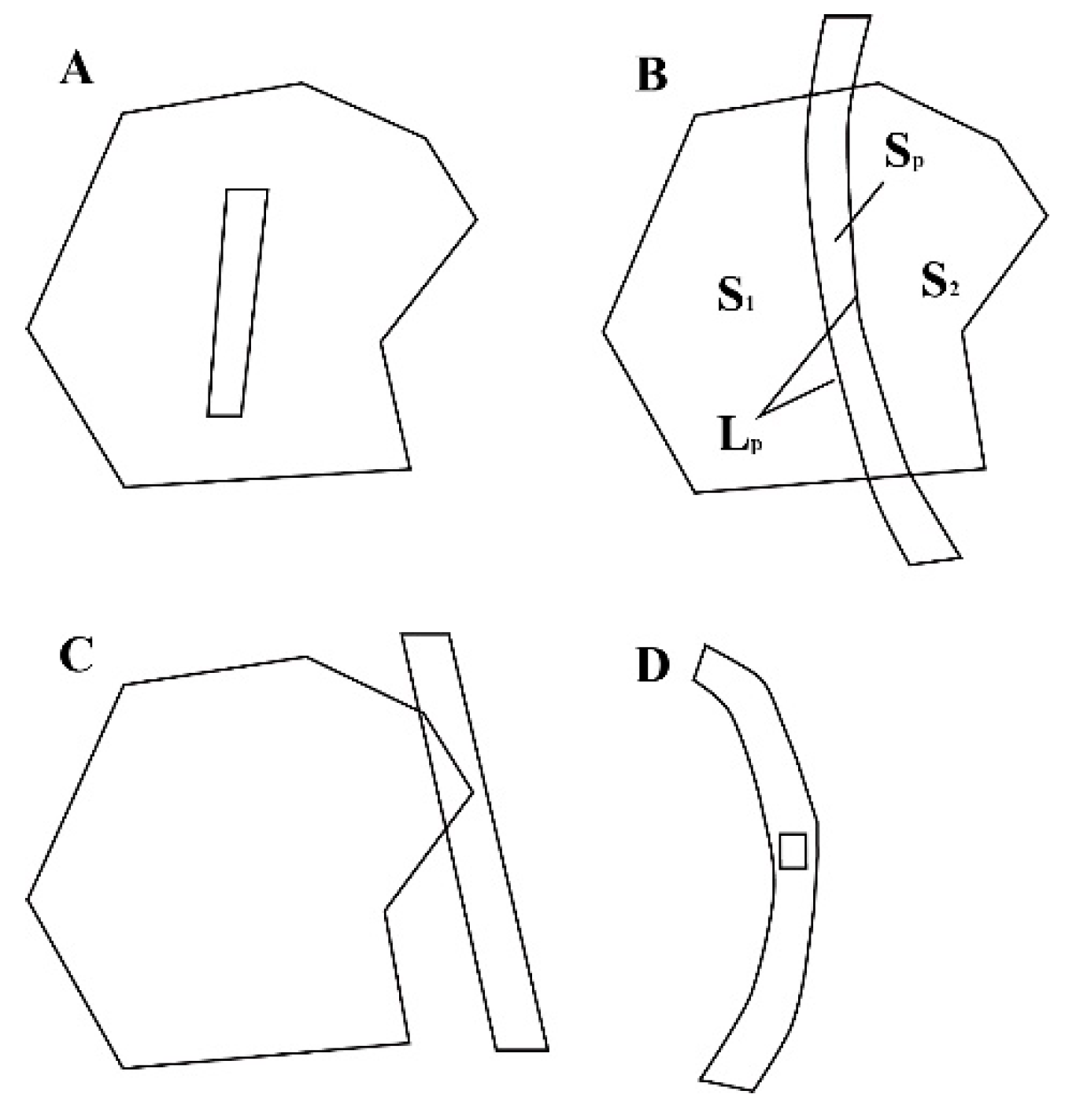
Corridors, as linear landscape units, play a dual role as both the path and barrier for material movement or flow [32]. In the present study, different road levels in the above set up of the buffer zone as ‘road-effect zones’ exhibited a significant cutting effect on the landscape. The cutting function of the ‘road-effect zones’ on landscape patches can be divided into four modes, that is, complete cutting, middle cutting, internal cutting, and edge cutting modes [24]. The complete cutting mode can be defined as the zones of the road-effect, including all of the patches that have a negative effect on the original patches, and therefore, have the largest effect on ecological conservation. The middle cutting mode can be defined as the original patches divided into two pieces, and therefore, the landscape is fragmented, blocking the internal material and energy flow between the original patches; it has a relatively high effect on ecological conservation. The internal cutting mode can be defined as the ‘road-effect zones’ in the original patches, with a filling expansion in the original plaque; the increase in the source of the risk leads to an increase in the distance of the material and energy flow between the original patches, and the ecological influence is moderate. The edge cutting mode can be defined as the ‘road-effect zones’ only encroached in the most outer area of the original patches, and the ecological effect is small; the adjacent edge length is the sum of the sides of the ‘road-effect zones’ and the cut patches (Figure 2).
Figure 2A is the internal cutting mode, the ‘road-effect zones’ in the original patches, forming a filling expansion. Figure 2B is the middle cutting mode, the ‘road-effect zones’ divides the original patches into two pieces; Figure 2C is the edge cutting mode, the ‘road-effect zones’ edge only invades the outer area of the original patches; Figure 2D is the complete cutting mode, the ‘road-effect zones’ contain all of the patches; Sp is the area of the patch occupied by the ‘road-effect zones’; S1 is the area of the left patch after the middle cutting; S2 is the area of the right patch after middle cutting; and Lp is the adjacent length between the corridor and the cut patch.
The direct influence of the ‘road-effect zones’ project on patch cutting is landscape encroachment and neighboring interference. Landscape encroachment can change the land use pattern, and the different landscape types have a different influence on the natural ecological environment and their own ability to maintain a natural equilibrium state [33]. The neighboring interference can change the adjacency compatibility coefficient of the ecosystem elements, resulting in changes in the ecological material consumption and energy flow [34]. The ’road-effect zones’ to cut the pattern of patches, occupied areas, and adjacent edge length can be used to determine the cutting index; the larger the occupied area and longer the adjacent edge, the higher the effect on the cutting patches.
The formula is as follows:
where, CCIi is the degree of the ‘road-effect zones’ cutting in the ith type of landscape; Sij is the area of the jth cut patch in the ith type of landscape; Lij is the length of sides of the jth cut patch in the ith type of landscape; Sijp is the occupied area of the ‘road-effect zones’ in the jth cut patch of the ith type of landscape; Lijp is the length of the adjoining sides of the ‘road-effect zones’ after it occupies the jth cut patch in the ith type of landscape; S is the total area of the study area; W is the impact index of cutting mode, of which the indices of the edge cutting, internal cutting, middle cutting, and complete cutting modes were set to 1, 3, 5, and 7, respectively; and m is the total number of cutting of the ‘road-effect zones’ in the ith type of landscape [35].
2.3.2. Research Method to Determine the Ecological Corridor for Wildlife Movement
The minimum cumulative resistance model (MCR) refers to the sum of resistance that is overcome by reaching the target point from the ‘source’, through different resistance units. In nature, the movement is influenced by resistance; the less the resistance, the easier the flow. It also shows that the region has a relatively perfect and reasonable ecological structure. Unlike the traditional spatial model, the resistance identified by the MCR model is not the actual distance between the points, but the coefficient of the depletion of the material and energy flow within the unit during the passage, that is, the difficulty of traversing the unit.
The MCR model reflects the landscape resistance of the different landscape matrixes to space motion. The friction coefficient of each unit moving past an object or a phenomenon is calculated by determining the cumulative coefficient of matter and energy on different surfaces, to represent the cumulative resistance that a species needs to overcome in order to pass a heterogeneous landscape, determined using the following formula [36]:
where the MCR is the minimum cumulative resistance of the matter or energy from the origin to a point in space, which is related to distance and cost; f is a monotonically increasing function, which reflects a positive proportional relationship between the MCR and the variable (Dij × Ri); Dij represents the material and energy flow from the i source unit to the j unit in the motion path after leaving the source, the motion distance when unit i is passed; and Ri represents the resistance coefficient of the i unit to motion [37].
In the present study, we used the GIS Arcgis10.5 to calculate the path of MCR, which is the ecological corridor for wildlife movement in the study area in 2000 and 2013. It is necessary to consider three aspects in the process, including the factors of the source patch, motion distance, and surface space characteristics.
• Selection of source patch for wildlife movement
The establishment of an ecological corridor is used to maintain and improve the landscape of the research area. The choice of the ecological source is mainly to maintain and improve the region by establishing the relationship with other components [38]. The selected source patches were in the southern most edge of Siberia, Taiga, which is the distribution area of the Siberian pine, and rare and endemic species of the area, such as Abies sibirica, Larix sibirica Ldb., Juniperus sabina L., Sorex asper, and Canis lupus, which have ecological significance [39]. The area of the forest landscape occupies the entire study area; the area is large and has good connectivity. The area also has several wild animals, including rare and endangered animals. Furthermore, the region plays an important ecological role in the entire Kanas estate nominated land, and therefore, was chosen as the ecological source point in the present study. According to the 2000 and 2013 land use classification of the study area, 9 and 29 blocks (each of area >1 km2) were selected, respectively, as the output source patches for species migration.
• Determination of wildlife movement surface resistance
The determination of the resistance coefficient is the key to the rationality of the whole analysis result; however, there is no accepted method and model to determine the resistance coefficient.
According to previous studies, the topographic factors directly affect the distribution and migration of the wild animals, and will affect the construction of the corridors, depending on the habitat suitability of the species. The elevation and slope factors are divided into five levels, and the elevation of >3000 m and slope of >40° were defined as the binding conditions, which had little movement here [40,41]. It is considered that this kind of habitat is not suitable for the survival and movement of most species.
Vegetation coverage directly affects the food acquisition of wild animals, and it is treated as two values, as follows: assuming that the vegetation-covered area is suitable for the survival and movement of most species, the coefficient of resistance was set as 1; and if the vegetation-free area is not suitable for the survival and movement of most species, the resistance coefficient was set as 100.
The soil types affect the productivity of the vegetation and have a certain influence on the vegetation coverage, thus, indirectly affecting the food acquisition of the wildlife. According to the differences in the productivity of the different soil types, the resistance coefficient of the different soil types was set based on previous studies.
The migration of wildlife is influenced by topography, vegetation coverage, and human factors [42]. In the present study, the difference in the degree of human disturbance is differentiated according to the land-use type, and the resistance value of the land-use type was determined according to the intensity of the human disturbance, availability of wild animals, and vegetation coverage degree [43]. Considering that the degree of vegetation cover of the woodland is relatively large in the study area, if the passing by wild animals is high and the human disturbance degree is low, the resistance value was set as 1. If the vegetation cover of the construction land was small and the human disturbance degree was high, the resistance value was set as 800. The resistance value of the other types of landscape were assigned based on that of similar research areas of other studies.
As a man-made creation, roads have the characteristics of high human disturbance and small vegetation cover, and the accessibility for wildlife is low. According to the different types of road, considering their influence range, the resistance coefficient was set; among which, the resistance coefficient of the provincial road was the highest and that of the rural road was the lowest.
In the final determination, the resistance coefficient was set as 1 if the roads type has a good wildlife passing and high vegetation cover; the resistance coefficient was set as 1000 if the type was the most difficult to pass by the wild animals. The vegetation coverage average coefficient was low, and the human disturbance average coefficient was large; and the other types resistance coefficient were moderate. In this study, we neglected the resistance separation of the different species to the specific resistance factors when they are moving (Table 1).
From the assigned weights, the resistance images, including the elevation, slope, soil type, vegetation coverage, and land-use type for each parameter were generated. The statistical weight was calculated using the hierarchical method analytic hierarchy process (AHP), proposed by Saaty (1977) [46]. The AHP is a multi-criteria decision method to determine the relative weight of the different factors in the model (Table 2).
The weight of the resistance factors was set to 0.0337, 0.0725, 0.1499, 0.2191, and 0.5247, respectively, which passed the consistency test with a value of 0.0420 (<0.1).
Given the resistance images of each parameter and their respective statistical weights, we obtained the total resistance image, using the following equation:
where, Total Resistance is the total resistance image, elevation resistance is the resistance image of elevation, slope resistance is the resistance image of slope, soil-type resistance is the resistance image of soil type, vegetation coverage resistance is the resistance image of vegetation coverage, and land-use type resistance is the resistance image of land use type.
Total Resistance = 0.0337 elevation resistance + 0.0725 slope resistance + 0.1499 soil-type resistance + 0.2191 vegetation-coverage resistance + 0.5247 land-use type resistance.
• Extraction of optimal ecological corridor for wildlife movement
We assumed that the path of the minimum cumulative resistance value is preferred when the wildlife is moving and spreading. Using the spatial analyst module of ARCGIS 10.5, the minimum cumulative resistance path was calculated. Firstly, using the reclassify tool to classify the resistance factor into the grid data, the cumulative resistance surface was calculated using the Raster calculator tool. Finally, the optimal path was obtained using the cost weighted and shortest path tools [47,48] (Figure 3).
2.3.3. Determination of the Factors Responsible for the Changes in the Ecological Corridor
The geo-detector model was used to determine the spatial differences among the geographical elements; it is an independent model to analyze the driving force and to influence the factors of various phenomena and the interaction between multiple factors [49].
The determination of the variation and its factors is as follows: the spatial variation of Y, as well as the extent to which factor X explains the spatial variation of attribute Y was detected using the following formula:
where q is the index of the detection power for the spatial variation of dependent variable; when h = 1, …, L is the stratification of variables or factors (i.e., categories or regions); Nh is the number of sample units in sub-regions; N is the number of sample units in the entire region; L is the number of sub-regions; σ2 is the variance of the dependent variable of the entire region; and σh2 is the variance of the sub-regions [50].
The detection of interaction will help identify the interactions among the different factors. That is, to evaluate whether the presence of an interaction between the factors strengthens or weakens the explanatory power of the dependent variable, or whether the influence of these factors on the dependent variable are independent of each other. The calculation method is as follows: firstly, the q values (q [X1] and q [X2]) of the factors (X1 and X2) on the dependent variable, and the q value of their interaction (q [X1 ∩ X2]) were calculated, then, q (X1), q (X2), and q (X1 ∩ X2) were compared.
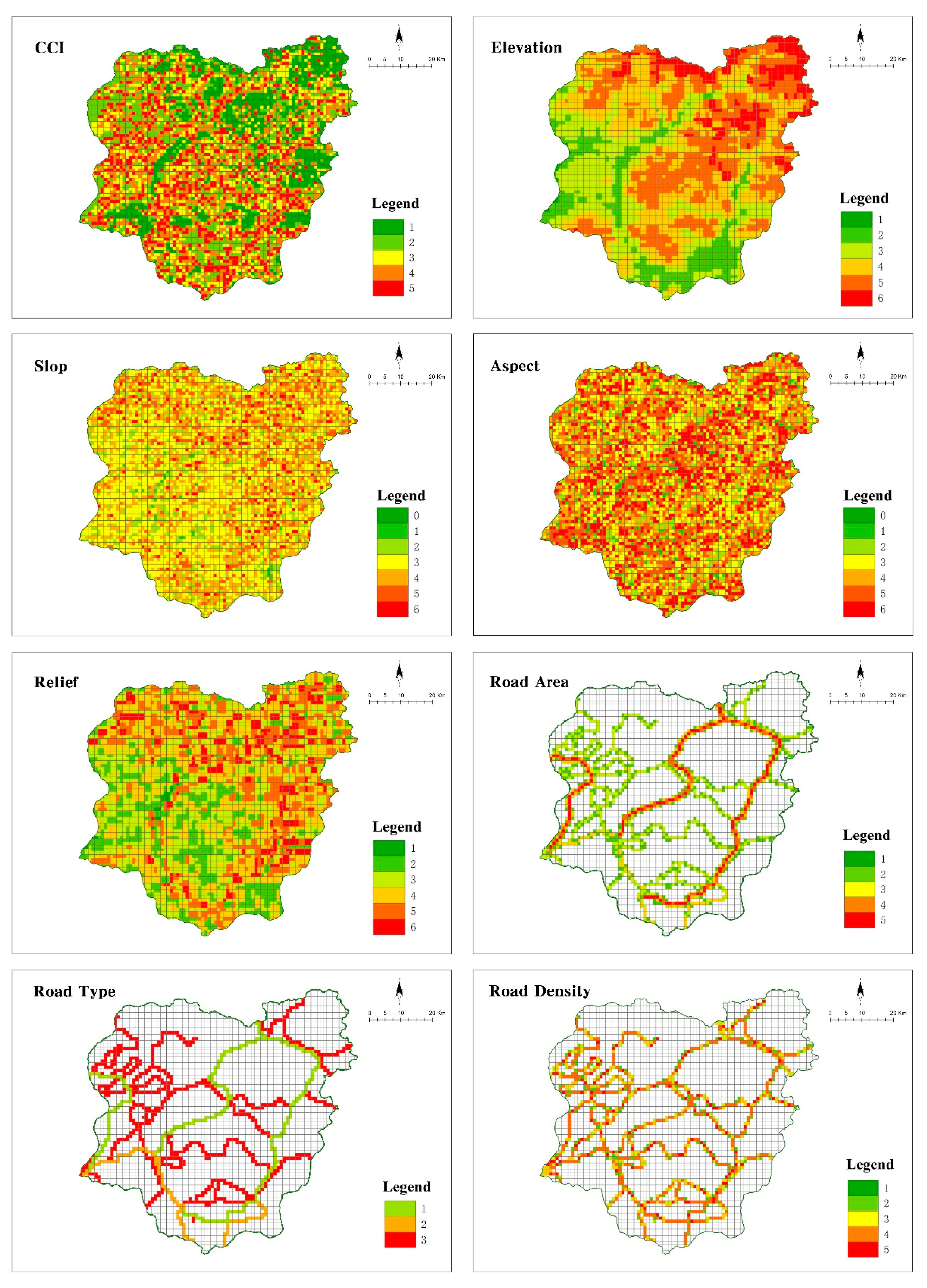
In the application of the model, the following steps were involved: ① the spatial gridding of the study area was carried out by the equidistance method of a 1 km × 1 km scale; ② in 2013, we calculated every central grid with roads and without roads under both of the conditions, the change value of species migration corridor, and the data of road physical cutting, road, terrain, and other factors; ③ using the geographical detectors, we identified the factors that cause changes in the ecological corridor, based on the relationship between the change value of the ecological corridor and road cutting index, road geometric property (road density, road area, and road type), and topographic factors (fluctuation, elevation, slope, and aspect) under both of the conditions. Of which, the data of the geo-detector require the quantity type of the independent variable; therefore, the ‘road-effect zones’ cutting degree, road density, road area, fluctuation, elevation, slope, and aspect value of the above factors were divided by the natural breaks method, and the classification quantity was determined according to the numerical characteristics of the factors. The road types were divided according to the ‘Highway of the People’s Republic’, into national, provincial, and rural roads (Figure 4).
3. Results
3.1. Analysis of Road Cutting Effect of the Study Area
3.1.1. Analysis of the Landscape Pattern in the Road Buffer Zone
According to the classification of roads by the ‘Highway Law of the People’s Republic’, the roads in Kanas included provincial, county, and rural roads. The S232 Provincial Highway and dozens of county roads crisscross the study area. During 2000–2013, the road system in the study area was well developed, because of which, the total length of the roads increased from 332.44 to 901.83 km.
For the buffering analysis of the roads in Kanas, as far as the area of the landscape type is concerned, the area order of the top three landscape types in road buffer was as follows: grassland > forestland > bare land, in 2000–2013. In 2013, the area of each landscape type within the road buffer changed, with the area of grassland serving as the matrix landscape within the road buffer, increasing by 71.27 km2, whereas, that of the forestland reduced by 20.68 km2, and that of the bare land increased by 5.58 km2.
In terms of landscape type, the road buffer area increased the beach land and construction land landscapes, and decreased the glacier landscape in 2013. The reason for the emergence of the beach land and construction land is that the increase in roads increased the road buffer coverage area. Furthermore, during 2000–2013, the study area of the inner elite landscape road buffer near the area of the construction land increased. The reason for the disappearance of the glacier type landscape, on one hand, is that the increased roads are distributed in the low elevation area of the study area; the buffer area does not contain glaciers. On the other hand, because of the retreat of the glaciers, the existing roads containing glaciers disappear. That is, the forestland and grassland account for a large proportion, whether it was 2000 or 2013, and they were still the matrix in the road buffer.
3.1.2. Cutting Effect of ‘Road-Effect Zones’ in the Study Area
The road buffer area was considered as the ‘road-effect zones’, which has cutting effect on the landscape of the study area. During 2000–2013, the cutting modes of the ‘road-effect zones’ on the landscape patches included the edge cutting, middle cutting, and complete cutting modes.
In 2000, the landscape area of the ‘road-effect zones’ under the middle cutting mode was the highest at 574.3 km2. The grassland and forestland had the highest number of middle cutting modes, at 64 and 15 times, with occupied areas of 132.43 and 86.87 km2, and the lengths of the adjoining sides being 535.88 and 363.3 km, respectively. Under the edge cutting mode, at 14.36 km2, the forestland and bare land had the highest number. The landscape area of the ‘road-effect zones’ under the complete cutting mode was the lowest, and the forestland had the highest number. The cutting of the corridor exerted a significant effect, and the landscape types with the highest CCI were as follows: grassland > forestland > glacier > bare ground (Table 3 and Table 4).
In 2013, the landscape area of the ‘road-effect zones’ under the middle cutting mode was still the largest, at 234.8 km2. Grassland and forestland presented the highest number of middle cutting mode, at 19 and 76, respectively, with occupied areas of 193.29 and 40.6 km2, and lengths of adjoining sides of 535.88 and 363.3 km, respectively. In the edge cutting mode, forestland and grassland presented the highest number, at 127 and 27, respectively; with occupied areas of 30.77 and 8.47 km2 and lengths of adjoining sides of 366.75 and 98.53 km, respectively. The landscape area of the ‘road-effect zones’ in the complete cutting mode was the lowest, and the landscape types affected by the complete cutting included forestland, grassland, and construction land, and the landscape types with the highest CCI were as follows: grassland > forestland > bare rock > beach land > construction land. See Table 5.
During 2000–2013, the cutting time of landscape types, except that of the grassland, within ‘road-effect zones’ exhibited an upward trend under the edge cutting, middle cutting, and complete cutting modes. The area of forestland within the ‘road-effect zones’ decreased, whereas the times of the edge cutting, middle cutting, and complete cutting modes increased, and the value of CCI decreased. The area of grassland increased, and the time of the edge cutting and complete cutting modes decreased, whereas, that of the middle cutting mode increased and value of CCI increased. The time of cutting in the bare land and construction land increased, whereas, that of the glacier landscape decreased, and the value of CCI presented a negligible overall change.
3.2. Analysis of Ecological Corridors for Wildlife Movement in the Study Area
3.2.1. Resistance of Ecological Corridor for Wildlife Movement
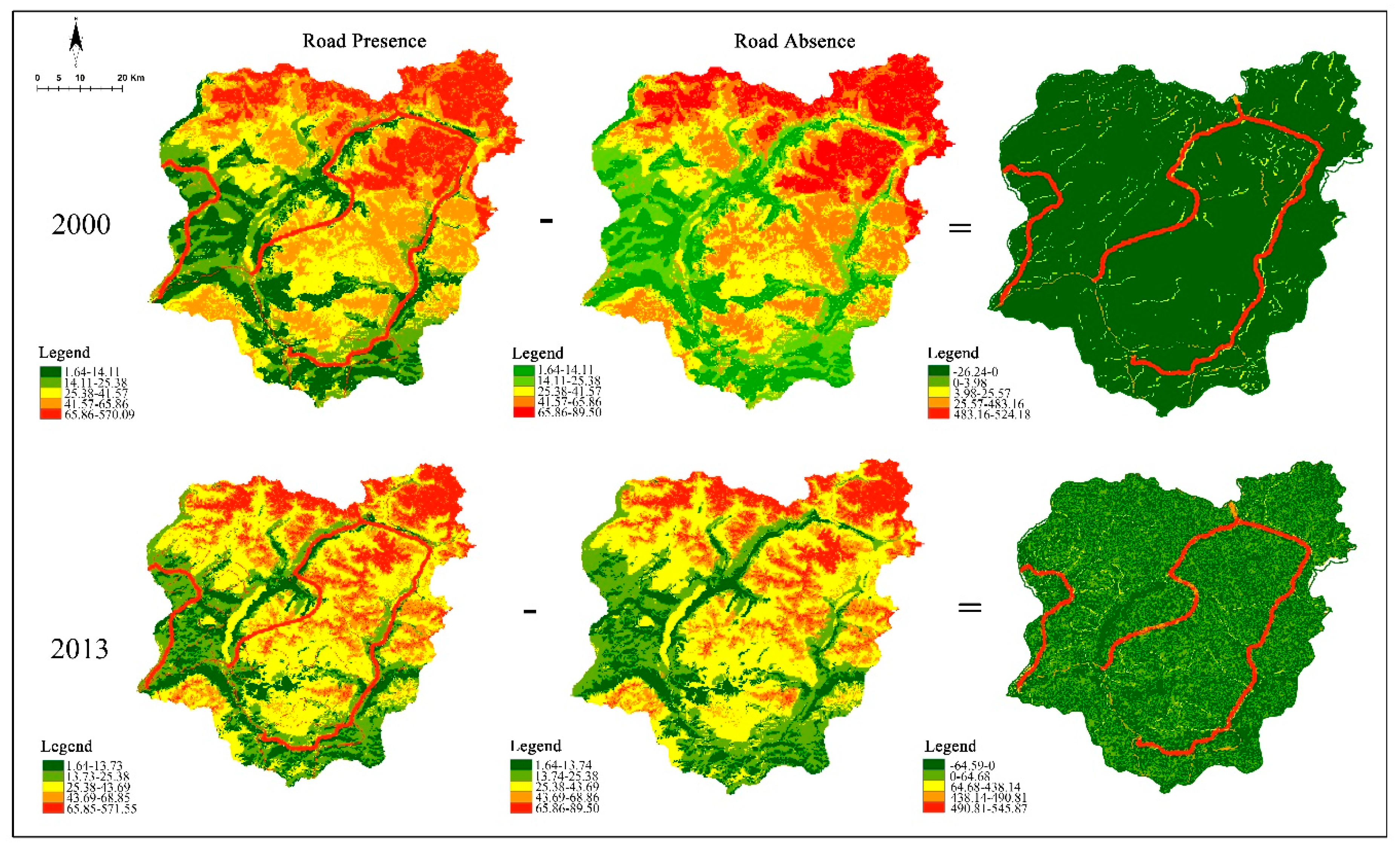
The results of the resistance difference between the two conditions (presence/absence of roads) in 2000 and 2013 revealed red and orange areas, which represent regions with a high resistance value. The emergence of roads increased the resistance value of the areas previously with a low initial resistance value, resulting in the appearance of a circular wall, among the source patches in 2000 and 2013.
During 2000–2013, the range of the resistance values under both of the conditions was similar, but the concentrated distribution areas of the resistance values differed. The areas with altered resistance values concentrated in areas along the road, whereas the resistance values of the roads on the bare land and glacier edge also increased. Specifically, in 2000, the resistance value range under the condition of the absence of roads was 1.64–89.5, whereas that under the condition of the presence of roads was 1.64–570.10. Furthermore, the resistance values under both of the conditions were mostly in the range of 41.57–65.86, accounting for 24.8% and 24.5% of the total area of the study area, respectively. In 2013, the resistance value range under the condition of the absence of roads was 1.64–89.5, whereas that under the condition of the presence of roads was 1.64–570.10. The resistance values under both of the two conditions were mostly in the range of 25.38–43.69, accounting for 36.2% and 35% of the total area of the study area, respectively (Figure 5).
3.2.2. Ecological Corridors for Wildlife Movement
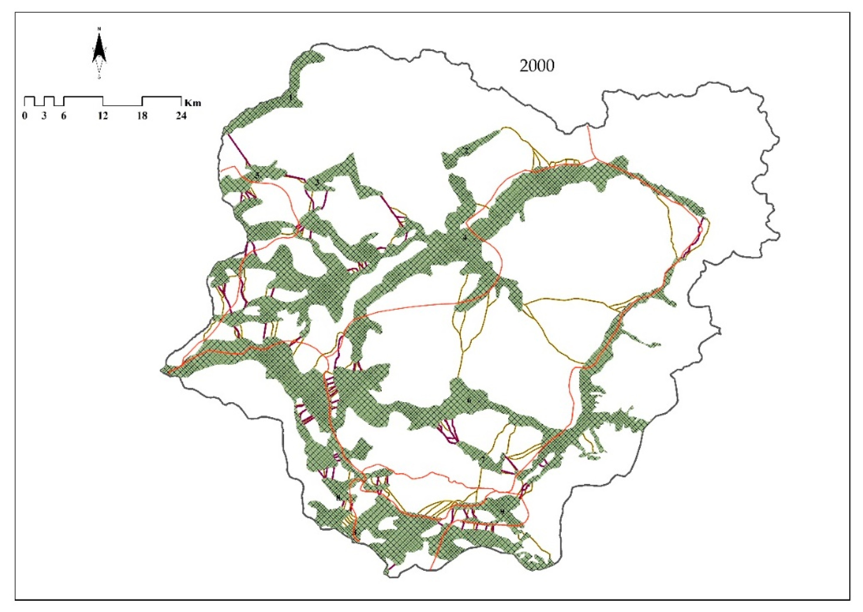
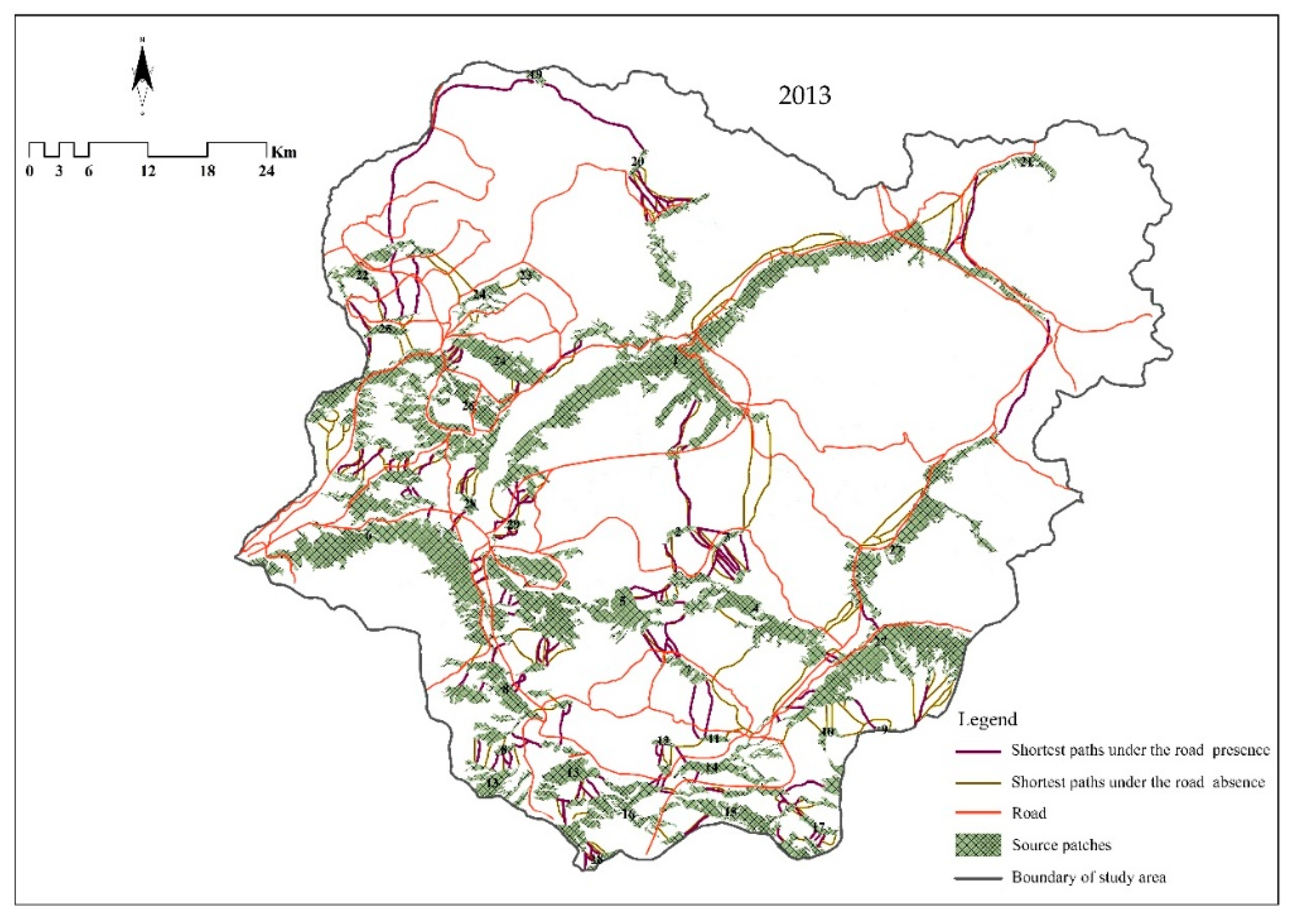
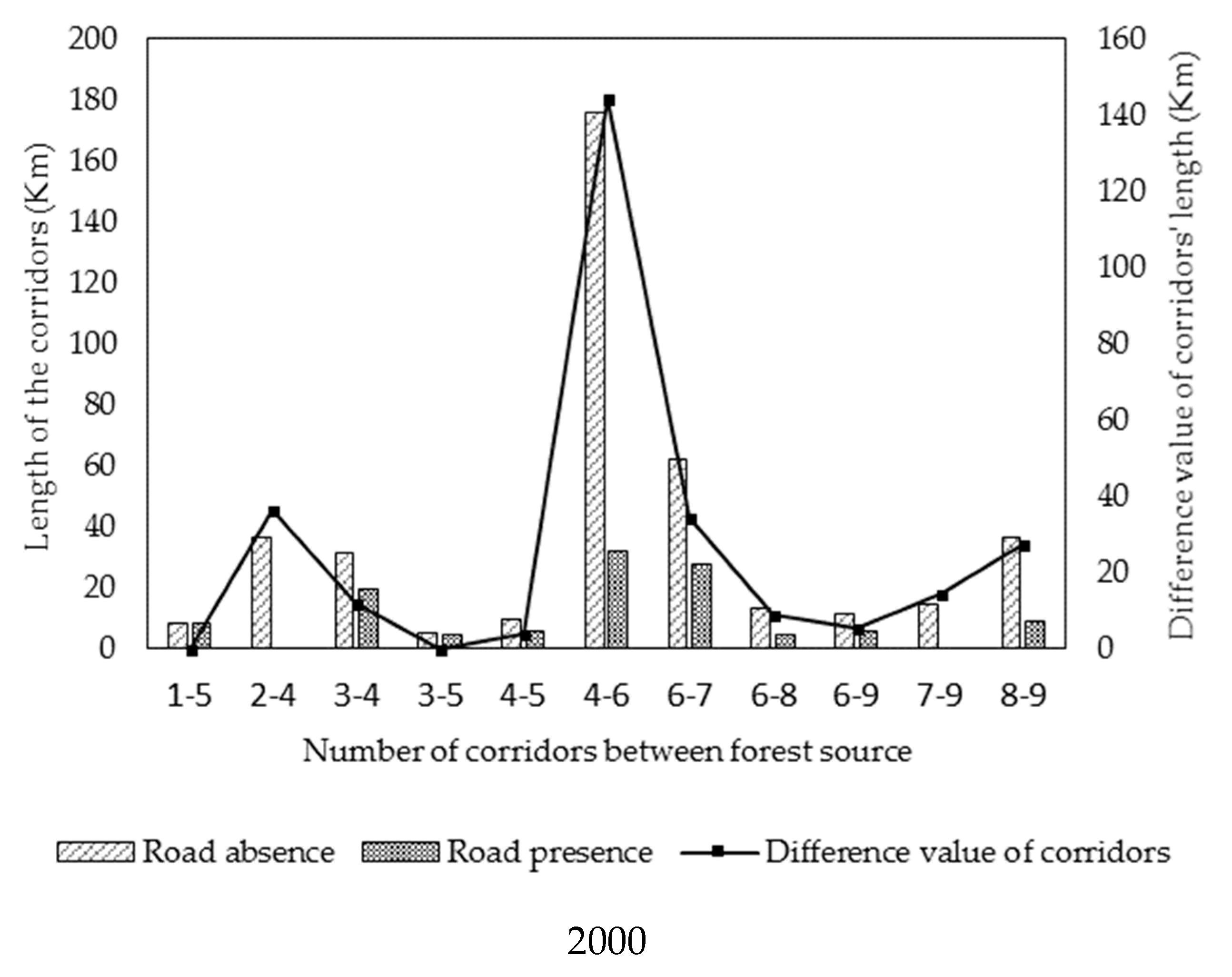
The source patches in 2000 and 2013, were 9 and 29 in the study area, respectively. According to the MCR model, the path between the source patches is defined as the ecological corridor under both of the conditions (presence/absence of roads) in 2000 and 2013.
In 2000, the ecological corridors for wildlife movement in the study area under both of the conditions (presence/absence of roads) differed significantly, manifesting in a decrease in the total number of corridors from 77 to 34, whereas, the total length of the corridors decreased by 229.01 km, and the maximal value of the mean length of corridors decreased from 5.23 to 4.89 km. Under the two conditions, the number and total length of the corridors between patches four and six decreased. The number of corridors decreased from 24 to 7, and the total length of the corridors decreased by 144.12 km. In addition, compared with the distribution of the corridors under the condition of absence of roads, nine corridors between patches 2 and 4 and between patches 7 and 9 disappeared under the condition of presence of roads (Figure 6).
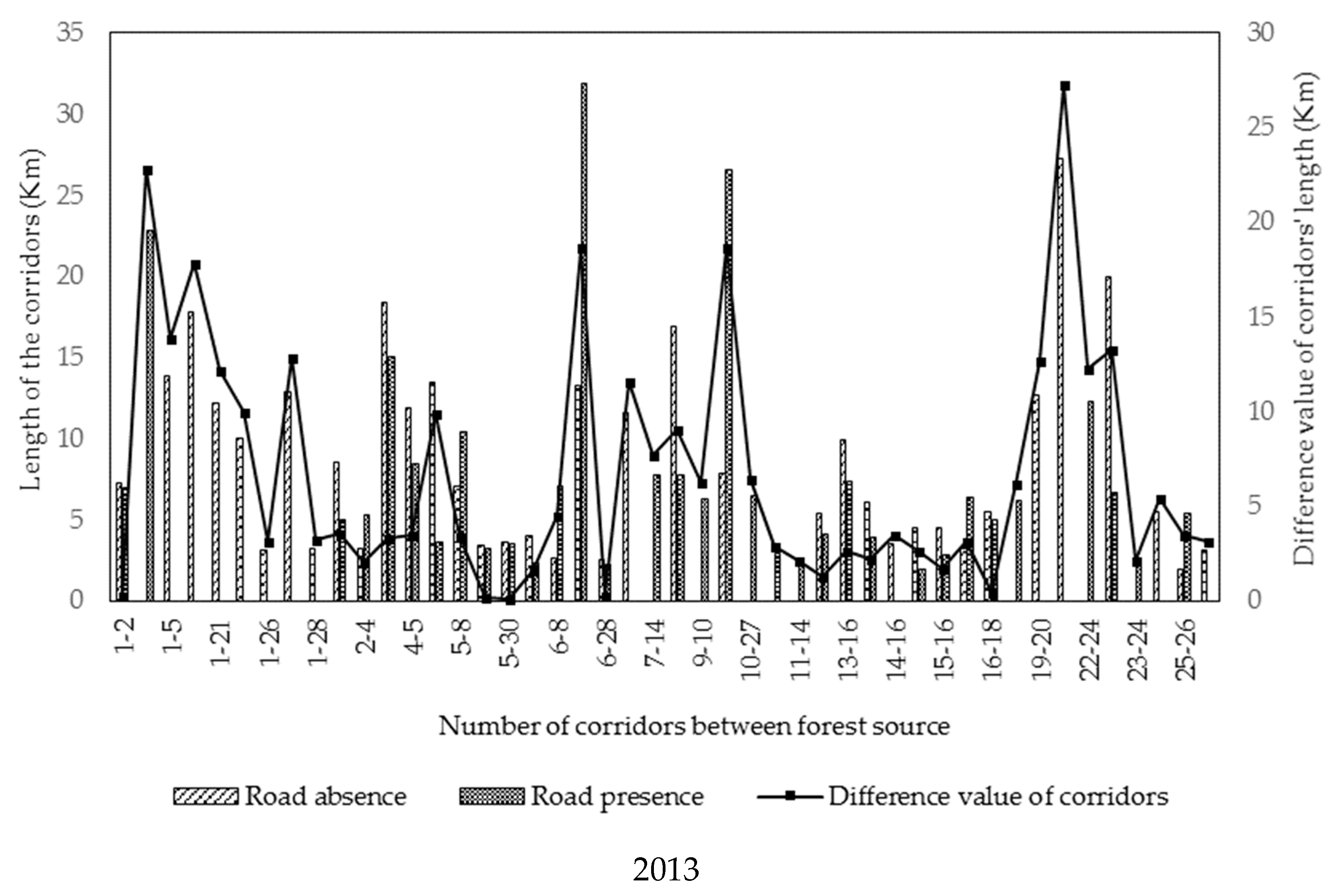
In 2013, under both of the conditions, the total number of ecological corridors for wildlife movement in the study area increased from 109 to 117, the total length of the corridors increased by 37.74 km, and the maximal value of the mean length of corridors increased from 6.09 to 11.39 km. The number of corridors between patches 8 and 13 were approximately 8 in the absence of roads, and the number of corridors between patches 6 and 26 were approximately 14 in the presence of roads (Figure 6).
During 2000–2013, under the condition of the absence of roads, the number of ecological corridors for wildlife movement increased from 77 to 109, whereas, the total length of the corridors decreased by 98.05 km. Under the condition of the presence of roads, the number of ecological corridors for wildlife movement increased from 34 to 117, whereas, the total length of the corridors increased by 227.49 km. Under both of the conditions, the characteristics of the ecological corridor for wildlife movement differed, and in 2000, both the number and total length of the ecological corridors for wildlife movement showed a decreasing trend. Some corridors between patches disappeared under the condition of the presence of roads, and no increase in the corridors between patches was observed. In 2013, the number, total length, and mean length of ecological corridors for wildlife movement under the two conditions showed an increasing trend, and both a disappearance and addition of corridors between the patches were observed.
3.3. Relationship between Detected Factors and the Changes in Ecological Corridor
According to the analysis of the geographical detector, the q values of the detected factors were as follows: CCI (0.0222) > elevation (0.0201) > road area (0.0130) > road type (0.0087) > road density (0.0073) > aspect (0.0040) > relief (0.0015) > slope (0.0009); of which, the q values of the road relief and slope were not significant (Table 6).
Based on the results of the significance test of the geographical detector model, the factors elevation, road area, road type, road density, and aspect were statistically significant with respect to the changes in the ecological corridors, whereas the factors in the relief and slope did not pass the significance test. Therefore, the factors of road density, road area, road type, elevation, aspect, and CCI were chosen to determine the interaction effect on the changes in the ecological corridor, using the geographical detector model (Table 7).
As a function of the geographical detector model, interaction detection is used to evaluate whether the above factors have a common effect on the changes in the ecological corridor, or whether the effect of the above factors on the corridor is independent. The result showed that the interaction effect of any two factors in the above list on the changes in ecological corridors was higher than the effect of one variable alone, and the effect of any two factors on the changes in ecological corridors showed non-linear strengthening or mutual strengthening (Table 6).
The interaction between the factors of CCI and road density, or between the CCI and slope aspect was significantly higher than that of each factor alone, as well as the total of explanatory power of each factor. The results indicated that the effects of CCI, road density, and slope on the changes in the ecological corridor were synergistic. The interaction between the CCI and road area, between the CCI and road type, or between the CCI and elevation was higher than that of each factor alone, but lower than that of the total interaction of each factor. The results indicate that the effect of the CCI, road area, road type, or elevation on the changes in ecological corridors is mutually strengthening. The interaction between elevation and road density, between elevation and road area, between elevation and road type, and between elevation and slope aspect showed synergism. Furthermore, the effect of the interaction of elevation and each of the above factors on the changes in the ecological corridors was significantly higher than that of each factor alone. The effect of the interaction of the road area and the road density or road type on the changes in the ecological corridors was mutually strengthening.
4. Discussion and Conclusions
4.1. Cutting Effect of Road on Landscape
Roads as lines and strips have an obvious cutting effect on the landscape, cutting the entire landscape into isolated patches, causing the fragmentation of landscape, isolation of wildlife, and formation of an island, which can decrease biodiversity. In the zone of ‘road-effect zones’, the landscape type had changed in 2000 and 2013. Beach land and construction land landscapes appeared, and the glacier type landscape disappeared. This is related to anthropogenic activity and climate change. During 2000–2013, the cutting landscape of road construction presented the largest landscape area with an intermediate cutting effect, indicating that ‘road-effect zones’ can produce a large median cutting effect on landscape along the route.
The intermediate cutting effect has the highest influence on grassland and woodland, indicating that it is highly important to protect the grassland and woodland in the environment around the road. As the forestland and grassland are the matrix landscape type of the heritage site, the middle cutting of the patches will hinder the ecological flow within the patches, aggravating the degree of fragmentation of the wildlife habitat and affecting the spread and movement of the wildlife at the individual or population level. The effects of the edge cutting, middle cutting, and complete cutting increase the proportion of the edges and the level of fragmentation of the habitats, affecting the quality of the habitats of wild animals and plants, ecosystems, and landscape patterns in the forestland and grassland, as well as the functioning of ecosystems.
4.2. Methodology of Ecological Corridor for Wildlife Movement
The theories of island biology and meta-population are the basic theories of ecological corridor research. The former suggests that the extinction of wildlife increases if the patch size decreases or the distance increases. Therefore, the diversity of the species would decrease with the cutting effect of roads, increasing the level of fragmentation and the distance of the patch. The latter theory argues that the meta-population is a system of patch populations that consist of two or more sub or local populations, and they are isolated by space, but connected in function. Therefore, increasing the ecological corridors between the fragmentation patch or nature conservation will provide a good channel to find the most suitable habitat for the spread of wildlife, which are isolated from each other because of fragmentation.
Studies on the effect of roads on wildlife movement started in the 1960s, and they mainly focused on the effect of roads on the biological and physical environment [3]. These studies also assessed the influence of geometrical characteristics, including the road type, quantity, traffic volume, speed, and road fence construction, on brown bears, wolves, and other wild animals. In China, studies began to pay attention to the influence of roads on the landscape pattern, land use, and ecological carrying capacity in the 1990s [51,52]. Furthermore, studies on the influence of roads on wildlife have mainly focused on pandas and Asian elephants; in-depth studies on other wildlife are limited.
One of the widely applied models, while choosing a method to build corridors, is the minimum cost model. The least resistance model (as the derivative model of minimum cost model) is often used to build corridors in China. Although the aim of building corridors is similar between China and other countries, that is, to act as a bridge to connect the broken habitat and protect the diversity of wild animals, there are still some differences. The aim of building corridors in other countries is to protect the habitat of specific wildlife. While building corridors, attention would be paid to the genetic characteristics of wildlife, and the source of the corridors is determined by assessing the habitat suitability; food sources, water location, terrain, and other factors are also considered. Whereas studies in China have mainly focused on the regional scale ecological network building and connectivity of a network; for example, they build ecological corridors by studying the habitat suitability of the panda and Asian elephant. However, the Government of China has great executive power and can complete the construction of a biological corridor through policy-oriented mechanism in a short time.
Currently, there are a few studies on the management of biological corridors in China and other countries, and most of them focus on the government’s legal and policy management [53]; a few studies have been conducted with interest in the community residents. Through the study of the corridors of wolves and other wildlife, between Algonquin Park and Adirondack Park in New York, Brown and Harris (2005) [54] found that most people do not trust corridor binding, and only a few people showed interest in corridor planning. In China, the residents are concerned that the construction of Asian elephant corridors would result in the entry of wild Asian elephants into villages or farmland, which would affect the production, life, and even threaten their safety [55].
4.3. Ecological Corridor for Wildlife Movement
Roads make it more difficult for wildlife to move and spread in the corridors between two patches, and they also lower the inter-patch connectivity and the possibility of species flow, causing the disappearance of some ecological corridors between source patches. Because of the barrier of roads, there will also be new ecological corridors due to the selective detour of wild animals [28,56].
It has been suggested that more ecological corridors would be better to meet the requirements of ecological functional. The number of corridors between the patches represent the level of interaction between the patches, and the presence of more inter-patch corridors is conducive to the enhancement of the connectivity between the patches, and thus the migration of the species among the patches. In the future, the suitability of habitats in ecosystem protection can be improved by enhancing the connectivity between patches [3,57].
4.4. The Relationship among CCI, Road Geomatic, and Terrain for the Change of Ecological Corridor
Various ecological factors might influence the landscape of roads, notably the type and width of roads, which are related to the number of wild animals passing the road and is associated mortality [58,59].
Road area is the product of the road width and length. It can reflect not only the road of the landscape type, but also the number of wild animals passing through the road. The terrain is also an important factor affecting ecosystems and the distribution of landscape patterns, vegetation, and soil on a large scale, and determines the formation and evolution of the landscape pattern on spatial scales [15,60].
In the present study, we found that the CCI and road density, relief, slope, and aspect on the ecological corridor changes were synergistic, and the effects of CCI and road area, road type, or elevation were mutually strengthening. Because the cutting effect of ‘road-effect zones’ directly leads to the fragmentation of habitats, it changes the landscape pattern of the area and affects the functioning of ecosystems [61]. It is also an important factor affecting the number and direction of ecological corridors, all of which were confirmed in the present study. Elevation itself has a correlation with climate and topographic factors, and directly affects the route selection and road construction. We found that the interaction between elevation and other factors had a significantly higher explanatory power on the corridor changes than each of the factors alone, validating the interaction between the elevation and the above-described factors.
The interaction of the road area and road density or road type on the changes in the corridor exhibited a mutual strengthening effect, manifested by the direct effects of the increased road density and road area on the regional landscape pattern, as well as on the type, proportion, size, structure, and soil of the landscape patches near the roads. It further influences and changes the structure and processes of the regional ecosystems [59].
4.5. Issue of Boundary of the Study Area
The study area of Kanas is located in the region of Altai, which has areas of 780,000 km2, including China, Russia, Kazakhstan, and Mongolia [62]. The study of Liu, 2016, taking 22 nature reserves as the source units, established 94 ecological corridors among those reserves in the Altai Region, of which there were 24 cross-national border corridors. There were three main places that had a higher concentration extent of ecologic corridors. One of them was the center of the Mongolian border, the Forest Grassland Corridor Belt, which contained Kanas, China; Liang Heyuan area, China; and Ukok area in the Russian Jinshan Altai World Heritage. Through the field investigation of those three areas, we found that the Ukok area in Russia and te Liang Heyuan region in China have good ecological environment protection, and there were no anthropogenic activities, such as large-scale road construction, and the degree of interference by humans was negligible. Whereas, in Kanas, an important tourist attraction in Xinjiang, the road expansion affected the environment in the region to some extent, and therefore, we chose the region as the research area, in order to provide evidence for the need for ecological protection in the following areas, by studying the relationship between the road construction and ecological corridor.
However, as the present study area was only in Kanas, we ignored the influence of the entire regional road network and ecological corridor network of the Altai Mountain. In the future, we will evaluate the scale effect of the roads and ecological corridors on the cross-boundary scale.
4.6. Strengths and Limitations of This Study and Prospects
Currently, the studies on road ecology include those on the relationship of roads with landscape coordination, landscape pattern, landscape connectivity, land use change, ecological security, and road network characteristics. In the present study, we focused on the relation between roads and the ecological corridors of wildlife movement, and modeled the ecological corridors by determining the ‘road-effect zones’ CCI, and by using the MCR model to quantitatively analyze the relation between the corridor changes and other factors, such as CCI, road geometry, and terrain. The study fully examined the effect of roads on the ecological corridors. To analyze the relationship between the corridor changes and other factors, we used the geographical detector model to quantitatively analyze the interaction of the CCI, as well as the road geometry and terrain, which was the objective and rational.
In the study of the ecological corridor for wildlife movement, experts usually use AHP to calculate the weight coefficient, therefore, a consensus on the setting of the resistance value of the landscape has not been achieved. In this context, we took the landscape resistance factors into account and chose elevation, slope, soil type, vegetation coverage, and land use type, which, to some extent, meet the requirements of constructing ecological corridors and provide good implications while being in line with local conditions. However, the weights of the landscape resistance factors used in the minimum resistance model were determined through the comprehensive score given by experts, which is rather subjective. To overcome this shortcoming, we will use the expert scoring form as an appendix (see Appendix A) to determine the resistance value. Moreover, we did not analyze the disruption to movement by the specific species, which might affect the specificity of the results. In the future, we will investigate the migration process of the flagship species in the heritage site and the corridors of the important species to guide the layout of new road construction. Furthermore, the interests of various stakeholders in the site will be taken into account, which will provide a reference for the ecological compensation measures required for road construction, and will have practical application value in the protection of biodiversity, the ecological design of roads, and the planning of landscapes in the heritage site.
Author Contributions
H.S. conceived the study; T.S., Z.W., F.H., and C.W. collected and analyzed the data. All of the authors read and approved the final manuscript.
Funding
This research received no external funding.
Acknowledgments
This study was jointly supported by the Western PhD project of the Chinese Academy of Sciences (No. 2015-XBQN-B-19), the National Key Technology R&D Program of China (2016YFC0503306), and the National Natural Science Foundation of China (No. 41661039). Special thanks are owed to the editors and anonymous reviewers who gave constructive suggestions and comments for improving this article.
Conflicts of Interest
The authors declare no conflict of interest.
Appendix A
The weight expert consultation table of the resistance factors for the construction of an ecological corridor in the nominated heritage site of Kanas.
| To the respected experts and teachers: |
| Hello! I am an assistant researcher at the Xinjiang Institute of Ecology and Geography of the Chinese Academy of Sciences, and I am currently conducting the ‘Impact of Roads on Ecological Corridors used for Wildlife Movement in a Natural Heritage site’ paper writing. In view of the key problem of determining the weight of the resistance factor in the ecological corridor of the nominated heritage site of Kanas, we hereby ask you for your valuable advice and suggestions in between your busy schedule. Thank you very much for your guidance and help in this thesis! |
| With the best wishes, |
| Salute! |
| Xinjiang Institute of Ecology and Geography Chinese Academy of Sciences |
| Hui Shi |
| Instructions for completing the form are as follows: |
| Please compare the following evaluation indicators according to your experience. |
| Select two elements in order to compare their importance on a scale of 1–9, so as to distinguish the specific meaning shown in the table below. |
The criteria for determining the relative importance of evaluation indices is as follows:

| Judging Scale | Definition |
|---|---|
| 1 | Compared two elements that are equally important |
| 3 | Compared two elements where one element is slightly more important than the other |
| 5 | Compared two elements where one element is more important than another |
| 7 | Compared two elements where one element is significantly more important than the other. |
| 9 | Compared two elements where one element is absolutely more important than the other. |
| 2, 4, 6, 8 | The judgment between the above two judging scales. |
| Elevation | Slope | Soil Type | Vegetation Coverage | Land-Use Type | |
|---|---|---|---|---|---|
| Elevation | |||||
| Slope | |||||
| Soil type | |||||
| Vegetation coverage | |||||
| Land-use type |
The above resistance factor is based on the study of the existing scholars and is combined with the actual situation of the study area selected; if you think there is a need to add new indicators, please fill in the table below:
| Elevation | Slope | Soil Type | Vegetation Coverage | Land-Use Type | Index 1 | Index 2 | |
|---|---|---|---|---|---|---|---|
| Elevation | |||||||
| Slope | |||||||
| Soil type | |||||||
| Vegetation coverage | |||||||
| Land-use type | |||||||
| Index 1 | |||||||
| Index 2 |
References
- Vitousek, P.M.; Mooney, H.A.; Lubchenco, J.; Melillo, J.M. Human Domination of Earth’s Ecosystems. Science 1997, 277, 494–499. [Google Scholar] [CrossRef]
- Cuperus, R.; Canters, K.J.; Piepers, A.A.G. Ecological compensation of the impacts of a road. Preliminary method for the A50 road link (Eindhoven-Oss, The Netherlands). Ecol. Eng. 1996, 7, 327–349. [Google Scholar] [CrossRef]
- Forman, R.T.T.; Alexander, L.E. Roads and their major ecological effects. Annu. Rev. Ecol. Syst. 1998, 29, 207–231. [Google Scholar] [CrossRef]
- Forman, R.; Sperling, D.; Bissonette, J.; Clevenger, A. Road Ecology: Science and Solutions; Island Press: Washington, DC, USA, 2003. [Google Scholar]
- Liu, S.; Liu, Q.; Wang, C.; Yang, Y.; Deng, L. Effects of road construction on regional vegetation type. Chin. J. Appl. Ecol. 2013, 24, 1192–1198. [Google Scholar]
- Eroglu, E.; Acar, C.; Meral, A. Ecological and visual characteristics of native plant compositions in mountain forests. Fresenius Environ. Bull. 2018, 27, 2160–2172. [Google Scholar]
- Liang, J.; Liu, Y.; Ying, L.; Li, P.; Xu, Y.; Shen, Z. Road impacts on spatial patterns of land use and landscape fragmentation in three parallel rivers region, Yunnan Province, China. Chin. Geogr. Sci. 2014, 24, 15–27. [Google Scholar] [CrossRef]
- Glista, D.J.; Devault, T.L.; Dewoody, J.A. A review of mitigation measures for reducing wildlife mortality on roadways. Landsc. Urban Plan. 2009, 91, 1–7. [Google Scholar] [CrossRef] [Green Version]
- Shen, Y.; Chen, T. Study on network planning of urban landscape ecological green space system. Sichuan Arch. 2004, 24, 11–12. [Google Scholar]
- Mader, H.J. Animal habitat isolation by roads and agricultural fields. Boil. Conserv. 1984, 29, 81–96. [Google Scholar] [CrossRef]
- Garland, T.; Bradley, W.G. Effects of a Highway on Mojave Desert Rodent Populations. Am. Midland Nat. 1984, 111, 47–56. [Google Scholar] [CrossRef]
- Andrews, A. Fragmentation of Habitat by Roads and Utility Corridors: A Review. Aust. Zool. 1990, 26, 130–141. [Google Scholar] [CrossRef]
- Seiler, A.; Cederlund, G.; Ringaby, E. The barrier effect of highway E4 on migratory moose (Alces alces) in the High Coast area, Sweden. In Proceedings of the IENE 2003 International Conference on “Habitat Fragmentation due to Transport Infrastructure”, Brussels, Belgium, 13–15 November 2003; pp. 1–18. [Google Scholar]
- Huijser, M.P.; Fairbank, E.R.; Camel-Means, W.; Graham, J.; Watson, V.; Basting, P.; Becker, D. Effectiveness of short sections of wildlife fencing and crossing structures along highways in reducing wildlife–vehicle collisions and providing safe crossing opportunities for large mammals. Boil. Conserv. 2016, 197, 61–68. [Google Scholar] [CrossRef]
- Pan, J.; Liu, X. Assessment of landscape ecological security and optimization of landscape pattern based on spatial principal component analysis and resistance model in arid inland area: A case study of Ganzhou District, Zhangye City, Northwest China. Chin. J. Appl. Ecol. 2015, 26, 3126–3136. [Google Scholar]
- Santos, J.S.; Leite, C.C.C.; Viana, J.C.C.; Santos, A.R.D.; Fernandes, M.M.; Abreu, V.D.S.; Nascimento, T.P.D.; Santos, L.S.D.; Silva, G.F.D. Delimitation of ecological corridors in the Brazilian Atlantic Forest. Ecol. Indic. 2018, 88, 414–424. [Google Scholar] [CrossRef]
- Merriam, G.; Lanoue, A. Corridor use by small mammals: Field measurement for three experimental types of Peromyscus leucopus. Landsc. Ecol. 1990, 4, 123–131. [Google Scholar] [CrossRef]
- Kupfer, J.; Malanson, G. Structure and Composition of a Riparian Forest Edge. Phys. Geogr. 1993, 14, 154–170. [Google Scholar]
- Jordán, F. A reliability-theory approach to corridor design. Ecol. Model. 2000, 128, 211–220. [Google Scholar] [CrossRef]
- Simberloff, D.; Cox, J. Consequences and Costs of Conservation Corridors. Conserv. Boil. 2010, 1, 63–71. [Google Scholar] [CrossRef]
- Maheugiroux, M.; Blois, S.D. Landscape ecology of Phragmites australis invasion in networks of linear wetlands. Landsc. Ecol. 2007, 22, 285–301. [Google Scholar] [CrossRef]
- Zhu, Q.; Yu, K.; Li, D. The width of ecological corridor in landscape planning. Acta Ecol. Sin. 2005, 25, 2406–2412. [Google Scholar]
- Forman, R.T.T. Some general principles of landscape and regional ecology. Landsc. Ecol. 1995, 10, 133–142. [Google Scholar] [CrossRef]
- Wang, D.; Qiu, P.; Fang, Y. Scale effect of Li-Xiang Railway construction impact on landscape pattern and its ecological risk. Chin. J. Appl. Ecol. 2015, 26, 2493–2503. [Google Scholar]
- Garcia-Gonzalez, C.; Campo, D.; Pola, I.G.; Garcia-Vazquez, E. Rural road networks as barriers to gene flow for amphibians: Species-dependent mitigation by traffic calming. Landsc. Urban Plan. 2012, 104, 171–180. [Google Scholar] [CrossRef]
- Xiaojun, W. Strategies of road planning based on ecological conservation. Ecol. Environ. Sci. 2011, 20, 589–594. [Google Scholar]
- Qiao, L. Design of route selection for provincial highways. Acta Ecol. Sin. 2012, 26, 420. [Google Scholar]
- Zhou, Y.; Zhang, Q. Impacts of road networks on species migration and landscape connectivity. Chin. J. Ecol. 2014, 33, 440–446. [Google Scholar]
- Liu, Y.; Li, C.; Liu, Z.; Deng, X. Assessment of spatio-temporal variations in vegetation cover in Xinjiang from 1982 to 2013 based on GIMMS-NDVI. Acta Ecol. Sin. 2016, 36, 6198–6208. [Google Scholar]
- Chen, L.; Wang, J.; Jiang, C.; Zhang, H. Quantitative Study on Effect of Linear Project Construction on Landscape Pattern along Pipeline. Sci. Geogr. Sin. 2010, 30, 161–167. [Google Scholar]
- Li, J.; Meng, J.; Mao, X. MCR Based Model for Developing Land Use Ecological Security Pattern in Farming-Pastoral Zone: A Case Study of Jungar Banner, Ordos. Acta Sci. Nat. Univ. Pekin. 2013, 49, 707–715. [Google Scholar]
- Huang, Y.; Chen, H.; Huang, Z.; Cai, M.; Tang, J. Construction of urban green space ecosystem by using corridor network: A case study in west urban area of Dongying City, Shandong Province. Chin. J. Appl. Ecol. 2006, 17, 1683–1687. [Google Scholar]
- Ma, J.; Liu, X.; Zuo, T. Study on spatial heterogeneity of land use intensity in Nanjing. Sci. Surv. Mapp. 2010, 35, 49–51. [Google Scholar]
- Marulli, J.; Mallarach, J.M. A GIS methodology for assessing ecological connectivity: Application to the Barcelona Metropolitan Area. Landsc. Urban Plan. 2005, 71, 243–262. [Google Scholar] [CrossRef]
- Liu, S.; Yang, Z.; Cui, B.; Gan, S. Effects of road on landscape and its ecological risk assessment: A case study of Lancangjiang River valley. Chin. J. Ecol. 2005, 24, 897–901. [Google Scholar]
- Xie, H.; Zhou, N.; Guan, J. The construction and optimization of ecological networks based on natural heritage sites in Jiangsu Province. Acta Ecol. Sin. 2014, 34, 6692–6700. [Google Scholar]
- Li, J.; Li, L.; Gui, L.; Du, S. Assessment on the ecological suitability in Zhuhai City, Guangdong, China, based on minimum cumulative resistance model. Chin. J. Appl. Ecol. 2016, 27, 225–232. [Google Scholar]
- Zhang, Y.; Yu, B. Analysis of urban ecological network space and optimization of ecological network pattern. Acta Ecol. Sin. 2016, 36, 6969–6984. [Google Scholar] [CrossRef]
- Chen, L.; Fu, B.; Zhao, W. Source-sink landscape theory and its ecological significance. Acta Ecol. Sin. 2006, 26, 1444–1449. [Google Scholar] [CrossRef]
- Yin, H.W.; Kong, F.H.; Zong, Y.G. Accessibility and equity assessment on urban green space. Acta Ecol. Sin. 2008, 28, 3375–3383. [Google Scholar]
- Yin, H.; Kong, F.; Qi, Y.; Wang, H.; Zhou, Y.; Qin, Z. Developing and optimizing ecological networks in urban agglomeration of Hunan Province, China. Acta Ecol. Sin. 2011, 31, 2863–2874. [Google Scholar]
- Li, J.H.; Liu, X.H. Research of the Nature Reserve Zonation Based on the Least-cost Distance Model. J. Nat. Resour. 2006, 21, 217–224. [Google Scholar]
- Yue, T.X.; Qin-Hua, Y.E. Models for Landscape Connectivity and Their Applications. Acta Geogr. Sin. 2002, 57, 67–75. [Google Scholar]
- Meng, J.; Zhao, C.; Liu, M. Regional Ecological Security Assessment Based on Land-Use Chang: A Case Stydy in Ordos City. J. Nat. Resour. 2011, 26, 578–590. [Google Scholar]
- Zhuo, J. Dynamic Monitoring and Evaluation of Eco-Environment Based on 3S Techonology in the Northern of Shanxi Province. Master’s Thesis, Northwest University, Kirkland, WA, USA, 2008. [Google Scholar]
- Saaty, T.L. A scaling method for priorities on hierarchical structures. J. Math. Psychol. 1977, 15, 234–281. [Google Scholar] [CrossRef]
- Zhang, L.; Su, L.; Wang, J.; Chen, M. Establishment of ecological network based on landscape ecology in Anshan. Chin. J. Ecol. 2014, 33, 1337–1343. [Google Scholar]
- Xu, F.; Yin, H.; Kong, F.; Xu, J. Developing ecological networks based on mspa and the least-cost path method: A case study in bazhong western new district. Acta Ecol. Sin. 2015, 35, 6425–6434. [Google Scholar]
- Wang, J.; Xu, C. Geodetector: Principle and prospective. Acta Geogr. Sin. 2017, 72, 116–134. [Google Scholar]
- Hao, L. Study on the Influencing Factors and Their Interaction for Home-Work Separation in Beijing. Master’s Thesis, Capital Normal University, Beijing, China, 2013. [Google Scholar]
- Zhang, Y.; Yan, J.; Liu, L.; Bai, W.; Li, S.; Zheng, D. Impact of Qinghai-Xizang highway on land use and landscape pattern change: From Golmud to Tanggulashan pass. Acta Geogr. Sin. 2002, 57, 253–266. [Google Scholar]
- Liu, S.L.; Wen, M.X.; Cui, B.S.; Yang, M. Ecological effect of road based on network analysis: a case study in Lancang River Valley. Acta Ecol. Sin. 2008, 28, 1672–1680. [Google Scholar]
- Priemus, H.; Zonneveld, W. What are corridors and what are the issues? Introduction to special issue: The governance of corridors. J. Transp. Geogr. 2003, 11, 167–177. [Google Scholar] [CrossRef]
- Brown, R.; Harris, G. Comanagement of wildlife corridors: The case for citizen participation in the Algonquin to Adirondack proposal. J. Environ. Manag. 2005, 74, 97–106. [Google Scholar] [CrossRef] [PubMed]
- Li, Z.L.; Chen, M.Y.; Wu, Z.L.; Wang, Q.; Dong, Y.H. Perception and attitude of rural community to the construction of Asian elephant conservation corridors in Xishuangbanna. Chin. J. Appl. Ecol. 2009, 20, 1483. [Google Scholar]
- Gong, M.; Ouyang, Z.; Xu, W.; Song, Y.; Dai, B. The location of wildlife corridors under the impact of road disturbance: Case study of a giant panda conservation corridor. Acta Ecol. Sin. 2015, 35, 3447–3453. [Google Scholar]
- Gulci, S.; Akay, A.E. Assessment of ecological passages along road networks within the Mediterranean forest using GIS-based multi criteria evaluation approach. Environ. Monit. Assess. 2015, 187, 779. [Google Scholar] [CrossRef] [PubMed]
- Forman, R.T.T. Road ecology: A solution for the giant embracing us. Landsc. Ecol. 1998, 13, III–V. [Google Scholar] [CrossRef]
- Li, Y.; Hu, Y.; Li, X.; Xiao, D. A review on road ecology. Chin. J. Appl. Ecol. 2003, 14, 447–452. [Google Scholar]
- Shi, H.; Yang, Z.; Han, F.; Shi, T.; Luan, F. Characteristics of temporal-spatial differences in landscape ecological security and the driving mechanism in Tianchi scenic zone of Xinjiang. Prog. Geogr. 2013, 32, 475–485. [Google Scholar]
- Liu, S.; Cui, B.; Wen, M.; Wang, J.; Dong, S. Characteristics of road network in Longitudinal Ridge Gorge and statistical regularity of ecological system variability. Chin. Sci. Bull. 2007, 52, 71–77. [Google Scholar] [CrossRef]
- Liu, H. Research of Transboundary World Natural Heritage Corridor: Take Altai Mountain as a Case; University of Chinese Academy of Sciences: Beijing, China, 2016. [Google Scholar]
Figure 1.
Location of Kanas nominated World Natural Heritage site, Xinjiang, China.

Figure 2.
Diagram of the ‘road-effect zones’ cutting model.

Figure 3.
Schematic diagram of the shortest paths for wildlife movement between the forest sources in the Kanas Heritage Site in 2000 and 2013.
Figure 3.
Schematic diagram of the shortest paths for wildlife movement between the forest sources in the Kanas Heritage Site in 2000 and 2013.


Figure 4.
Classification of CCI, elevation, slope, aspect, relief, road area, road type, and road density. Note: according to the natural breaks method and the characteristics of each factor, the ‘road-effect zones’ cutting degree was divided into five categories; the road density and road area were divided into six categories; the fluctuation, elevation, slope, and aspect value were divided into six, six, seven, and seven categories, respectively; the road type was divided into three categories (national, provincial, and rural roads) according to the ‘Highway Law of the People’s Republic’.

Figure 5.
Minimal migration resistance difference between the two conditions (road presence/absence) in 2000 and 2013: the red and orange areas represent the regions with high resistance values.
Figure 5.
Minimal migration resistance difference between the two conditions (road presence/absence) in 2000 and 2013: the red and orange areas represent the regions with high resistance values.

Figure 6.
Influence of roads on the number and length of corridors between source patches in 2000 and 2013.
Figure 6.
Influence of roads on the number and length of corridors between source patches in 2000 and 2013.


Table 1.
Resistance coefficients of the study area.
| Restraint Factors | Standard of Classification | Resistance Coefficient (1–1000) | Source |
|---|---|---|---|
| Elevation (m) | <1500 | (1, 20) | [15,44] |
| (1500, 2000) | (20, 40) | ||
| (2000, 2500) | (40, 60) | ||
| (2500, 3000) | (60, 80) | ||
| >3000 | 100 | ||
| Slope (°) | <10 | 1 | [28,44] |
| (10, 20) | (1, 20) | ||
| (20, 30) | (20, 40) | ||
| (30, 40) | (40, 80) | ||
| >40 | 100 | ||
| Soil type | Dark grey forest soil, brown coniferous forest soil, grey forest soil | 1 | [44] |
| Leaching chernozem, chernozem | (1, 30) | ||
| Ligau meadow soil, alpine meadow soil | (30, 60) | ||
| Alpine cold desert soil, fluvo-aquic soil | 100 | ||
| Vegetation coverage | 1 | 1 | [45] |
| 0 | 100 | ||
| Land-use type | Forestland | 1 | [28,36] |
| Grassland | (1, 30) | ||
| Beach land | (30, 50) | ||
| Bare land | (50, 90) | ||
| Glacier | (50, 60) | ||
| Construction land | 800 | ||
| Provincial highway | (900, 1000) | ||
| County road | (800, 900) | ||
| Rural road | (700, 800) |
Table 2.
Statistical weights obtained by the analytic hierarchy process (AHP) method for five factors.
Table 2.
Statistical weights obtained by the analytic hierarchy process (AHP) method for five factors.
| Elevation | Slope | Soil Type | Vegetation Coverage | Land-Use Type | Statistical Weight | |
|---|---|---|---|---|---|---|
| Elevation | 1 | 1/3 | 1/6 | 1/6 | 1/9 | 0.0337 |
| Slope | 3 | 1 | 1/3 | 1/3 | 1/7 | 0.0725 |
| Soil type | 6 | 3 | 1 | 1/2 | 1/5 | 0.1499 |
| Vegetation coverage | 6 | 3 | 2 | 1 | 1/3 | 0.2191 |
| Land-use type | 9 | 7 | 5 | 3 | 1 | 0.5247 |
Table 3.
Area of landscape pattern in the road buffer in 2000 and 2013.
| Landscape Types | 2000 | 2013 | Variable (Δ) | |||
|---|---|---|---|---|---|---|
| Area (km2) | Percent (%) | Area (km2) | Percent (%) | Area (km2) | Percent (%) | |
| Forestland | 94.11 | 39.78 | 73.43 | 24.96 | −20.68 | −14.82 |
| Grassland | 131.91 | 55.76 | 203.18 | 69.07 | 71.27 | 13.31 |
| Beach land | 0 | 0 | 0.64 | 0.22 | 0.64 | 0.22 |
| Bare land | 6.86 | 2.90 | 12.44 | 4.23 | 5.58 | 1.33 |
| Glacier | 3.68 | 1.56 | 0 | 0 | −3.68 | −1.56 |
| Construction land | 0 | 0 | 0.2 | 0.07 | 0.2 | 0.07 |
Note: in 2000, the road buffer range did not include the landscape type of beach land and construction land. In 2013, the road buffer range did not include the landscape type of glacier. The variation was determined by the value of each landscape type area in 2013, minus its corresponding landscape type area in 2000.
Table 4.
Number of cutting times of different types of landscapes in different road cutting modes from 2000 to 2013.
Table 4.
Number of cutting times of different types of landscapes in different road cutting modes from 2000 to 2013.
| Landscape Type | Edge Cutting Mode (ind) | Middle Cutting Mode (ind) | Complete Cutting Mode (ind) | |||
|---|---|---|---|---|---|---|
| 2000 | 2013 | 2000 | 2013 | 2000 | 2013 | |
| Forestland | 4 | 127 | 15 | 76 | 1 | 11 |
| Grassland | 0 | 27 | 64 | 19 | 0 | 6 |
| Beach land | 0 | 0 | 0 | 1 | 0 | 0 |
| Bare land | 4 | 12 | 0 | 1 | 0 | 0 |
| Glacier | 1 | 0 | 1 | 0 | 0 | 0 |
| Construction land | 0 | 3 | 0 | 6 | 0 | 5 |
Note: ind refers to the number of cuts in the different cutting modes to the different landscape types by the ‘road-effect zones’. The complete cutting of ‘road-effect zones’, which contains all the patches, and has a devastating effect on the original patches; therefore, the ecological effect is the highest. The middle cutting of ‘road-effect zones’ divided the original patch into two pieces to fragment its landscape, blocking the internal material and energy flow between the original patches, and the ecological effect was relatively high. Edge cutting of ‘road-effect zones’ encroached only the most outer area of the original patch, and the ecological effect was relatively low.
Table 5.
Occupied area, lengths of adjoining sides, and CCI of different landscape types in different road cutting modes from 2000 to 2013.
Table 5.
Occupied area, lengths of adjoining sides, and CCI of different landscape types in different road cutting modes from 2000 to 2013.
| Cutting Mode | Time | Landscape Type | ||||||
|---|---|---|---|---|---|---|---|---|
| Forestland | Grassland | Beach Land | Bare Land | Glacier | Construction Land | |||
| Occupied area (km2) | Edge cutting | 2000 | 7.37 | 0 | 0 | 6.86 | 0.13 | 0 |
| 2013 | 30.77 | 8.47 | 0 | 12.28 | 0 | 0.04 | ||
| Middle cutting | 2000 | 86.87 | 132.43 | 0 | 0 | 355 | 0 | |
| 2013 | 40.60 | 193.29 | 0.64. | 0.16 | 0 | 0.11 | ||
| Complete cutting | 2000 | 0.37 | 0 | 0 | 0 | 0 | 0 | |
| 2013 | 2.06 | 1.22 | 0 | 0 | 0 | 0.05 | ||
| length of adjoining sides (km) | Edge cutting | 2000 | 44.05 | 0 | 0 | 42.85 | 1.53 | 0 |
| 2013 | 366.75 | 98.53 | 0 | 103.62 | 0 | 1.21 | ||
| Middle cutting | 2000 | 363.30 | 535.88 | 0 | 0 | 10.26 | 0 | |
| 2013 | 382.39 | 1853.18 | 17.98 | 3.71 | 0 | 3.77 | ||
| Complete cutting | 2000 | 2903.28 | 0 | 0 | 0 | 0 | 0 | |
| 2013 | 26.09 | 17.96 | 0 | 0 | 0 | 1.96 | ||
| CCI | 2000 | 2.6019 | 4.2611 | 0 | 0.0512 | 0.0595 | 0 | |
| 2013 | 0.9318 | 5.3165 | 0.0140 | 0.0653 | 0 | 0.0015 | ||
Note: the area of encroachment refers to the size of the patch area of ‘road-effect zones’; the adjacent side length is the sum of the side lengths of ‘road-effect zones’ and the cut patches.
Table 6.
Intensity of different factors in 2013.
| Road Density | Road Area | Road Type | Relief | Elevation | Slope | Aspect | CCI | |
|---|---|---|---|---|---|---|---|---|
| q statistic | 0.0073 | 0.0130 | 0.0087 | 0.0015 | 0.0201 | 0.0009 | 0.0040 | 0.0222 |
| p value | 0.000 | 0.000 | 0.000 | 0.1717 | 0.000 | 0.6121 | 0.000 | 0.000 |
Table 7.
Interaction between factors related to changes in the ecological corridors under two conditions (road presence/absence) in 2013.
Table 7.
Interaction between factors related to changes in the ecological corridors under two conditions (road presence/absence) in 2013.
| L = C = A ∩ B | C | A + B | Result | Explanatory |
|---|---|---|---|---|
| Road density ∩ CCI | 0.0299 | 0.0295 = Road density (0.0073) + CCI (0.0222) | C> A + B | Road density ↗ CCI |
| Road area ∩ CCI | 0.0326 | 0.0352 = Road area (0.0130) + CCI (0.0222) | C> A, B; C< A + B | Road area ↑↑ CCI |
| Road type ∩ CCI | 0.0292 | 0.0309 = Road type (0.0087) + CCI (0.0222) | C> A, B; C< A + B | Road type ↑↑ CCI |
| Elevation ∩ CCI | 0.0395 | 0.0423 = Elevation (0.0201) + CCI (0.0222) | C> A, B; C< A + B | Elevation ↑↑ CCI |
| Aspect ∩ CCI | 0.0286 | 0.0262 = Aspect (0.0040) + CCI (0.0222) | C> A + B | Aspect ↗ CCI |
| Road density ∩ Elevation | 0.0286 | 0.0274 = Road density (0.0073) + Elevation (0.0201) | C> A + B | Road density ↗ Elevation |
| Road area ∩ Elevation | 0.0351 | 0.0331 = Road area (0.013) + Elevation (0.0201) | C> A + B | Road area ↗ Elevation |
| Road type ∩ Elevation | 0.0301 | 0.0288 = Road type (0.0087) + Elevation (0.0201) | C> A + B | Road type ↗ Elevation |
| Aspect ∩ Elevation | 0.0319 | 0.0241= Aspect (0.004) + Elevation (0.0201) | C> A + B | Aspect ↗ Elevation |
| Road density ∩ Road area | 0.0201 | 0.0203 = Road density (0.0073)+ Road area (0.0130) | C> A, B; C< A + B | Road density ↑↑ Road area |
| Road type ∩ Road area | 0.0207 | 0.0217 = Road type (0.0087) + Road area (0.0130) | C> A, B; C< A + B | Road type ↑↑ Road area |
| Aspect ∩ Road area | 0.0271 | 0.017 = Aspect (0.004) + Road area (0.0130) | C> A + B | Aspect ↗ Road area |
| Road density ∩ Road type | 0.0113 | 0.016 = Road density (0.0073) + Road type (0.0087) | C> A, B; C< A + B | Road density ↑↑ Road type |
| Aspect ∩ Road type | 0.0157 | 0.0127 = Aspect (0.004) + Road type (0.0087) | C> A + B | Aspect ↗ Road type |
| Aspect ∩ Road density | 0.0183 | 0.0055 = Aspect (0.004) + Road density (0.0073) | C> A + B | Aspect ↗ Road density |
Note: ↗ shows a non-linear strengthening effect; ↑↑ shows a mutual strengthening effect. A and B are the independent variables, which passed the significance test of the geographical detector model. L is the dependent variable, that is, the change in the ecological corridors under two conditions (road presence/absence). A ∩ B reflects the interaction between A and B. C is the value of interaction between A and B. When the value of C is higher than the sum of A and B, the results are shown as A ↗ B, which indicates A and B have a non-linear strengthening effect on L. When the value of C is higher than the individual value of A and B, and C is less than the sum of A and B, the results are shown as A ↑↑ B, which indicates that A and B have a mutual strengthening effect on L.
© 2018 by the authors. Licensee MDPI, Basel, Switzerland. This article is an open access article distributed under the terms and conditions of the Creative Commons Attribution (CC BY) license (http://creativecommons.org/licenses/by/4.0/).
Share and Cite
MDPI and ACS Style
Shi, H.; Shi, T.; Yang, Z.; Wang, Z.; Han, F.; Wang, C. Effect of Roads on Ecological Corridors Used for Wildlife Movement in a Natural Heritage Site. Sustainability 2018, 10, 2725. https://0-doi-org.brum.beds.ac.uk/10.3390/su10082725
AMA Style
Shi H, Shi T, Yang Z, Wang Z, Han F, Wang C. Effect of Roads on Ecological Corridors Used for Wildlife Movement in a Natural Heritage Site. Sustainability. 2018; 10(8):2725. https://0-doi-org.brum.beds.ac.uk/10.3390/su10082725
Chicago/Turabian StyleShi, Hui, Tiange Shi, Zhaoping Yang, Zhi Wang, Fang Han, and Cuirong Wang. 2018. "Effect of Roads on Ecological Corridors Used for Wildlife Movement in a Natural Heritage Site" Sustainability 10, no. 8: 2725. https://0-doi-org.brum.beds.ac.uk/10.3390/su10082725
Note that from the first issue of 2016, this journal uses article numbers instead of page numbers. See further details here.