Spatiotemporal Analysis of Land Use/Land Cover and Its Effects on Surface Urban Heat Island Using Landsat Data: A Case Study of Metropolitan City Tehran (1988–2018)

 ,
,  ,
,  ,
,  ,
,  ,
, 
Abstract
:1. Introduction
2. Materials and Methods
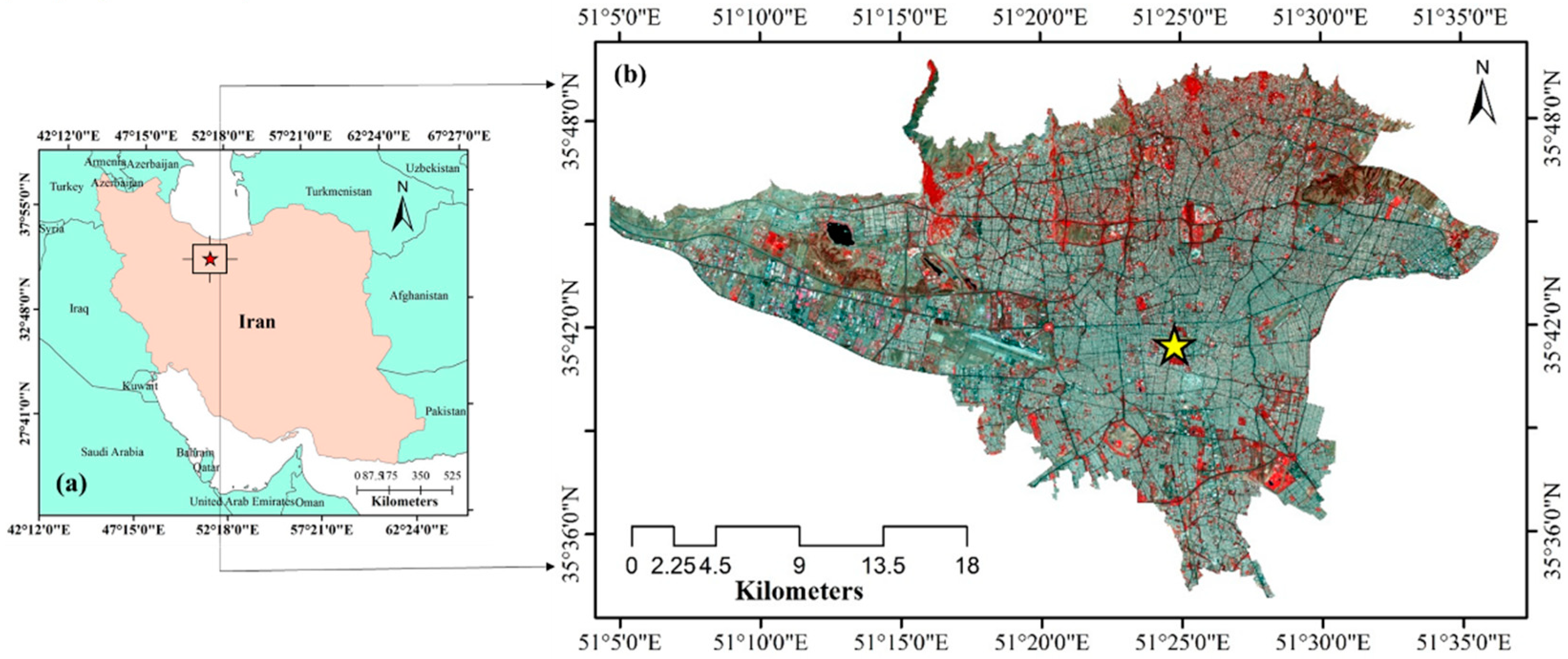
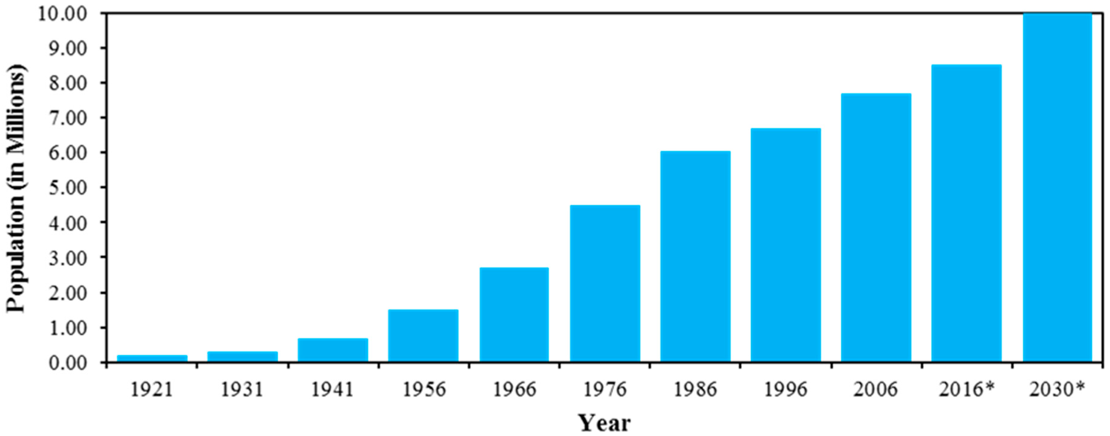
2.1. Study Area: Tehran, Iran
2.2. Satellite Images
2.3. LU/LC Retrieval
2.4. Retrieval of LST
2.5. NDVI Computation
2.6. NDBI Computation
2.7. Urban–Rural Gradient
2.8. Statistical Analysis
3. Results
3.1. Accuracy Assessment Report of LU/LC Classification
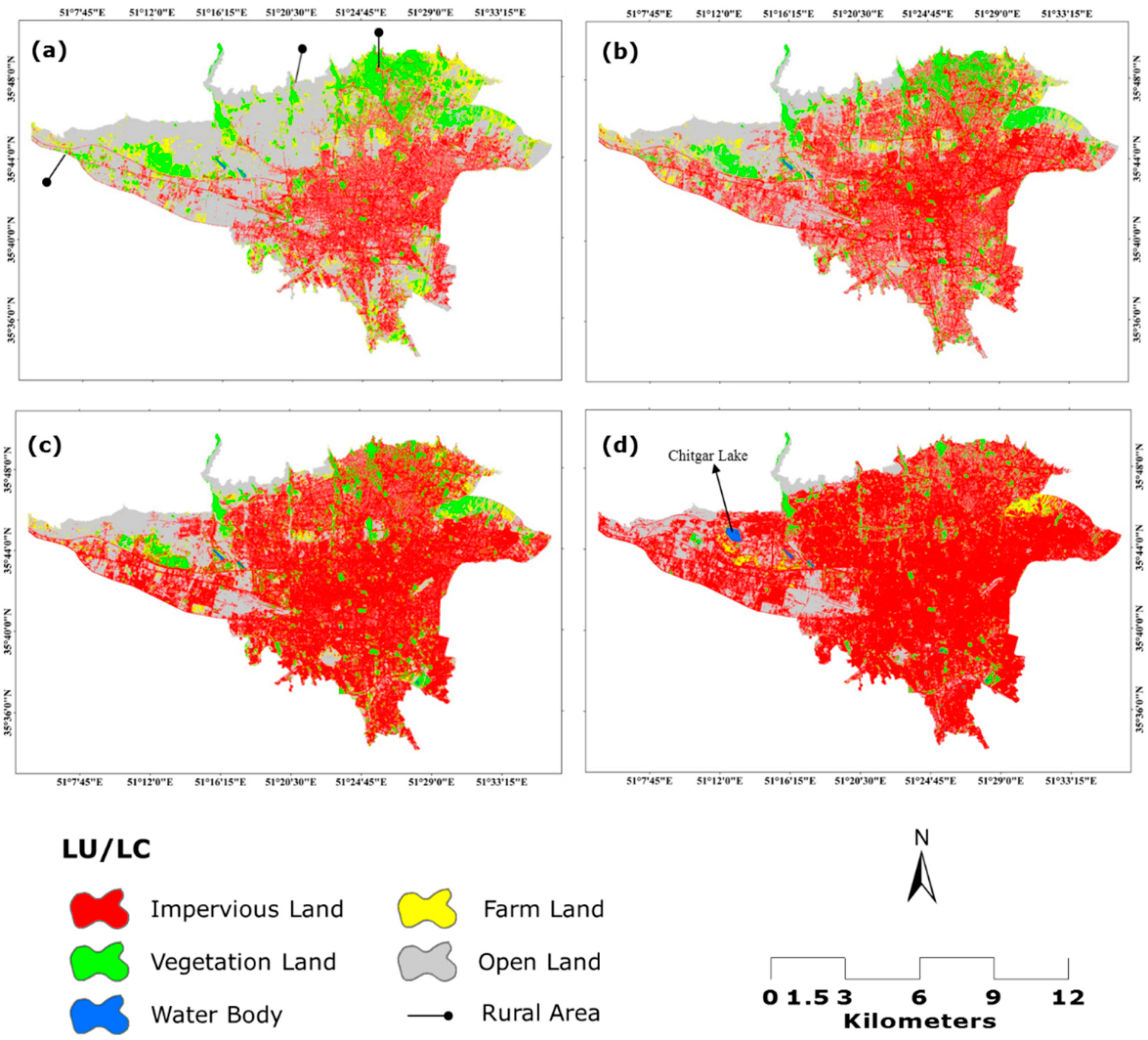
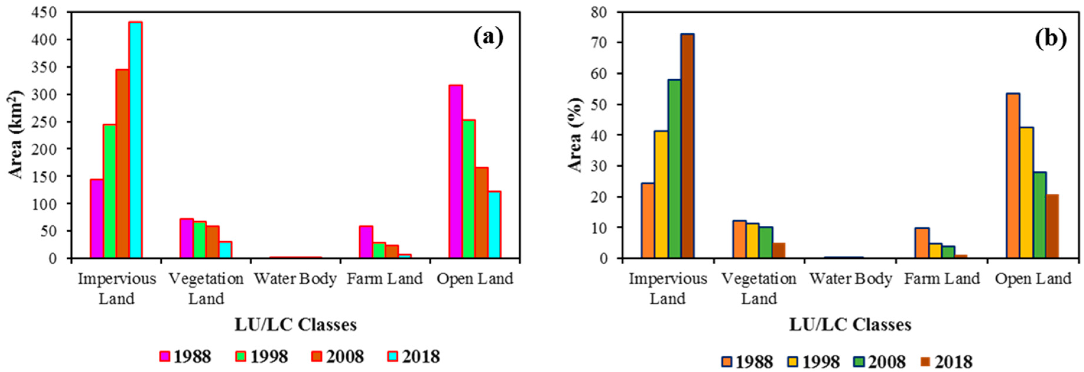
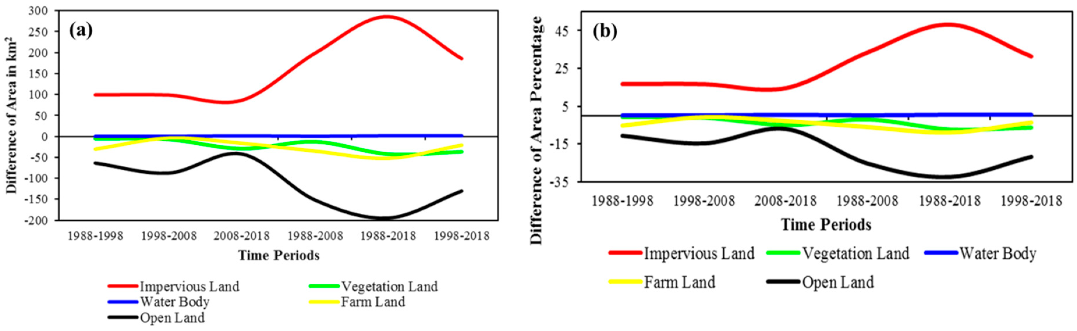
3.2. Spatiotemporal Pattern of LU/LC Dynamics
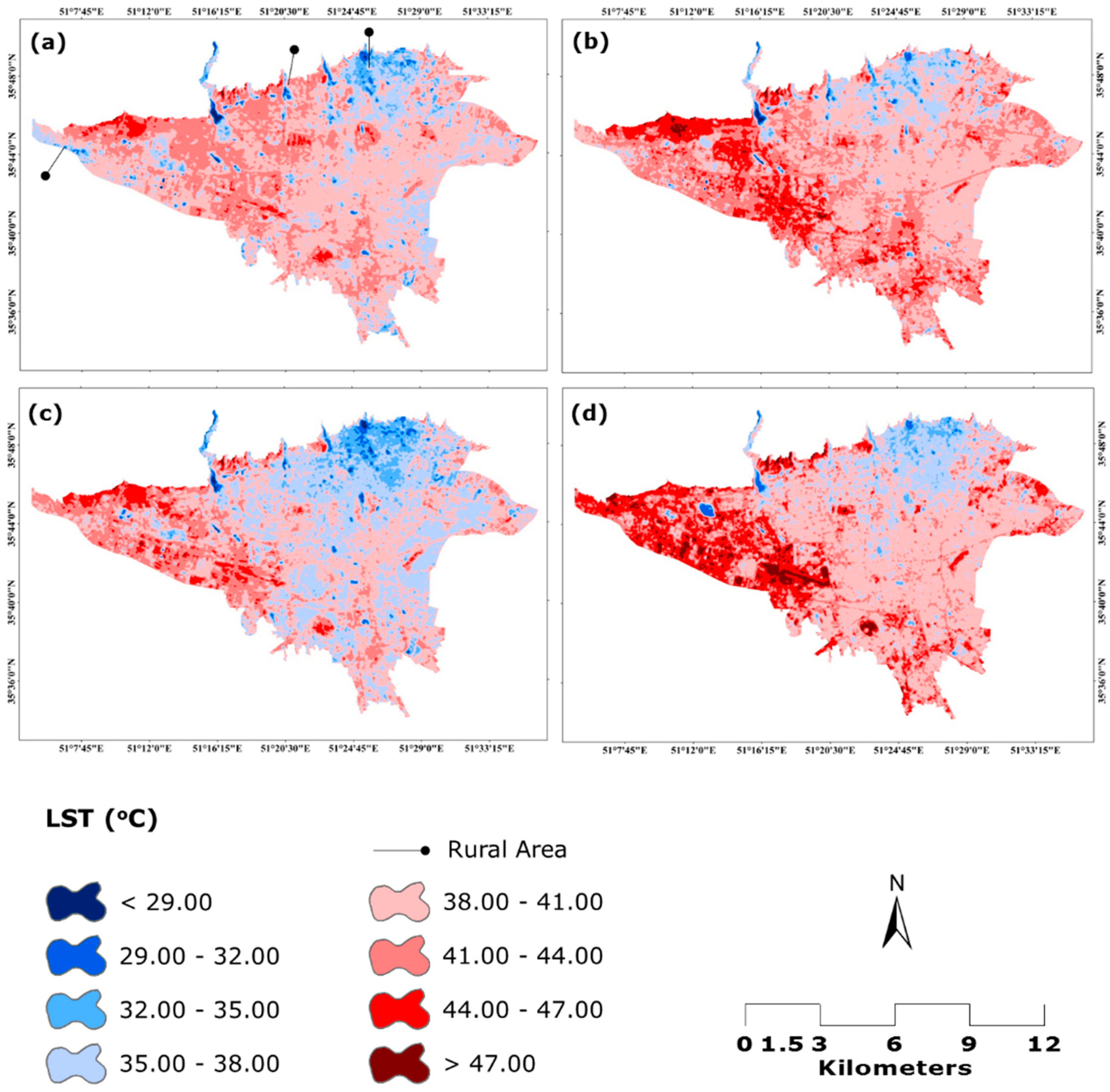
3.3. Spatiotemporal Pattern of LST Dynamics and Creation of SUHI Phenomena
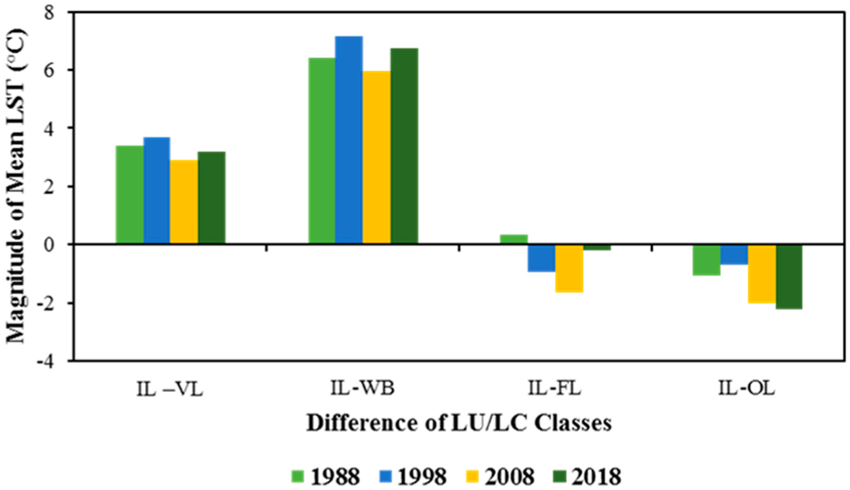
3.4. LU/LC Effects on LST
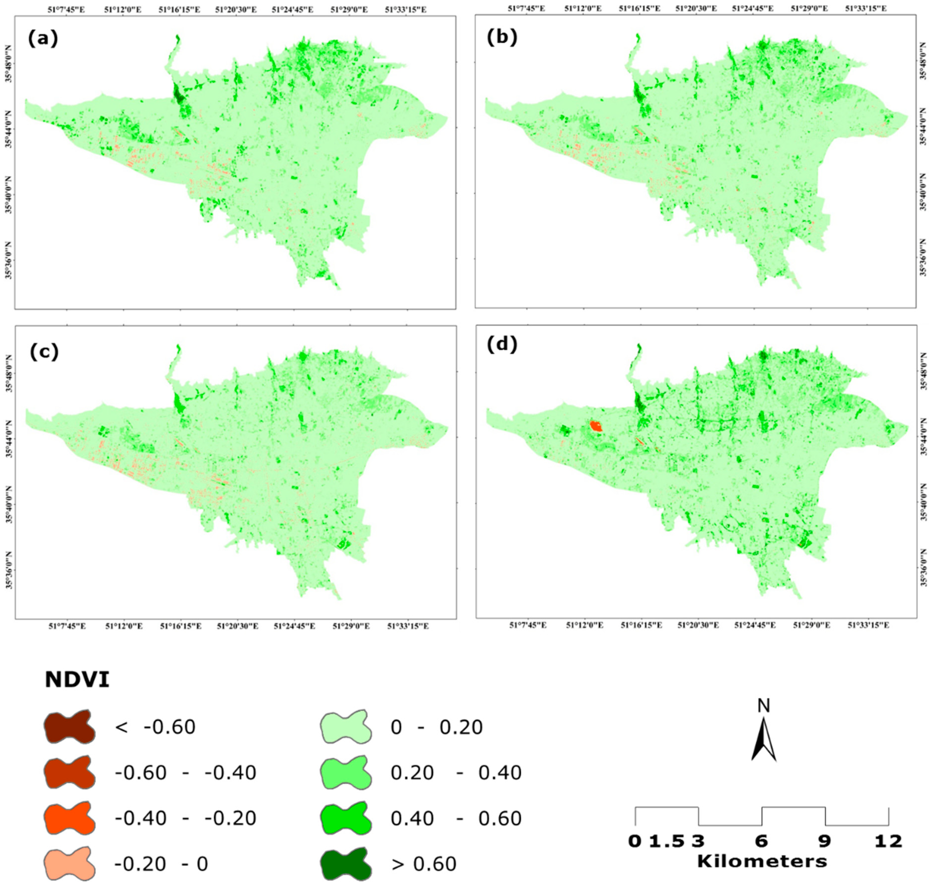
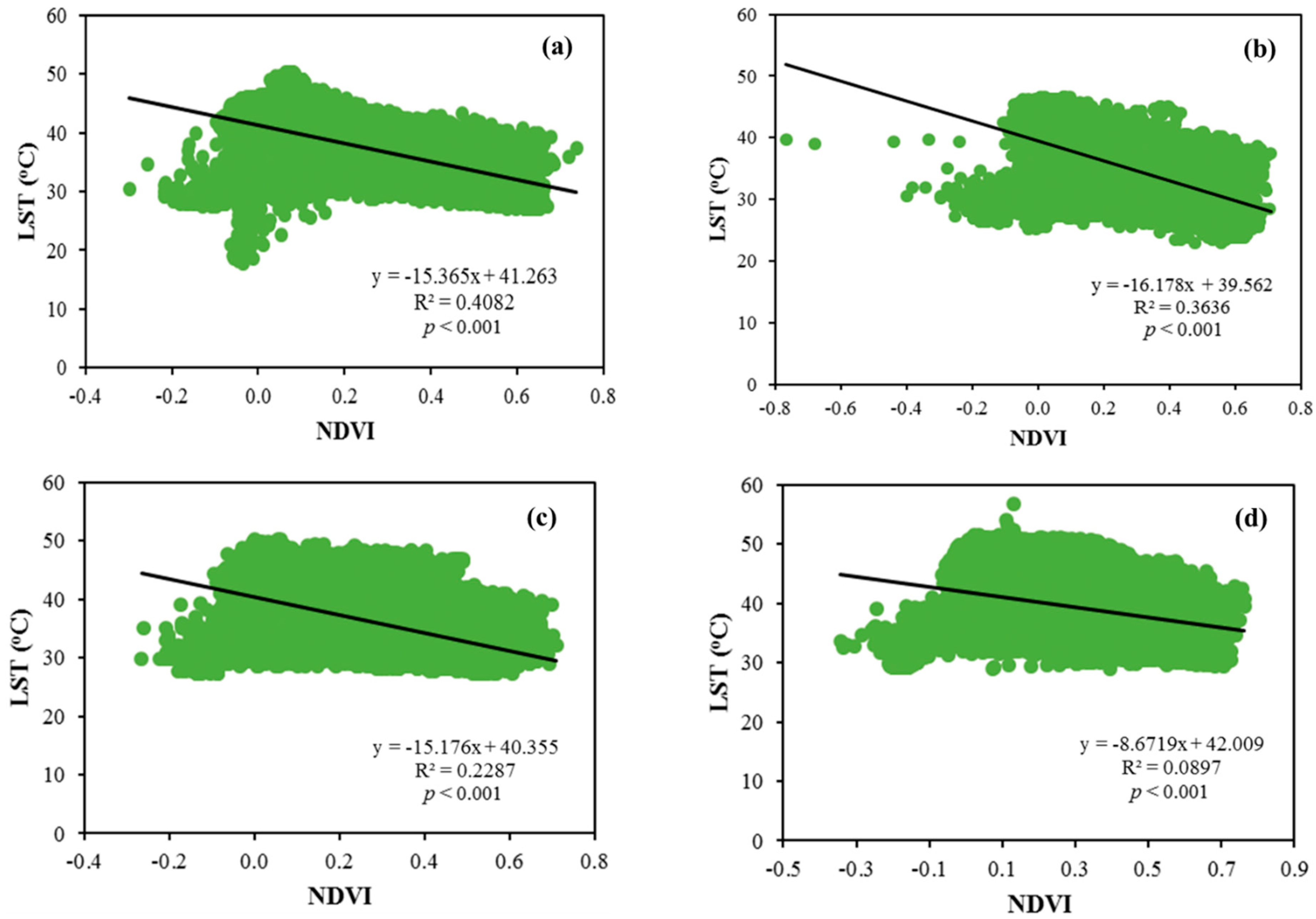
3.5. Spatiotemporal Pattern of NDVI Dynamics and Its Relationship with LST
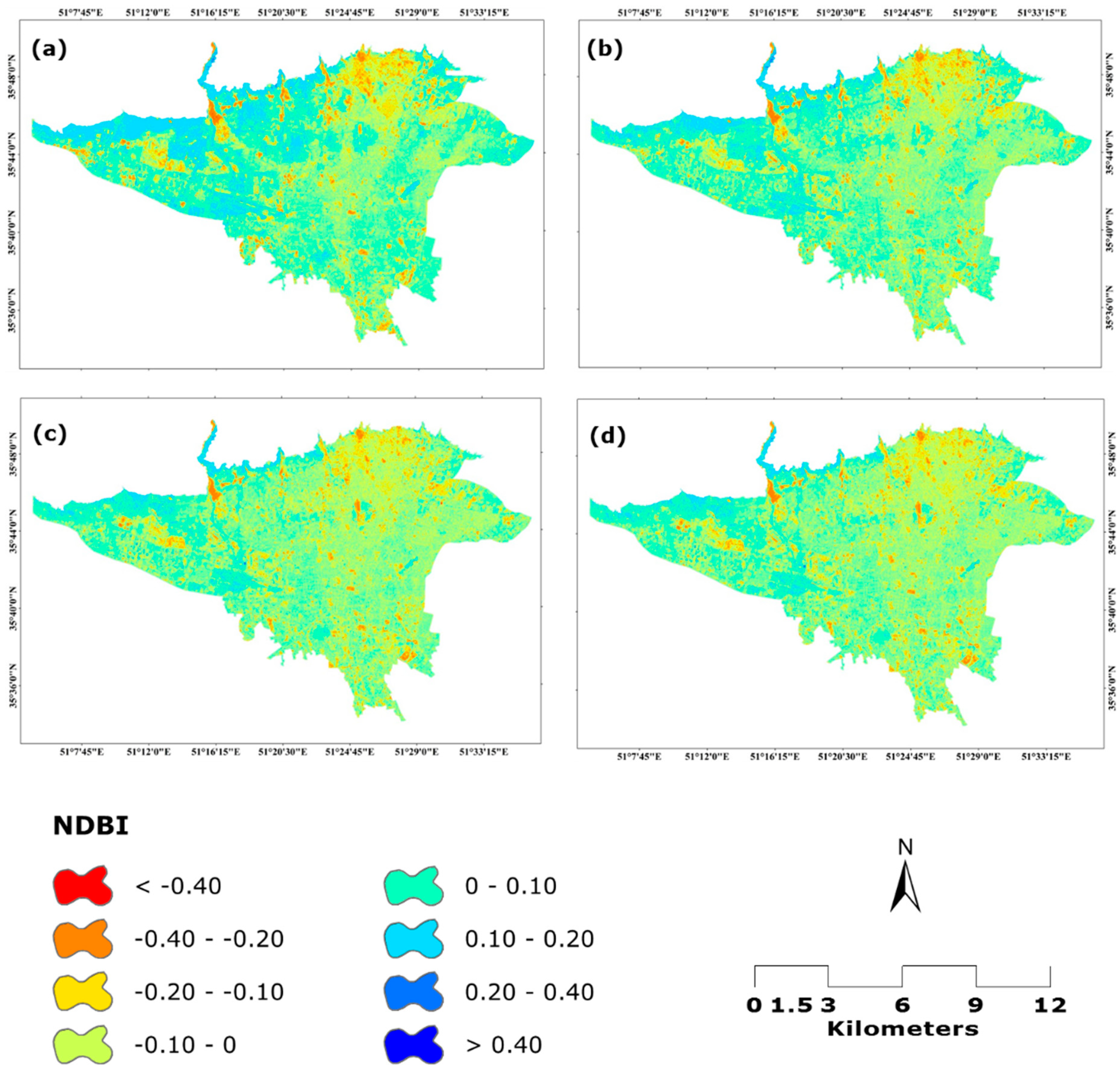
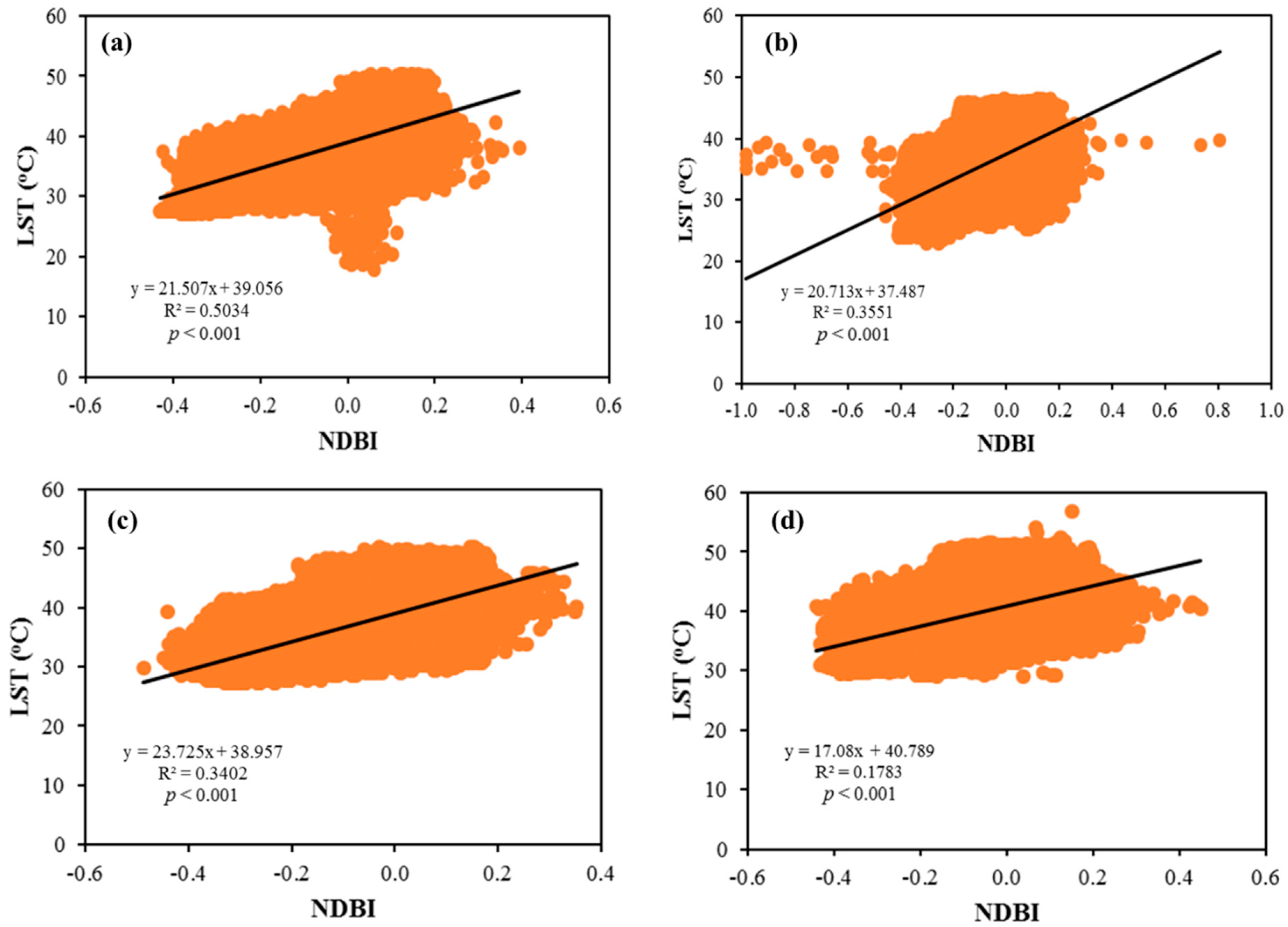
3.6. Spatiotemporal Pattern of NDBI Dynamics and Its Relationship with LST
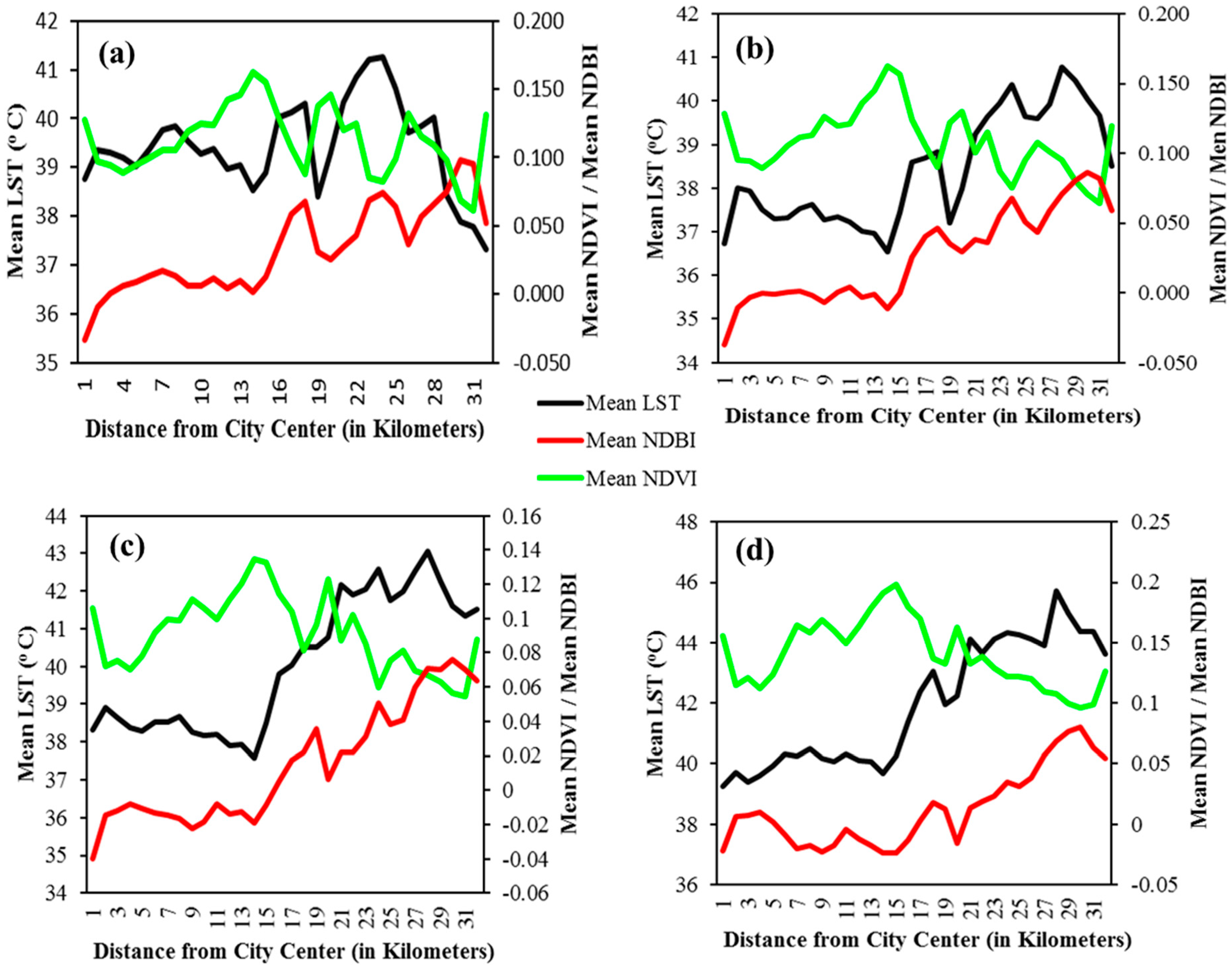
3.7. Analysis of Pattern of Urban–Rural Gradient
4. Discussion
4.1. Urbanization: An Alteration of LU/LC and Its Intensification on LST
4.2. SUHI Phenomena and Sustainable Planning
4.3. Implication of Urban Sustainability
4.4. Limitation and Future Scope of the Study
5. Conclusions
Author Contributions
Funding
Acknowledgments
Conflicts of Interest
References
- The World’s Cities in 2016. T. W. C. in 2016—D. B. (ST/ESA/S.A.), Population Deprtment, Department of Economic and Social Affairs, United Nations. 2016. Available online: http://www.un.org/en/development/desa/population/publications/pdf/urbanization/the_worlds_cities_in_2016_data_booklet.pdf (accessed on 28 August 2018).
- Wang, R.; Derdouri, A.; Murayama, Y. Spatiotemporal simulation of future land use/cover change scenarios in the Tokyo metropolitan area. Sustainability 2018, 10, 2056. [Google Scholar] [CrossRef]
- Singh, P.; Kikon, N.; Verma, P. Impact of land use change and urbanization on urban heat island in Lucknow city, Central India: A remote sensing based estimate. Sustain. Cities Soc. 2017, 32, 100–114. [Google Scholar] [CrossRef]
- Ranagalage, M.; Estoque, R.C.; Murayama, Y. An urban heat island study of the Colombo metropolitan area, Sri Lanka, based on Landsat data (1997–2017). ISPRS Int. J. Geo-Inf. 2017, 6, 189. [Google Scholar] [CrossRef]
- Ranagalage, M.; Estoque, R.C.; Handayani, H.H.; Zhang, X.; Morimoto, T.; Tadono, T.; Murayama, Y. Relation between urban volume and land surface temperature: A comparative study of planned and traditional cities in Japan. Sustainability 2018, 10, 2366. [Google Scholar] [CrossRef]
- Weng, Q.; Lu, D.; Schubring, J. Estimation of land surface temperature-vegetation abundance relationship for urban heat island studies. Remote Sens. Environ. 2004, 89, 467–483. [Google Scholar] [CrossRef]
- Sharma, R.; Chakraborty, A.; Joshi, P.K. Geospatial quantification and analysis of environmental changes in urbanizing city of Kolkata (India). Environ. Monit. Assess. 2015, 187, 4206. [Google Scholar] [CrossRef] [PubMed]
- Estoque, R.C.; Murayama, Y.; Myint, S.W. Effects of landscape composition and pattern on land surface temperature: An urban heat island study in the megacities of Southeast Asia. Sci. Total Environ. 2017, 577, 349–359. [Google Scholar] [CrossRef] [PubMed]
- Yin, J.; Yin, Z.; Zhong, H.; Xu, S.; Hu, X.; Wang, J.; Wu, J. Monitoring urban expansion and land use/land cover changes of Shanghai metropolitan area during the transitional economy (1979–2009) in China. Environ. Monit. Assess. 2011, 177, 609–621. [Google Scholar] [CrossRef] [PubMed]
- Bokaie, M.; Zarkesh, M.K.; Arasteh, P.D.; Hosseini, A. Assessment of urban heat island based on the relationship between land surface temperature and land use/land cover in Tehran. Sustain. Cities Soc. 2016, 23, 94–104. [Google Scholar] [CrossRef]
- Mirzaei, P.A. Recent challenges in modeling of urban heat island. Sustain. Cities Soc. 2015, 19, 200–206. [Google Scholar] [CrossRef]
- Babazadeh, M.; Kumar, P. Estimation of the urban heat island in local climate change and vulnerability assessment for air quality in Delhi. Eur. Sci. J. 2015, 19, 55–65. [Google Scholar]
- Son, N.T.; Chen, C.F.; Chen, C.R.; Thanh, B.X.; Vuong, T.H. Assessment of urbanization and urban heat islands in Ho Chi Minh city, Vietnam using Landsat data. Sustain. Cities Soc. 2017, 30, 150–161. [Google Scholar] [CrossRef]
- Joshi, R.; Raval, H.; Pathak, M.; Prajapati, S.; Patel, A.; Singh, V.; Kalubarme, M.H. Urban heat island characterization and isotherm mapping using geo-informatics technology in Ahmedabad city, Gujarat state, India. Int. J. Geosci. 2015, 6, 274–285. [Google Scholar] [CrossRef]
- Avdan, U.; Jovanovska, G. Algorithm for automated mapping of land surface temperature using Landsat 8 tatellite data. J. Sens. 2016, 2016, 1–8. [Google Scholar] [CrossRef]
- Rosa, A.; De Oliveira, F.S.; Gomes, A.; Gleriani, J.M.; Gonçalves, W.; Moreira, G.L.; Silva, F.G.; Ricardo, E.; Branco, F.; Moura, M.M.; et al. Spatial and temporal distribution of urban heat islands. Sci. Total Environ. 2017, 605–606, 946–956. [Google Scholar]
- Li, X.; Zhou, Y.; Asrar, G.R.; Imhoff, M.; Li, X. The surface urban heat island response to urban expansion: A panel analysis for the conterminous United States. Sci. Total Environ. 2017, 605–606, 426–435. [Google Scholar] [CrossRef] [PubMed]
- Zhang, X.; Estoque, R.C.; Murayama, Y. An urban heat island study in Nanchang City, China based on land surface temperature and social-ecological variables. Sustain. Cities Soc. 2017, 32, 557–568. [Google Scholar] [CrossRef]
- Gagliano, A.; Detommaso, M.; Nocera, F.; Evola, G. A multi-criteria methodology for comparing the energy and environmental behavior of cool, green and traditional roofs. Build. Environ. 2015, 90, 71–81. [Google Scholar] [CrossRef]
- Chaudhuri, A.S.; Singh, P.; Rai, S.C. Modelling LULC change dynamics and its impact on environment and water security: Geospatial technology based assessment. Ecol. Environ. Conserv. 2018, 24, 300–306. [Google Scholar]
- Yao, R.; Wang, L.; Huang, X.; Guo, X.; Niu, Z.; Liu, H. Investigation of urbanization effects on land surface phenology in northeast China during 2001–2015. Remote Sens. 2017, 9, 66. [Google Scholar] [CrossRef]
- Dewan, A.M.; Yamaguchi, Y. Land use and land cover change in Greater Dhaka, Bangladesh: Using remote sensing to promote sustainable urbanization. Appl. Geogr. 2009, 29, 390–401. [Google Scholar] [CrossRef]
- Ramachandra, T.V.; Kumar, U. Land surface temperature with land cover dynamics: Multi-resolution, rpatio-temporal data analysis of Greater Bangalore. Int. J. Geoinform. 2009, 5, 43–53. [Google Scholar]
- Grover, A.; Singh, R.B. Analysis of urban heat island (UHI) in relation to normalized difference vegetation index (NDVI): A comparative study of Delhi and Mumbai. Environments 2015, 2, 125–138. [Google Scholar] [CrossRef]
- Deb, S.; Kant, Y.; Mitra, D. Assessment of land surface temperature and heat fl uxes over Delhi using remote sensing data. J. Environ. Manag. 2013, 148, 143–152. [Google Scholar]
- Pandey, P.; Kumar, D.; Prakash, A.; Masih, J.; Singh, M.; Kumar, S.; Jain, V.K.; Kumar, K. A study of urban heat island and its association with particulate matter during winter months over Delhi. Sci. Total Environ. 2012, 414, 494–507. [Google Scholar] [CrossRef] [PubMed]
- Ku, D.N.; Sandeep, N.; Jyothi, S.; Madhu, T. Significant changes on land use/land cover by using remote sensing and GIS analysis-review. Int. J. Eng. Sci. Comput. 2017, 7, 5433–5435. [Google Scholar]
- Gould, W.A.; Gonz, O.M.R. Land development, land use, and urban sprawl in Puerto Rico integrating remote sensing and population census data. Landsc. Urban Plan. 2007, 79, 288–297. [Google Scholar]
- Kuang, W.; Liu, Y.; Dou, Y.; Chi, W.; Chen, G. What are hot and what are not in an urban landscape: Quantifying and explaining the land surface temperature pattern in Beijing, China. Landsc. Ecol. 2015, 30, 357–373. [Google Scholar] [CrossRef]
- Zhang, Y.; Su, Z.; Li, G.; Zhuo, Y.; Xu, Z. Spatial-temporal evolution of sustainable urbanization development: A perspective of the coupling coordination development based on population, industry, and built-up land spatial agglomeration. Sustainability 2018, 10, 1766. [Google Scholar] [CrossRef]
- Rahman, M.T.; Aldosary, A.S.; Mortoja, G. Modeling future land cover changes and their effects on the land surface temperatures in the Saudi Arabian eastern coastal city of Dammam. Land 2017, 6, 36. [Google Scholar] [CrossRef]
- Rahman, M.T. Detection of land use/land cover changes and urban sprawl in Al-Khobar, Saudi Arabia: An analysis of multi-temporal remote sensing data. ISPRS Int. J. Geo-Inf. 2016, 5, 15. [Google Scholar] [CrossRef]
- Krajewski, P.; Solecka, I.; Cetera, B.M. Landscape Change Index as a Tool for Spatial Analysis. IOP Conf. Ser. Mater. Sci. Eng. 2017, 245, 072014. [Google Scholar] [CrossRef] [Green Version]
- Krajewski, P. Assessing change in a high-value landscape: Case study of the municipality of Sobotka, Poland. Pol. J. Environ. Stud. 2017, 26, 2603–2610. [Google Scholar] [CrossRef]
- Kumar, S.; Panwar, M. Urban heat island footprint mapping of Delhi using remote sensing. Int. J. Emerg. Technol. 2017, 8, 80–83. [Google Scholar]
- Agarwal, R.; Sharma, U.; Taxak, A. Remote sensing based assessment of urban heat island phenomenon in Nagpur metropolitan area. Int. J. Inf. Comput. Technol. 2014, 4, 1069–1074. [Google Scholar]
- Mukherjee, S.; Joshi, P.K.; Garg, R.D. Analysis of urban built-up areas and surface urban heat island using downscaled MODIS derived land surface temperature data. Geocarto Int. 2017, 32, 900–918. [Google Scholar] [CrossRef]
- Lee, L.; Chen, L.; Wang, X.; Zhao, J. Use of Landsat TM/ETM+ data to analyze urban heat island and its relationship with land use/cover change. In Proceedings of the 2011 International Conference on Remote Sensing, Environment and Transportation Engineering, Nanjing, China, 24–26 June2011; pp. 922–927. [Google Scholar]
- Ranagalage, M.; Estoque, R.C.; Zhang, X.; Murayama, Y. Spatial changes of urban heat island formation in the Colombo district, Sri Lanka: Implications for sustainability planning. Sustainability 2018, 10, 1367. [Google Scholar] [CrossRef]
- Pal, S.; Ziaul, S. Detection of land use and land cover change and land surface temperature in English Bazar urban centre. Egypt. J. Remote Sens. Space Sci. 2017, 20, 125–145. [Google Scholar] [CrossRef] [Green Version]
- Zhang, Y.; Odeh, I.O.A.; Han, C. Bi-temporal characterization of land surface temperature in relation to impervious surface area, NDVI and NDBI, using a sub-pixel image analysis. Int. J. Appl. Earth Obs. Geoinf. 2009, 11, 256–264. [Google Scholar] [CrossRef]
- Thapa, R.B.; Murayama, Y. Drivers of urban growth in the Kathmandu valley, Nepal: Examining the efficacy of the analytic hierarchy process. Appl. Geogr. 2010, 30, 70–83. [Google Scholar] [CrossRef]
- Estoque, R.C.; Pontius, R.G.; Murayama, Y.; Hou, H.; Thapa, R.B.; Lasco, R.D.; Villar, M.A. Simultaneous comparison and assessment of eight remotely sensed maps of Philippine forests. Int. J. Appl. Earth Obs. Geoinf. 2018, 67, 123–134. [Google Scholar] [CrossRef]
- Roshan, G.; Rousta, I.; Ramesh, M. Studying the effects of urban sprawl of metropolis on tourism-climate index oscillation: A case study of Tehran city. J. Geogr. Reg. Plan. 2009, 2, 310–321. [Google Scholar]
- Habibi, R.; Alesheikh, A.A. An assessment of spatial pattern characterization of air pollution: A case study of CO and PM2.5 in Tehran, Iran. ISPRS Int. J. Geo-Inform. 2017, 6, 270. [Google Scholar] [CrossRef]
- Hasanlou, M.; Mostofi, N. Investigating urban heat island estimation and relation between various land cover indices in Tehran city using Landsat 8 imagery. In Proceedings of the 1st International Electronic Conference on Remote Sensing, Basel, Switzerland, 22 June–5 July 2015; pp. 1–11. [Google Scholar]
- Landsat 8 (L8) Data Users Handbook; version 2; United States Geological Survey: Sioux Falls, SD, USA, 2016; Volume 8.
- Landsat 8 (L8) Level 1 (L1) Data Format Control Book (Dfcb); version 10; United States Geological Survey: Sioux Falls, SD, USA, 2018; Volume 8.
- Sexton, J.O.; Urban, D.L.; Donohue, M.J.; Song, C. Long-term land cover dynamics by multi-temporal classi fi cation across the Landsat-5 record. Remote Sens. Environ. 2013, 128, 246–258. [Google Scholar] [CrossRef]
- Ziaul, S.; Pal, S. Image based surface temperature extraction and trend detection in an urban area of West Bengal, India. J. Environ. Geogr. 2016, 9, 13–25. [Google Scholar] [CrossRef]
- Sultana, S.; Satyanarayana, A.N.V. Urban heat island intensity during winter over metropolitan cities of India using remote-sensing techniques: Impact of urbanization. Int. J. Remote Sens. 2018, 39, 6692–6730. [Google Scholar] [CrossRef]
- Ishtiaque, A.; Shrestha, M.; Chhetri, N. Rapid urban growth in the Kathmandu valley, Nepal: Monitoring land use land cover dynamics of a himalayan city with Landsat imageries. Environments 2017, 4, 72. [Google Scholar] [CrossRef]
- Gunaalan, K.; Ranagalage, M.; Gunarathna, M.H.J.P.; Kumari, M.K.N.; Vithanage, M.; Srivaratharasan, T.; Saravanan, S.; Warnasuriya, T.W.S. Application of geospatial techniques for groundwater quality and availability assessment: A case study in Jaffna Peninsula, Sri Lanka. ISPRS Int. J. Geo-Inf. 2018, 7, 20. [Google Scholar] [CrossRef]
- Ranagalage, M.; Dissanayake, D.; Murayama, Y.; Zhang, X.; Estoque, R.C.; Perera, E.; Morimoto, T. Quantifying surface urban heat island formation in the world heritage tropical mountain city of Sri Lanka. ISPRS Int. J. Geo-Inf. 2018, 7, 341. [Google Scholar] [CrossRef]
- Emam, A.; Zolfagharian, M.; Binazadeh, K.; Deilami, H.A.; Eslaminia, A.; Bayat, J. Construction of Chitgar dam’s artificial lake -social and construction of Chitgar dam’s artificial lake—Social and environmental impact assessment. In Proceedings of the International Symposium on Appropriate technology to ensure proper Development, Operation and Maintenance of Dams in Developing Countries, Johannesburg, South Africa, 15–20 May 2016; pp. 91–100. [Google Scholar]
- Falahatkar, S.; Mousavi, S.M. Spatial and temporal distribution of carbon dioxide gas using GOSAT data over IRAN. Environ. Monit. Assess. 2017, 189, 1–13. [Google Scholar] [CrossRef] [PubMed]
- Li, D.; Sun, T.; Liu, M.; Yang, L.; Wang, L.; Gao, Z. Contrasting responses of urban and rural surface energy budgets to heat waves explain synergies between urban heat islands and heat waves. Environ. Res. Lett. 2015, 10, 1–10. [Google Scholar] [CrossRef]
- Estoque, R.C.; Murayama, Y. Monitoring surface urban heat island formation in a tropical mountain city using Landsat data (1987–2015). ISPRS J. Photogramm. Remote Sens. 2017, 133, 18–29. [Google Scholar] [CrossRef]
- Padmanaban, R.; Bhowmik, A.K.; Cabral, P.; Zamyatin, A.; Almegdadi, O.; Wang, S. Modelling urban sprawl using remotely sensed data: A case study of Chennai city, Tamilnadu. Entropy 2017, 19, 163. [Google Scholar] [CrossRef]
- Nigussie, T.A.; Altunkaynak, A.; Asce, A.M. Modeling urbanization of Istanbul under different scenarios using SLEUTH urban growth model. J. Urban Plan. Dev. 2016, 143, 1–13. [Google Scholar] [CrossRef]
- Fenta, A.A.; Yasuda, H.; Haregeweyn, N.; Belay, S.; Hadush, Z.; Gebremedhin, M.A. The dynamics of urban expansion and land use/land cover changes using remote sensing and spatial metrics: The case of Mekelle City of northern Ethiopia changes using remote sensing and spatial metrics: The case of Mekelle City of northern Ethiopia. Int. J. Remote Sens. 2017, 38, 4107–4129. [Google Scholar] [CrossRef]
- García-Ayllón, S. Rapid development as a factor of imbalance in urban growth of cities in Latin America: A perspective based on territorial indicators. Habitat Int. 2016, 58, 127–142. [Google Scholar] [CrossRef]
- Ogashawara, I.; da Silva Brum Bastos, V. A Quantitative Approach for Analyzing the Relationship between Urban Heat Islands and Land Cover. Remote Sens. 2012, 4, 3596–3618. [Google Scholar] [CrossRef] [Green Version]
- Garcia-Ayllon, S. Urban transformations as indicators of economic change in post-communist Eastern Europe: Territorial diagnosis through five case studies. Habitat Int. 2018, 71, 29–37. [Google Scholar] [CrossRef]
- Rimal, B.; Zhang, L.; Keshtkar, H.; Wang, N.; Lin, Y. Monitoring and modeling of spatiotemporal urban expansion and Land-Use/Land-Cover change using integrated Markov Chain Cellular Automata Model. ISPRS Int. J. Geo-Inf. 2017, 6, 288. [Google Scholar] [CrossRef]
- Li, J.; Wang, X.; Wang, X.; Ma, W.; Zhang, H. Remote sensing evaluation of urban heat island and its spatial pattern of the Shanghai metropolitan area, China. Ecol. Complex. 2009, 6, 413–420. [Google Scholar] [CrossRef]
- Xu, R.; Zhang, H.; Lin, H. Annual dynamics of impervious surfaces at city level of Pearl River Delta metropolitan. Int. J. Remote Sens. 2018, 39, 3537–3555. [Google Scholar] [CrossRef]
- Senanayake, I.P.; Welivitiya, W.D.D.P.; Nadeeka, P.M. Remote sensing based analysis of urban heat islands with vegetation cover in Colombo city, Sri Lanka using Landsat-7 ETM+ data. Urban Clim. 2013, 5, 19–35. [Google Scholar] [CrossRef]


| Sensor | Scene ID | Acquisition Date | Time (GMT) | Thermal Conversion Constant | |
|---|---|---|---|---|---|
| Landsat-5 TM | LT04_L1TP_164035_19880717_20170208_01_T1 | 17 July 1988 | 06:37:12 | 671.62 (Band 6) | 1284.30 (Band 6) |
| Landsat-5 TM | LT05_L1TP_164035_19980721_20171207_01_T1 | 21 July 1998 | 06:46:24 | 607.76 (Band 6) | 1260.56 (Band 6) |
| Landsat-5 TM | LT05_L1TP_164035_20080801_20161030_01_T1 | 1 August 2008 | 06:54:26 | 607.76 (Band 6) | 1260.56 (Band 6) |
| Landsat-8 OLI/TIRS | LC08_L1TP_164035_20180712_20180712_01_RT | 12 July 2018 | 07:07:15 | 774.8853 (Band 10) | 1321.0789 (Band 10) |
| Sl. No. | Class of LU/LC | Description LU/LC Class |
|---|---|---|
| 1 | IL | Impervious Land (Residential, commercial, industrial settlements, parking lots, and transport network) |
| 2 | VL | Vegetation Land (Forest-steppe and mixed forests) |
| 3 | WB | Water Bodies (Lakes, ponds, reservoirs, and open water) |
| 4 | FL | Farm Land (Crop fields and fallow field) |
| 5 | OL | Open Land (Abandoned land, barren land, bare land) |
| LU/LC Classes | Year | ||||
|---|---|---|---|---|---|
| 1988 | 1998 | 2008 | 2018 | ||
| User Accuracy | IL | 84.0 | 86.0 | 90.0 | 92.0 |
| VL | 86.0 | 82.0 | 88.0 | 90.0 | |
| WB | 100.0 | 98.0 | 100.0 | 100.0 | |
| FL | 84.0 | 88.0 | 88.0 | 90.0 | |
| OL | 82.0 | 88.0 | 92.0 | 92.0 | |
| Producer Accuracy | IL | 89.4 | 84.3 | 90.0 | 90.2 |
| VL | 91.5 | 91.0 | 89.8 | 91.8 | |
| WB | 98.0 | 96.1 | 96.2 | 98.0 | |
| FL | 89.7 | 86.3 | 89.8 | 90.0 | |
| OL | 82.0 | 80.0 | 92.0 | 92.0 | |
| Overall Accuracy | 87.2 | 88.4 | 91.6 | 92.8 | |
| Kappa Coefficient | 0.841 | 0.854 | 0.895 | 0.909 | |
| LU/LC Types | 1988 | 1998 | 2008 | 2018 | ||||
|---|---|---|---|---|---|---|---|---|
| km2 | % | km2 | % | km2 | % | km2 | % | |
| IL | 144.72 | 24.42 | 244.50 | 41.26 | 343.83 | 58.02 | 430.77 | 72.69 |
| VL | 72.19 | 12.18 | 66.80 | 11.27 | 59.47 | 10.04 | 30.14 | 5.09 |
| WB | 0.41 | 0.07 | 0.51 | 0.09 | 0.60 | 0.10 | 2.21 | 0.37 |
| FL | 58.93 | 9.94 | 28.28 | 4.77 | 23.76 | 4.01 | 6.99 | 1.18 |
| OL | 316.38 | 53.39 | 252.55 | 42.61 | 164.98 | 27.84 | 122.54 | 20.68 |
| Total | 592.64 | 100.00 | 592.64 | 100.00 | 592.64 | 100.00 | 592.64 | 100.00 |
| LU/LC Class | 1988–1998 | 1998–2008 | 2008–2018 | 1988–2008 | 1988–2018 | 1998–2018 | ||||||
|---|---|---|---|---|---|---|---|---|---|---|---|---|
| km2 | % | km2 | % | km2 | % | km2 | % | km2 | % | km2 | % | |
| IL | −99.8 | −16.8 | −99.3 | −16.8 | −86.9 | −14.7 | −199.1 | −33.6 | −286.0 | −48.3 | −186.3 | −31.4 |
| VL | 5.4 | 0.9 | 7.3 | 1.2 | 29.3 | 5.0 | 12.7 | 2.2 | 42.1 | 7.1 | 36.7 | 6.2 |
| WB | −0.1 | 0.0 | −0.1 | 0.0 | −1.6 | −0.3 | −0.2 | 0.0 | −1.8 | −0.3 | −1.7 | −0.3 |
| FL | 30.7 | 5.2 | 4.5 | 0.8 | 16.8 | 2.8 | 35.2 | 5.9 | 51.9 | 8.8 | 21.3 | 3.6 |
| OL | 63.8 | 10.8 | 87.6 | 14.8 | 42.4 | 7.2 | 151.4 | 25.6 | 193.8 | 32.7 | 130.0 | 21.9 |
| City | Date | Minimum (°C) | Maximum (°C) | Mean (°C) | Standard Deviation |
|---|---|---|---|---|---|
| Tehran | 17 July 1988 | 17.81 | 50.33 | 39.41 | 2.54 |
| 21 July 1998 | 22.94 | 46.57 | 37.62 | 2.70 | |
| 1 August 2008 | 27.25 | 50.21 | 38.80 | 2.94 | |
| 12 July 2018 | 28.92 | 56.80 | 40.65 | 3.19 | |
| The difference of Mean LST in Different Time Periods (°C) | |||||
| 1988–1998 | 1998–2008 | 2008–2018 | 1988–2008 | 1988–2018 | 1998–2018 |
| 1.79 | −1.18 | 1.85 | 0.61 | −1.24 | −3.03 |
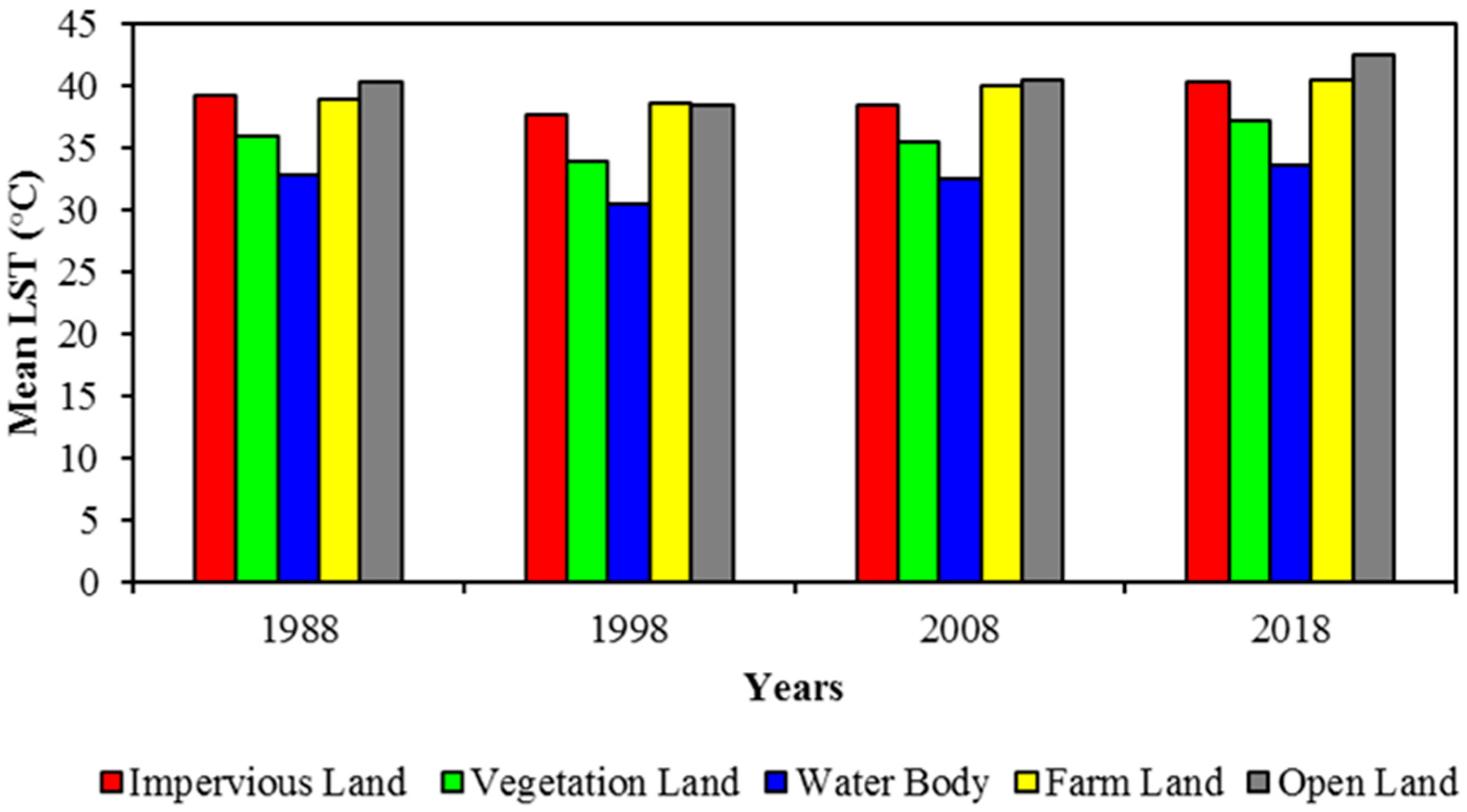
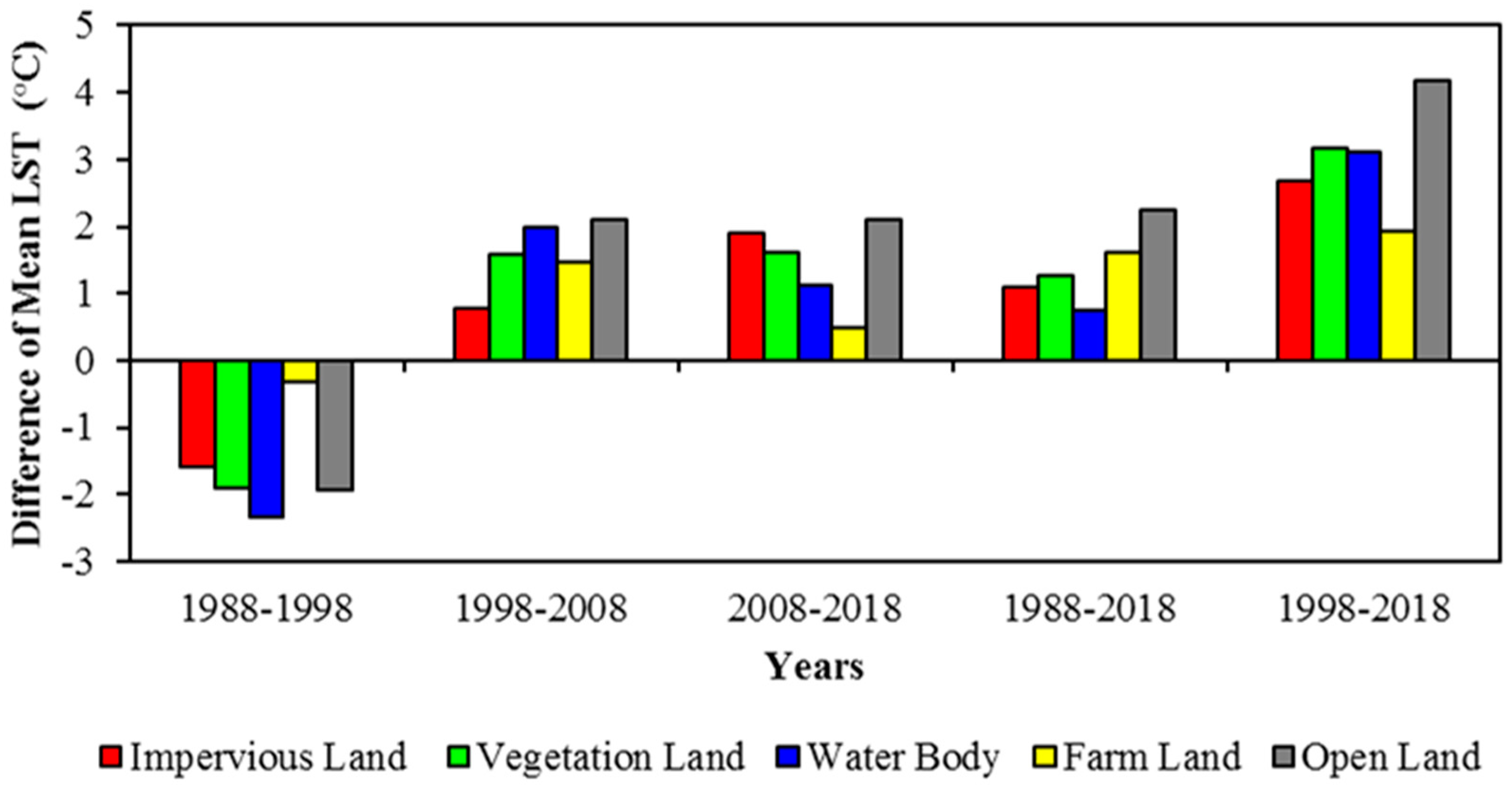
| LU/LC Class | Mean LST (°C) | The difference of Mean LST (°C) | ||||||||
|---|---|---|---|---|---|---|---|---|---|---|
| 1988 | 1998 | 2008 | 2018 | 1988–1998 | 1998–2008 | 2008–2018 | 1988–2008 | 1988–2018 | 1998–2018 | |
| IL | 39.30 | 37.70 | 38.47 | 40.38 | −1.6 | 0.77 | 1.91 | −0.83 | 1.08 | 2.68 |
| VL | 35.91 | 34.01 | 35.58 | 37.18 | −1.9 | 1.57 | 1.6 | −0.33 | 1.27 | 3.17 |
| WB | 32.87 | 30.53 | 32.52 | 33.63 | −2.34 | 1.99 | 1.11 | −0.35 | 0.76 | 3.1 |
| FL | 38.97 | 38.65 | 40.11 | 40.59 | −0.32 | 1.46 | 0.48 | 1.14 | 1.62 | 1.94 |
| OL | 40.36 | 38.41 | 40.50 | 42.60 | −1.95 | 2.09 | 2.1 | 0.14 | 2.24 | 4.19 |
| LU/LC Class (Cross Cover Comparison) | Magnitude of Mean LST (°C) | |||
|---|---|---|---|---|
| 1988 | 1998 | 2008 | 2018 | |
| IL-VL | 3.39 | 3.69 | 2.89 | 3.2 |
| IL-WB | 6.43 | 7.17 | 5.95 | 6.75 |
| IL-FL | 0.33 | −0.95 | −1.64 | −0.21 |
| IL-OL | −1.06 | −0.71 | −2.03 | −2.22 |
| City | Date | Minimum | Maximum | Mean | Standard Deviation |
|---|---|---|---|---|---|
| Tehran | 17 July 1988 | −0.30 | 0.74 | 0.12 | 0.11 |
| 21 July 1998 | −0.77 | 0.71 | 0.12 | 0.10 | |
| 1 August 2008 | −0.27 | 0.71 | 0.10 | 0.10 | |
| 12 July 2018 | −0.34 | 0.76 | 0.16 | 0.11 |
| City | Date | Minimum | Maximum | Mean | Standard Deviation |
|---|---|---|---|---|---|
| Tehran | 17 July 1988 | −0.43 | 0.39 | 0.02 | 0.08 |
| 21 July 1998 | −0.98 | 0.80 | 0.01 | 0.08 | |
| 1 August 2008 | −0.49 | 0.35 | −0.01 | 0.07 | |
| 12 July 2018 | −0.44 | 0.45 | −0.01 | 0.08 |
© 2018 by the authors. Licensee MDPI, Basel, Switzerland. This article is an open access article distributed under the terms and conditions of the Creative Commons Attribution (CC BY) license (http://creativecommons.org/licenses/by/4.0/).
Share and Cite
Rousta, I.; Sarif, M.O.; Gupta, R.D.; Olafsson, H.; Ranagalage, M.; Murayama, Y.; Zhang, H.; Mushore, T.D. Spatiotemporal Analysis of Land Use/Land Cover and Its Effects on Surface Urban Heat Island Using Landsat Data: A Case Study of Metropolitan City Tehran (1988–2018). Sustainability 2018, 10, 4433. https://0-doi-org.brum.beds.ac.uk/10.3390/su10124433
Rousta I, Sarif MO, Gupta RD, Olafsson H, Ranagalage M, Murayama Y, Zhang H, Mushore TD. Spatiotemporal Analysis of Land Use/Land Cover and Its Effects on Surface Urban Heat Island Using Landsat Data: A Case Study of Metropolitan City Tehran (1988–2018). Sustainability. 2018; 10(12):4433. https://0-doi-org.brum.beds.ac.uk/10.3390/su10124433
Chicago/Turabian StyleRousta, Iman, Md Omar Sarif, Rajan Dev Gupta, Haraldur Olafsson, Manjula Ranagalage, Yuji Murayama, Hao Zhang, and Terence Darlington Mushore. 2018. "Spatiotemporal Analysis of Land Use/Land Cover and Its Effects on Surface Urban Heat Island Using Landsat Data: A Case Study of Metropolitan City Tehran (1988–2018)" Sustainability 10, no. 12: 4433. https://0-doi-org.brum.beds.ac.uk/10.3390/su10124433