Optimal Maintenance Decision Method for Urban Gas Pipelines Based on as Low as Reasonably Practicable Principle

Abstract

In the transportation process of urban gas pipelines, there are various uncontrollable risks and uncertainties possibly leading to the failure of gas pipelines and thereby serious consequences, such as city gas shutdown, nearby casualties, and environmental pollution. To avoid these hazards, numerous studies have been performed in identifying and evaluating the occurrence of risks and uncertainties to pipelines. However, discussions on risk reduction and other maintenance work are scarce; therefore, a scientific method to guide decision making is non-existent, thereby resulting in excessive investment in maintenance and reduced maintenance cost of other infrastructures. Therefore, the as low as reasonably practicable (ALARP) principle combined with optimization theory is used to discuss pipeline maintenance decision-making methods in unacceptable regions and ALARP regions. This paper focuses on the analysis of pipeline risk reduction in the ALARP region and proposes three optimization decision models. The case study shows that maintenance decision making should consider the comprehensive impact of maintenance cost to reduce risk and loss cost caused by pipeline failure, and that the further cost–benefit analysis of measures should be performed. The proposed pipeline maintenance decision-making method is an economical method for pipeline operators to make risk decisions under the premise of pipeline safety, which can improve the effectiveness of the use of maintenance resources.

1. Introduction

Alongside urban development, urban infrastructures have to be continuously upgraded to improve the living environment of urban residents and promote economic growth. Therefore, high-speed railways, airports, bridges, tunnels, subways, gas pipelines, etc. are constructed vigorously [1,2,3]. Although these infrastructures provide convenience to residents, many uncertainties and risks are involved in the use process, such as casualties caused by derailment of rail transit [4], trapped vehicles and personnel caused by tunnel collapse [5], and water resources wastage caused by fracture of water supply pipeline [6]. Therefore, to ensure the safe operation of infrastructures throughout their life cycles and avoid the potential hazards caused by these uncertain factors to residents, the risk assessment has been proposed to identify the probability of accidents and losses [7]. Risk assessment can quantify the possibility of impacts and losses on people’s lives, properties, and other aspects before or after the occurrence of a dangerous event [8]. Afterwards, urban infrastructure operators can make decisions to reduce risk and ensure the safe operation of infrastructures. Currently, operators of urban rail transit [9], highway tunnels, bridges [10], and other infrastructure use risk-based maintenance decisions. Based on the identification of risk factors, this method can propose targeted maintenance methods, and subsequently improve the effectiveness and economy of maintenance funds.

In practice, the urban gas pipeline may be subject to a variety of comprehensive and complex risks and uncertainties, such as third-party damages, corrosion, incorrect operation of pipeline equipment operators, and manufacturing defects [11]. Moreover, the pipeline has penetrated every corner of the city, such as living areas, business circles, industrial areas, and transportation medium, where the gas is toxic, flammable, and explosive. Hence, once an accident occurs, it may cause serious consequences such as city gas shutdown, nearby casualties, and environmental pollution. In addition, owing to the increasing demand for natural gas, pipeline accidents affect the supply sustainability of energy significantly [12]. In order to avoid risk uncertainty, it is necessary to implement risk analysis on critical infrastructure. The risk analysis methods for critical infrastructure have been developed by scholars and proven to improve safety and reliability of gas pipelines [13,14]. The process is identifying the risk factors that affect the operation of pipelines and the possible consequences of pipeline failures through risk assessment, determining the high-risk pipeline section [15], and determining the risk acceptability of pipelines based on the acceptable risk level established by the government. Subsequently, operators can make decisions to consider what measures should be taken to reduce risks. However, because the urban gas pipeline system is tremendous and the environment of each pipeline section is different, the maintenance work cannot be comprehensive. Nevertheless, many operators have misunderstood the risk, and hope to reduce the risk to an extremely low level, thus resulting in the excessive use of maintenance funds for pipeline maintenance. Because the cost of pipeline maintenance belongs to the cost of urban infrastructure maintenance, if high expenditures on pipeline maintenance are wasted, the maintenance budget for other infrastructures will be reduced. Therefore, owing to the complex situation of urban gas pipelines, operators require a more scientific decision-making method to guide the allocation of maintenance funds.

In risk management, many decision-making methods exist, such as the decision tree method [16], expected value method [17], and utility function method [18]. However, these methods are dominated by the subjective preference factors of decision makers; therefore, an objective decision result cannot be obtained. In contrast, the as low as reasonably practicable (ALARP) principle proposed by HSE in Britain can obtain the objective decision-making results, which can effectively reduce risks and improve the effectiveness of maintenance funds because it is less affected by subjective factors [19,20]. Hence, this principle is often used in the operation of infrastructures with high safety requirements to make risk decisions, such as dams [21], hazardous process industries [22], railways [23], and steep urban slopes [24]. However, studies regarding the decision-making method of urban gas pipeline maintenance based on the ALARP principle are scarce. Because of insufficient failure information regarding domestic pipelines, it is difficult for cities to support a quantitative risk assessment. Therefore, the purpose of this study is to provide a quantitative maintenance decision-making method for countries with insufficient statistics of pipeline failure information to guide the formulation of risk reduction schemes, improve the safety of pipelines, and ensure a sustainable supply of natural gas. Specifically, using a city in China as an example, this study uses the idea of the ALARP principle and discusses the maintenance decision-making methods in an unacceptable region and the ALARP region, separately, based on the fuzzy fault tree quantitative risk assessment method.

The remainder of this paper is structured as follows: Section 2 discusses the quantitative risk assessment method of urban gas pipeline and the maintenance decision-making idea based on the ALARP principle. Section 3 investigates the reasonable budget of pipeline maintenance decision making in an unacceptable risk region. Section 4 focuses on the risk optimal decision-making problem in the ALARP region and proposes three optimization mathematical models. Section 5 compares the three models and selects the most economical maintenance decision-making model through a case. Finally, Section 6 concludes this paper.

2. Risk Management of Urban Gas Pipeline

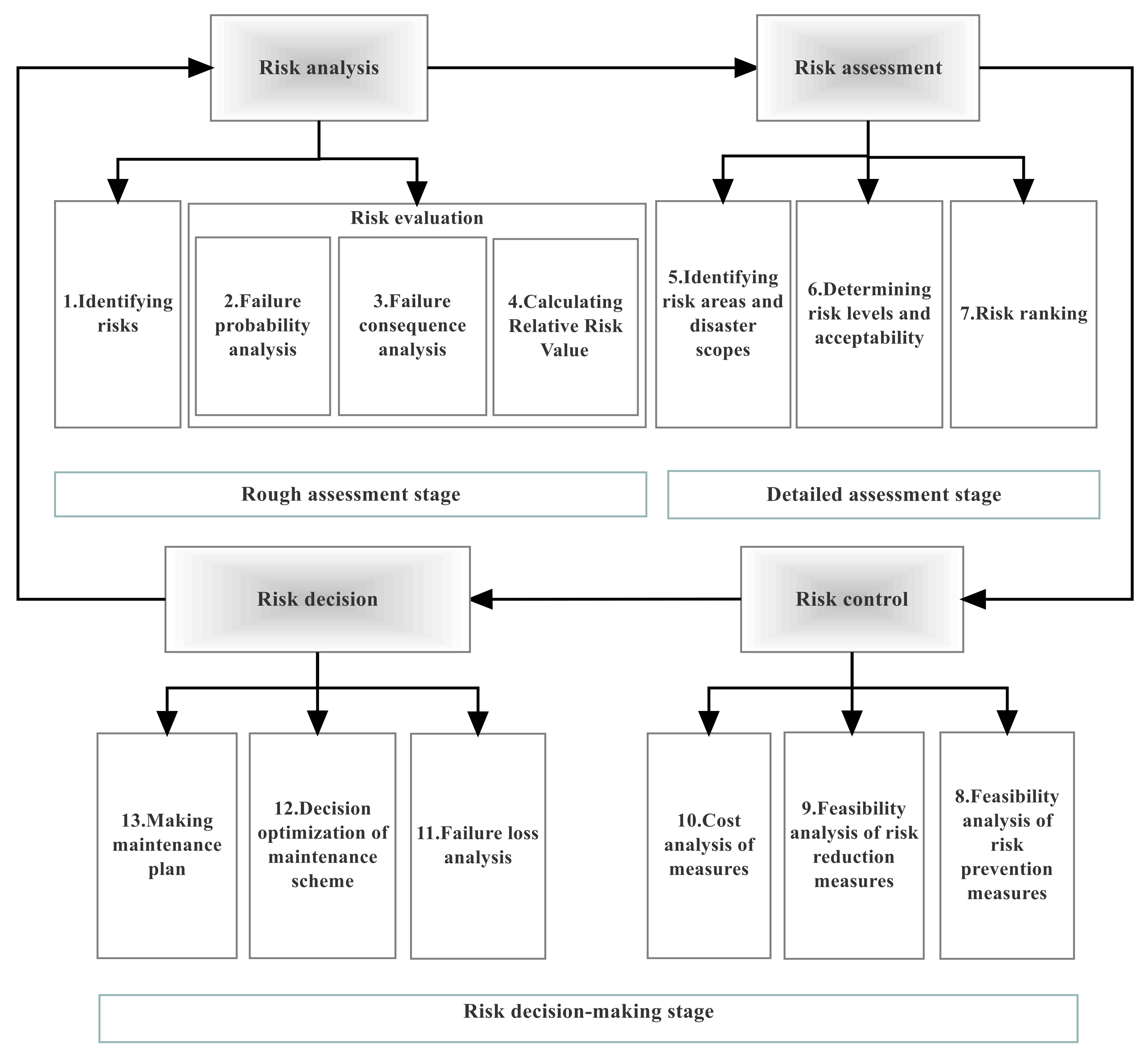
Pipeline risk management includes risk identification, risk assessment, and risk decision making. According to the identified risk factors and the corresponding assessment methods, risk assessment is performed. Finally, decision making is based on the results of risk assessment to achieve effective risk control at the lowest possible cost [25] (Figure 1).

2.1. Quantitative Risk Assessment of Pipelines

The difference between pipeline risk assessment and other equipment risk assessments is that the hazard tendency is different in the length of the whole pipeline. Owing to the diversity of various conditions along the pipeline, the risk level of each section of the whole pipeline is also different. Therefore, some indicators must be established to divide the pipe sections to obtain the accurate risk panorama. Typically, operators segment pipelines according to the size parameters, environmental changes, pressure changes, and other factors. Subsequently, the failure probability and failure consequence of each segment are evaluated separately. Finally, the risk of pipelines is integrated to obtain the total pipeline risk.

2.1.1. Failure Probability of Pipeline

Failure probability is a core content of quantitative risk assessment. It has developed gradually from the qualitative method to the quantitative method. In pipeline engineering, the calculation method of failure probability based on historical failure data is typically used, which requires a large amount of pipeline historical failure data support. The pipeline failure database of PHMSA in the USA and EGIG in Europe are mature databases that are used widely. The calculation model is as follows [26]:

$$P_i=\frac{a_i}{m}{\displaystyle \sum _{k=1}^m\frac{N_k}{L_k}}$$

(1)

where a_i is the proportion of failure factor i, which is equal to the ratio of the number of failure caused by the ith cause to the total number of faults; m = the total number of years for which the incident and mileage data are available; N_k is the number of incidents occurring on pipelines in the kth year; L_k is the corresponding length of the pipelines in the kth year, km.

In fact, owing to the late start of pipeline integrity management in many countries, the statistical failure data are insufficient to support the quantitative risk assessment of all pipelines, and only the mature failure databases of other countries can be used as data support. However, owing to the different environment and failure reasons of pipelines in other countries, it is impossible to use other countries’ failure databases directly for quantitative risk assessment. Hence, some Chinese scholars have studied the pipeline quantitative risk assessment method based on fuzzy fault tree technology and proposed an improved expert judgment method to determine the basic event probability of pipeline failure. First, the fuzzy number of an expert judgment language is obtained by fuzzifying the judgment of the pipeline basic event occurrence; subsequently, it is transformed into the fuzzy failure probability value. Subsequently the probability P_a of the basic event X_a occurrence of the fault tree is obtained. Finally, the minimum cut set is used to calculate the failure probability of the top event [27,28].

The basic events of the minimal cut set are independent of each other, and the probability P_b of the bth minimum cut set is

$$P_b={\displaystyle \prod _{X_a\in K_b}{p}_a}$$

(2)

The total failure probability of pipelines is the sum of the probability of each minimal cut set:

$$P={\displaystyle \sum _{b=1}^{\mathrm{B}}{P}_b}={\displaystyle \sum _{b=1}^{\mathrm{B}}{\displaystyle \prod _{X_a\in K_b}{p}_a}}$$

(3)

where P_a is the probability of the ath basic events, a = 1,2,…,A; K_b is the bth minimum cut set, b = 1,2,…,B.

2.1.2. Pipeline Failure Consequence

Typically, the consequences of pipeline failure are considered in three aspects: property loss, life loss, and environment loss. Property loss (PL) is the economic loss caused by pipeline failure that is recorded as c ($); life loss (LL) indicates the death toll from accidents (person) that is recorded as n (person); environmental loss (EL) can be expressed by the volume of the accident-contaminated environment medium and is recorded as v (m³). Therefore, the failure consequence C is a function of c, n, and v:

$$C=C(c,n,v)$$

(4)

Obviously, the dimensions of the three failure consequences are inconsistent; therefore, it is difficult to evaluate the loss caused by pipeline failure comprehensively. In fact, after the pipeline failure accident, for the pipeline operators, it is accompanied by economic losses such as compensation and maintenance. According to this idea, this study unifies the dimension of loss by currency quantification, which requires investigating market prices, drawing lessons from various methods of property statistics, life safety, and environmental value assessment, combined with the specific conditions of pipelines. Property loss is measured in money (c); life loss is measured by the number of casualties (n) and the corresponding compensation; environmental loss is measured by the cost of pollution control and government fines, which can be estimated according to the quantity of natural gas leakage (v) and the degree of destruction of environmental media. Ultimately, the dimensions of the three dimensions are unified as follows:

$$C(c,n,v)=S_{\mathrm{PL}}+S_{\mathrm{LL}}+S_{\mathrm{EL}}$$

(5)

where S_PL ($), S_LL ($) and S_EL ($) are monetized measurement of the loss of property, life and environment caused by pipeline failure separately.

After an accident, the loss can be divided into direct economic loss and indirect economic loss. Subsequently, total loss is

$${\mathrm{E}=\mathrm{E}}_{\mathrm{d}}+{\mathrm{E}}_{\mathrm{i}}$$

(6)

where E is the total economic loss, $; E_d is the direct economic loss, $; E_i is the indirect economic loss, $.

In general, indirect economic losses are not easy to calculate and can be estimated by direct economic losses [29]. Direct economic losses can be obtained by investigating the population, equipment, buildings, and environment medium in the region and estimating the extent of damage. Herein, the factors considered include direct property loss, life loss, and environmental loss.

• Property loss

The monetized measurement of property loss should consider the value of damaged assets and equipment, the output value of leaking media, and shutdown caused by failure [30].

• Life loss

The monetary quantification of life loss should be considered from two parts: death and injury.

For accident death, the factors to be considered in the death of a person include the following: compensation and pension according to relevant provisions; funeral expenses; arrangement expenses for family members; and government fines.

The compensation for premature death caused by pipeline accidents is typically calculated by the human capital method, that is, the loss of personal income is used to estimate the cost of premature death. According to the theory of marginal labor productivity, the value of life lost or working hours is equal to the value of personal labor during this period. The value of a person’s labor is the value of his future income converted into money, considering his age, gender, education, and other factors.

For accident injuries, the factors to be considered in the monetary quantification of personnel injuries include the following: the relevant provisions of compensation; medical expenses; nutrition expenses; rehabilitation; lost income; and government fines [31].

• Environmental loss

The impact of pipeline failure on the environment can be divided into loss of human health and loss of ecological resources.

Among them, the harm of natural gas leakage to human health in the environment is a quantitative indicator of environmental loss by monetary quantification. The monetary quantification of hazards is primarily based on the possible effects of natural gas leakage on human health (thermal radiation, noise, acute diseases, chronic carcinogenesis, etc.). This part of the loss monetary quantitative indicator primarily considers the following: compensation for the health hazards of the population; coordination costs with the population and local parties concerned; death compensation costs caused by pollution; fines of environmental protection departments; and other costs.

In addition, the primary quantitative indicators of the damage to the ecological environment caused by natural gas leakage are forest resources, soil resources, and farmland resources. When these indicators are quantified by money, they are primarily considered in the form of commodities in the market value. Simultaneously, the cost of restoring resources and the fines of environmental protection departments should be considered [32].

Therefore, the risk value ($) of pipeline is

$$R=\mathrm{P}\times (S_{\mathrm{PL}}+S_{\mathrm{LL}}+S_{\mathrm{EL}})=\mathrm{P}\times \mathrm{E}$$

(7)

2.2. Risk Acceptance Standard and ALARP Principle Decision Making

The purpose of setting risk acceptance criteria is to ensure the safety of pipelines and reasonable investment of maintenance resources, which not only guarantees the supply sustainability of petroleum energy, but also guarantees the interests of operators. Different risk acceptance criteria exhibit a common principle to seek a balance between safety and efficiency. It is impossible to evade risk completely because it will be an infinite investment. In fact, security means reducing risks to an acceptable level and achieving sufficient benefits. This idea is embodied in the ALARP principle [33].

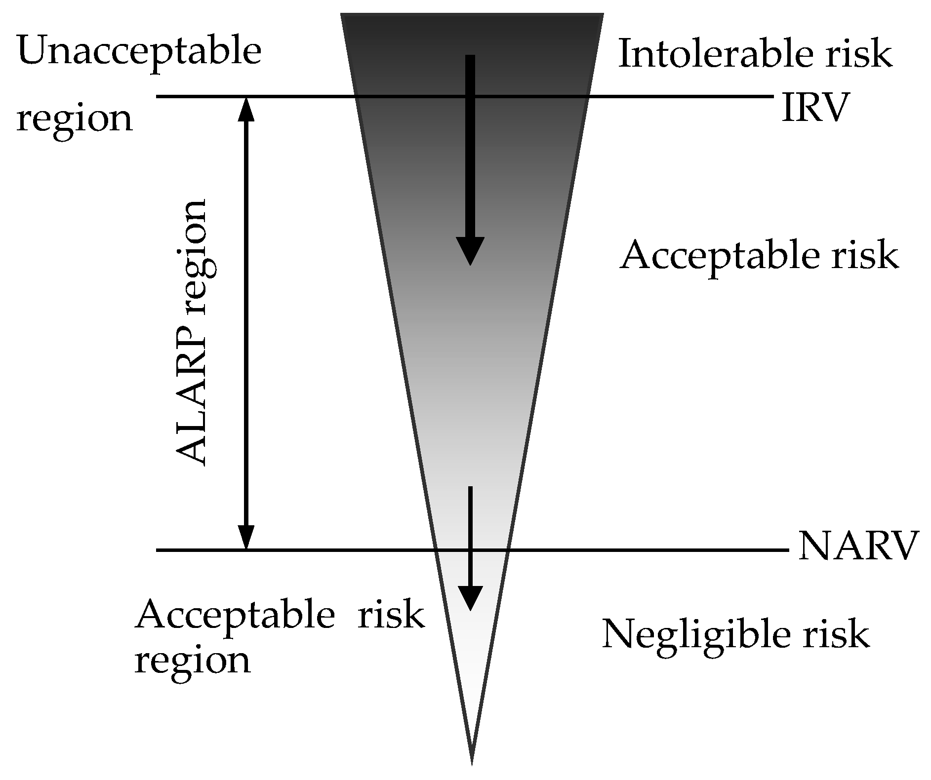
The two boundaries of ALARP (negligible value at risk (NVAR) and intolerable value (IRV)) divide risk into three regions: risk unacceptable region, risk acceptable region, and ALARP region (Figure 2). The maintenance decision-making ideas of each region are different:

• The total risk exceeds the intolerable line, and the risk is in an unacceptable region, which exhibits a greater impact on pipeline safety. Measures must be taken immediately to reduce the risk to below the intolerable line regardless of cost.
• When the total risk in the ALARP region, whether measures should be taken to reduce the risk should be weighed between the cost of taking measures and the loss that may occur without taking measures. If the cost is greater than the potential loss mitigated by the implementation of the measures, then measures are not required but rather risks should be taken. For such pipelines, the primary content of decision making is to formulate a technically feasible and economically reasonable risk reduction scheme to ensure that the risk does not exceed the intolerable line.
• When the total risk is below the negligible line, the risk is in an acceptable region. The risk is acceptable to both the public and the operators, and no measures need to be taken.

Because everything in the pipeline’s influence range exists objectively, the consequences of failure are stable in a certain time period. Therefore, this paper discusses the maintenance decision variables from the perspective of reducing pipeline failure probability.

When calculating pipeline failure probability, the occurrence probability of each basic event in the fault tree is based on the assessment of pipeline condition corresponding to the event by experts. Each basic event corresponds to many conditions, and the probability of basic events varies in all conditions. From the maintenance perspective, herein, the pipeline condition is defined to correspond to each basic event as the degree of maintenance of the measures, and the pipeline condition is classified into grades for easy measurement.

Many maintenance measures are available for an operation company, and the maintenance degree of each measure is different; furthermore, the risk value that must be reduced is different. Therefore, herein, the decision variables are the expected maintenance level of risk reduction measures. The corresponding risk reduction measures for all basic events are recorded as m_i, i = 1,2…,N; for the ith measure, the degree of risk reduction is d_j; therefore, the value space of m_i is $(m_{i_1},m_{i_2},\dots ,m_{i_{dj}})$. For a given pipe, the failure probability of the pipeline is related only to the selected maintenance scheme:

$$P=P(m_{1_1},m_{2_2},\dots ,m_{N_{dj}})$$

(8)

Based on the analysis above, pipeline maintenance decision making in an unacceptable region and ALARP region will be discussed in the following.

3. Pipeline Maintenance in Unacceptable Region

Generally, when making maintenance decisions for such pipelines in unacceptable region, because it is only necessary to consider how to reduce the risk value to below the unacceptable line and the cost need not be considered, it is often over-maintained, thus resulting in the unnecessary waste of resources. Therefore, this section provides a maintenance budget model based on cost–benefit analysis to avoid the over-maintenance of pipelines in the region.

3.1. Cost–Benefit Analysis

Cost–benefit analysis is an analysis method to evaluate the feasibility of decision making by weighing the costs and benefits, which focuses on the measurement and comparison of costs and benefits. Pipeline maintenance costs include basic costs (pipeline design, construction, and operation and management costs) and ancillary costs (safety and security measures costs). Meanwhile, the benefits of maintenance measures include direct benefits (economic benefits from completing transportation tasks) and indirect benefits (goodwill value of enterprises, etc.).

In cost–benefit measurement, because indirect benefit is not a commodity, no market price exists; therefore, it is difficult to estimate its value [34]. Hence, in cost–benefit measurement, only the direct benefits yielded by the implementation of measures are considered herein, that is, the maintenance of pipelines is simply regarded as an economic activity, and the benefits can be expressed by the reduced risk value. Hence, the advantages and disadvantages of the measures can be compared to choose the appropriate measures to reduce risks.

The cost–benefit analysis primarily considers one parameter: Return on investment (ROI). ROI is the ratio of input cost (measure cost, $/km) to benefit (risk reduction value, $), which represents the cost required to take measures to reduce the unit risk value. The larger the value, the higher is the cost.

$$\mathrm{ROI}=\frac{\mathrm{measures} \mathrm{cost}}{\mathrm{risk} \mathrm{reduction} \mathrm{value}}=\frac{C_{mi}}{\Delta R}$$

(9)

where $\Delta R=R_{k0}-{\mathrm{IRV}}_k$; R_k0 is the current risk value of the kth segment, k = 1,2, …, K; C_mi is the cost of the ith measure.

3.2. Maintenance Budget Calculation Model

According to the analysis above, operators should select ROI low measures to reduce risk. Therefore, it is necessary to rank the measures that operators can take based on cost- benefit analysis. The ROI low measures rank ahead. Operators should select a set from the front measures to the back according to the ranking, such that the measures in the set can reduce the risk value by 1. However, it is difficult to find exactly 1. Conservatively, measure addition to the set should be stopped when all measures in the set can reduce the risk value by greater than or equal to 1, and any of the measure is removed in this set, the reduced risk value will be less than 1.

The minimum cost maintenance measures for reducing the unit risk values are recorded as M₁.

$${\mathrm{M}}_1={\left\{\mathrm{Maintenance} \mathrm{measures} \mathrm{to} \mathrm{reduce} \mathrm{unit} \mathrm{risk}\right\}}_{\min }$$

$$\mathrm{S}.\mathrm{T}. \underset{i=1}{\overset{N_1}{\Delta }}{R}_{{\mathrm{M}}_{1i}}\ge 1 \mathrm{and} \underset{i=1}{\overset{N_1-1}{\Delta }}{R}_{{\mathrm{M}}_{1i}}<1$$

where i is the code of the measures in M₁, i = 1,2,...,N1; $\underset{i=1}{\overset{N}{\Delta }}{R}_{{\mathrm{M}}_{1i}}$ is defined as the risk value that can be reduced after the implementation of measures in M₁. By adding the ROI values corresponding to each measure in the set and combining the difference between the risk value and the tolerable line of the pipe segment, the minimum maintenance cost $C_{1k}$ ($/km) of the unit length pipe segment can be obtained.

$$C_{1k}=(R_{k0}-{\mathrm{IRV}}_k){\displaystyle \sum _{i=1}^{N_1}{\mathrm{ROI}}_{M_{1i}}}$$

(10)

The minimum budget C₁ ($) model for calculating the risk value of each pipe segment to reach the IRV_k can be derived in the unacceptable region:

$$C_1={\displaystyle \sum _{k=1}^K{C}_{1k}}{l}_k={\displaystyle \sum _{k=1}^K(R_{k0}-{\mathrm{IRV}}_k){\displaystyle \sum _{i=1}^{N_1}{\mathrm{ROI}}_{M_{1i}}}}{l}_k$$

(11)

where l_k is the length of the kth pipe segment.

On the contrary, according to the rank, operators should select a set record as M₂ from the measure from the behind to the front, so that measures in the set can reduce the risk value by 1. The maximum budget C₂ ($) model for calculating the risk value of each pipe segment to reach the IRV_k can be derived in the unacceptable region:

$$C_2={\displaystyle \sum _{k=1}^K{C}_{2k}}{l}_k={\displaystyle \sum _{k=1}^K(R_{k0}-{\mathrm{IRV}}_k){\displaystyle \sum _{k=1}^{N_2}{\mathrm{ROI}}_{M_{2i}}}}{l}_k$$

(12)

$$\mathrm{S}.\mathrm{T}. \underset{i=1}{\overset{N_2}{\Delta }}{R}_{{\mathrm{M}}_{2i}}\ge 1 \mathrm{and} \underset{i=1}{\overset{N_2-1}{\Delta }}{R}_{{\mathrm{M}}_{2i}}<1$$

where i is the code of the measures in M₂, i = 1,2, ..., N2.

It is reasonable to reduce the risk budget in this region by (C₁, C₂).

4. Pipeline Maintenance in ALARP Region

In this section, pipeline maintenance decision making in the ALARP region will be discussed. Considering that the urban pipeline system is huge, many risk factors affect its normal operation; therefore, maintenance funds need to be allocated more reasonably. In addition, maintenance schemes should be obtained through maintenance focus in different regions. This paper introduces the optimization theory and proposes three decision-making models for optimal maintenance based on the ALARP principle. They are: the optimal risk value model with maintenance cost limitation, the optimal maintenance cost model with risk limitation, and the improved comprehensive optimization model of loss-maintenance total cost.

4.1. Optimal Risk Value Model with Maintenance Cost Limitation

Reducing the risk in the region no longer relates to the unlimited cost in maintaining the pipeline in the unacceptable region. Generally, pipeline operators will plan a certain budget in advance, formulate pipeline maintenance strategy in this budget, select appropriate risk reduction measures, and strive to minimize pipeline risk value. Therefore, the model is based on a maintenance cycle maintenance cost budget formulated by pipeline operators as a constraint condition, and reasonable risk reduction measures are selected to obtain the lower pipeline risk.

The objective function is

$${\min }_{ }R=\min P(m_{1_1},m_{2_2},\dots ,m_{N_{dj}})\times (S_{\mathrm{PL}}+S_{\mathrm{LL}}+S_{\mathrm{EL}})$$

(13)

The constraint of the model is that the total cost of maintenance measures is no more than that of the operator’s maintenance budget B_Total:

$$\mathrm{S}.\mathrm{T}. C_m(m_{1_1},m_{2_2},\dots ,m_{N_{dj}})={\displaystyle \sum _{i=1}^N{C}_{mi}}\le B_{\mathrm{Total}}$$

where C_m is the total cost of implementing maintenance.

The advantage of this model is that it can fully utilize the maintenance budget and spend the maintenance cost most reasonably in the maintenance measures. Moreover, the effect of risk reduction in this cycle can be used to guide the maintenance budget setting in the next maintenance cycle.

4.2. Optimal Maintenance Cost Model with Risk Limitation

In addition to the maintenance scheme described in the previous section, in some desolate and uninhabited areas, operators only need to control the risk within the scope of ALARP and focus on reducing maintenance costs when formulating maintenance strategies. Based on this idea, this section proposes an optimal maintenance cost model with risk limitation; it uses risk as constraint and maintenance cost as an optimization objective. The cost is the sum of the implementation costs of all maintenance measures, and the objective function is

$$\min C_m(m_{1_1},m_{2_2},\dots ,m_{N_{dj}})=\min {\displaystyle \sum _{i=1}^N{C}_{mi}}$$

(14)

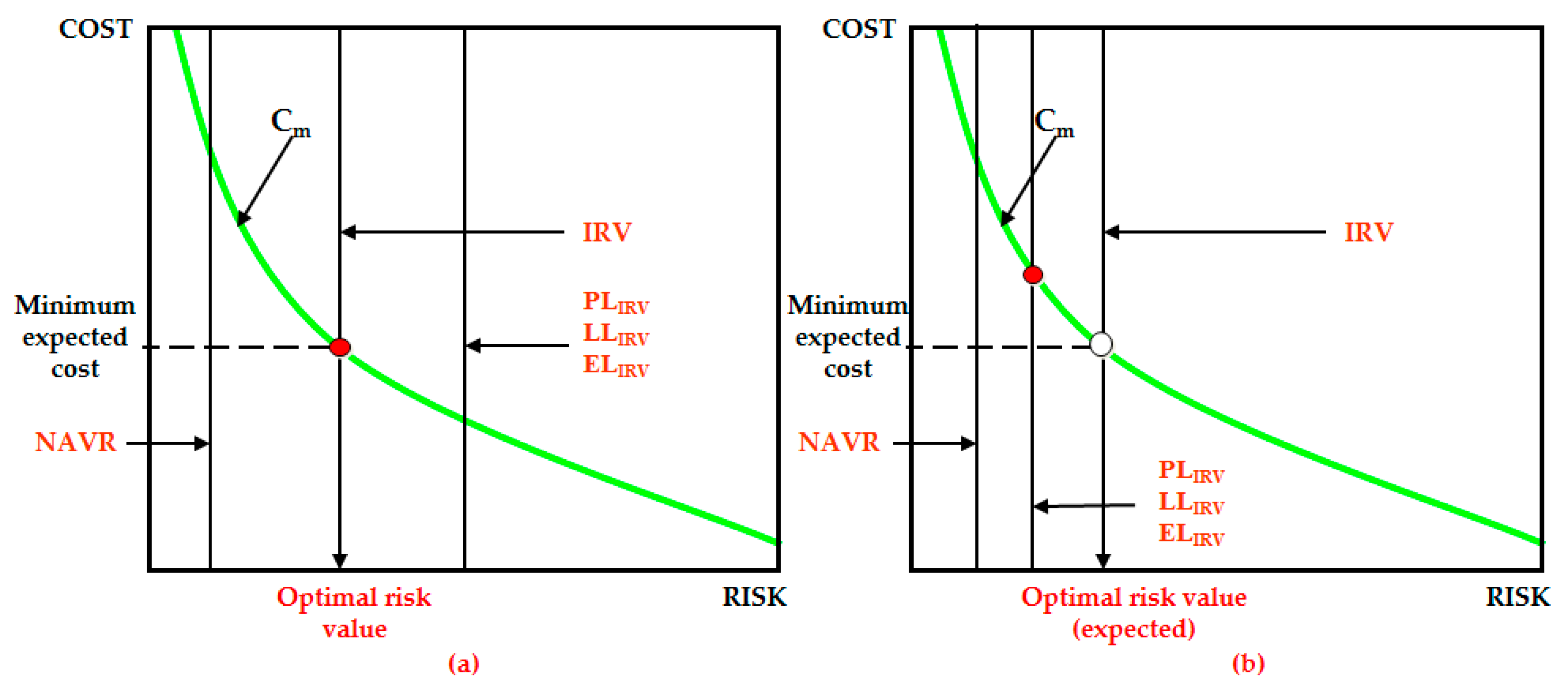
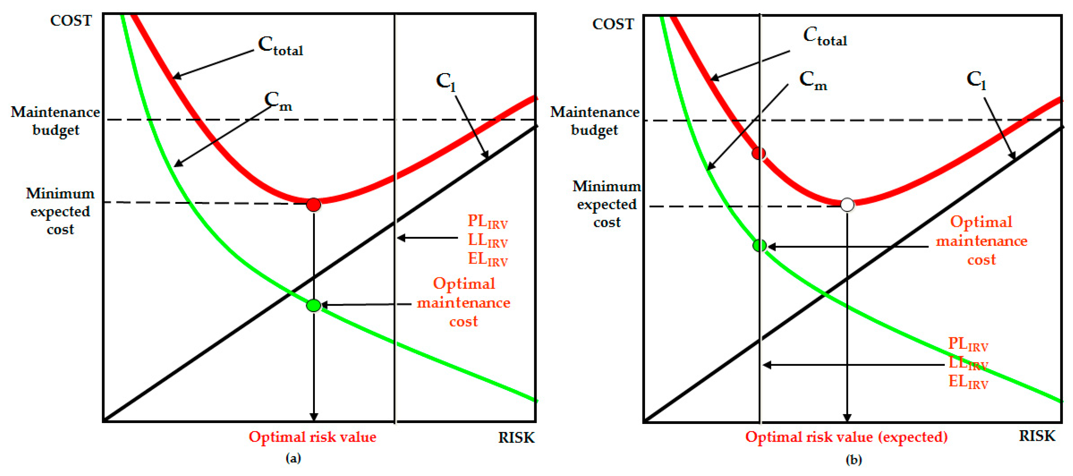
The pipeline maintenance scheme should be formulated according to the actual situation of the routing area. The protection focus in different area is different, involving population, environment and property. Once damaged, the consequences are very serious. Therefore, when maintenance decisions are formulated, the risk of damage to the protection focus should be controlled within acceptable limits. In addition to the two boundaries of ALARP, the acceptable criteria of life loss risk (LR), environmental loss risk (ER), and property loss risk (PR) are used as constraints to ensure the safety of life, environment, and property near the pipeline. The graph is used to illustrate the model (Figure 3), where the ordinate is cost and the abscissa is risk. As shown in Figure 3a, the optimal solution based on the unacceptable risk constraint satisfies the maximum allowable loss risk criteria, which is feasible. In Figure 3b, the optimal risk value does not satisfy the maximum allowable loss risk criteria; therefore, the optimal solution that satisfies the maximum allowable loss risk criteria should be chosen.

Therefore, the constraint conditions of the model are as follows:

$$\mathrm{S}.\mathrm{T}. \mathrm{NVAR}<R=P(m_{1_1},m_{2_2},\dots ,m_{N_{dj}})\times (S_{\mathrm{PL}}+S_{\mathrm{LL}}+S_{\mathrm{EL}})<\mathrm{IRV}$$

$$PR\le P{R}_{IRV}$$

$$LR\le L{R}_{IRV}$$

$$ER\le E{R}_{IRV}$$

The advantage of the model is to minimize the maintenance cost, considering the three aspects of life safety, property safety, and environmental protection.

4.3. Improved Comprehensive Optimization Model of Loss-Maintenance Total Cost

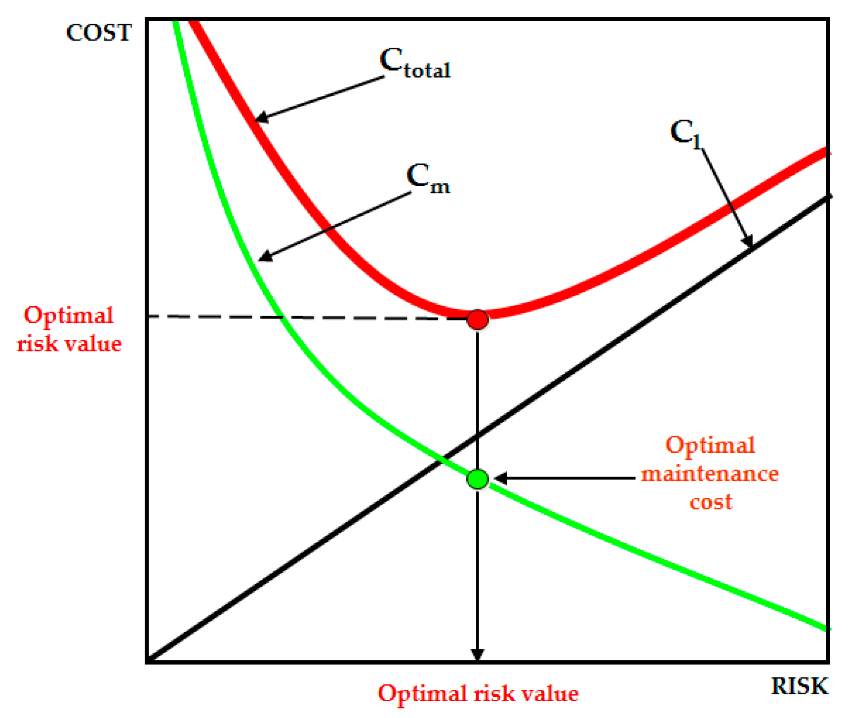
The first two models are currently widely used, and both models have their own effects on maintenance. However, they do not fully consider the benefits of operators. Risk cost is the investment of operators in risk management and control. Generally, the risk cost that operators invest in equipment risk management includes not only the cost for reducing risk, but also the loss cost that may be caused by equipment failure. That is, the maintenance cost (C_m) and possible loss (C_l) should be considered comprehensively in making maintenance decisions; subsequently, the scheme with the lowest total cost should be chosen. The comprehensive optimization model of loss–maintenance total cost was proposed by Maher in 1995 and considers the combined effects of both costs [35]. Combined with the urban gas pipeline project, the total risk cost is equal to the maintenance cost and possible loss cost of pipeline failure. Therefore, the objective function is

$$\min C_{\mathrm{total}}=C_{\mathrm{m}}+C_{\mathrm{l}}$$

(15)

The original model proposed by Maher is shown in Figure 4, where the ordinate is cost and the abscissa is risk. The total cost is superimposed by two curves of maintenance cost and failure loss cost, aiming at the lowest total risk cost. In fact, this is an ideal model, which only considers the impact of two types of costs on the total cost. It is inconsistent with the actual pipeline risk management; therefore, the optimal solution obtained is worth discussing. Next, the original model is improved by combining the ALARP principle and the factors that must be considered in the actual pipeline risk management.

Generally, the pipeline operators will generate maintenance budgets so that the total risk cost will not exceed the budget. In addition, pipeline risks should be tolerated, and life, environment, and property safety should be guaranteed.

In addition, cost–benefit analysis should be used to assess the feasibility of the measures in the ALARP region. Cost–benefit in pipeline risk decision making primarily considers the following factors: measures cost (C_m), direct benefit (I), failure probability (P), and loss of failure (C_l) of pipeline after maintenance. In conjunction with these four factors, the following mathematical models are used to represent the total benefits:

$${\mathrm{E}}_{\mathrm{T}}=f\left(\mathrm{I},C_{\mathrm{m}},C_{\mathrm{l}},\mathrm{P}\right)$$

(16)

The expected benefit of E_P is

$${\mathrm{E}}_{\mathrm{p}}=\mathrm{I}(1-\mathrm{P})+(-{\mathrm{C}}_{\mathrm{l}}\mathrm{P})=\mathrm{I}(1-\mathrm{P}(m_{1_1},m_{2_2},\dots ,m_{N_{dj}}))-{\mathrm{C}}_{\mathrm{l}}\mathrm{P}(m_{1_1},m_{2_2},\dots ,m_{N_{di}})$$

(17)

The total benefit is equal to the expected benefit minus the cost of the measure; therefore, the total benefit E_T can be calculated from the following formula:

$${\mathrm{E}}_{\mathrm{T}}={\mathrm{E}}_{\mathrm{p}}-C_m=\mathrm{I}(1-\mathrm{P}(m_{1_1},m_{2_2},\dots ,m_{N_{dj}}))-{\mathrm{C}}_{\mathrm{l}}\mathrm{P}(m_{1_1},m_{2_2},\dots ,m_{N_{di}})-C_m$$

(18)

These measures are feasible when ET > 0. Therefore, the constraints of the model are the following:

$$\mathrm{S}.\mathrm{T}. \mathrm{NVAR}<R=P(m_{1_1},m_{2_2},\dots ,m_{N_{dj}})\times (S_{\mathrm{PL}}+S_{\mathrm{LL}}+S_{\mathrm{EL}})<\mathrm{IRV}$$

$$PR\le P{R}_{IRV}$$

$$LR\le L{R}_{IRV}$$

$$ER\le E{R}_{IRV}$$

$$C_m(m_{1_1},m_{2_2},\dots ,m_{N_{dj}})={\displaystyle \sum _{i=1}^N{C}_{mi}}\le B_{\mathrm{Total}}$$

$$\mathrm{I}(1-\mathrm{P}(m_{1_1},m_{2_2},\dots ,m_{N_{dj}}))-(S_{\mathrm{PL}}+S_{\mathrm{LL}}+S_{\mathrm{EL}})\mathrm{P}(m_{1_1},m_{2_2},\dots ,m_{N_{dj}})-C_m>0$$

The improved model is shown in Figure 5. Figure 5a is the optimal solution obtained under the premise that all constraints are satisfied, which is feasible. As shown in Figure 5b, when the optimal risk value does not satisfy the maximum allowable loss risk constraint, the optimal economic solution under the maximum allowable loss risk constraint should be chosen. The model not only considers the impact of maintenance cost and loss cost on total cost, but also adds the cost–benefit analysis and maximum allowable loss risk criterion to the constraints, such that the solution can be balanced in terms of cost, benefit, life safety, environmental protection, and property safety. Thus, a new problem arises. It is necessary to find the most comprehensive and optimal model among the three models in guaranteeing benefits of operators and safety of pipelines. Therefore, a case is used to compare and analyze three models.

5. Case Analysis

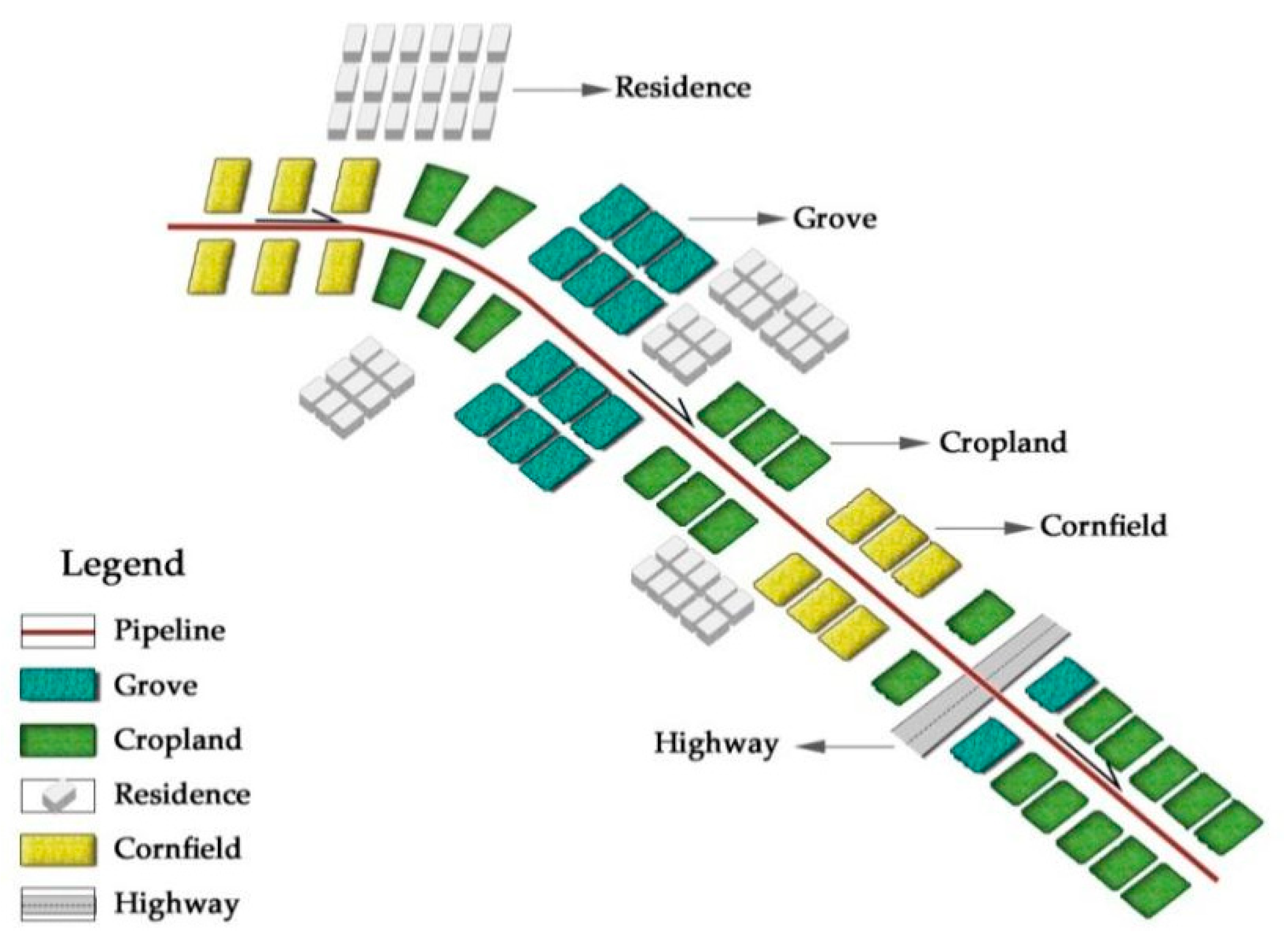
A 10-km buried gas pipeline is divided into 20 sections for risk assessment in Zhongmiao Village, Dazhou City, Sichuan Province, China. The maintenance decision of one section is used as an example. The buried pipeline is 1500-m long and has a resident population of 70 in the affected area. The pipeline is built through forests, farmland, and maize fields, and farming activities are frequent (Figure 6). No gas stealing incident has been reported in the past 20 years by destroying pipelines.

Through investigating the surrounding environment of the pipeline section, it is estimated that the pipeline failure may result in a direct economic loss of approximately $10 million by the monetary quantification method. According to Heinrich’s law and the actual situation of China’s safety management, the ratio of direct economic loss to indirect economic loss is 1:2. The annual maintenance budget B is $15,000. IRV and NAVR are $25,000 and $1500, respectively, which are comprehensive determined by government documents and current market costing. Because the pipeline section is often affected by third party damages, the maintenance decision of the third-party damage is used as an example. The occurrence probability of basic events is obtained by following steps: ① Experts are invited to evaluate the status of the pipeline; ② Convert the natural linguistic from expert judgment to a fuzzy number; ③ Convert the fuzzy number to a failure probability. The probability of each basic event of the pipeline is shown in

Table 1. Probability of third party damage basic events occurrence.

Number	Basic Event	Probability of Occurrence
1	Pipeline protection law is not sound	0.05
2	Poor social relations of pipeline operators	0.017
3	Alarm processing is not in time	0.05
4	Low patrolling frequency	0.12
5	Low patrol efficiency	0.017
6	Incomplete warning piles content	0.05
7	The number of Warning piles is not enough	0.056
8	The harm of farming crops is great	0.05
9	The buried depth of pipes is not enough.	0.3
10	Malicious destruction	0.0001
11	Frequent activities along the pipeline	0.012
12	Insufficient publicity for pipeline protection	0.2

.

Operators can take measures to accommodate the impact of third-party damages on this segment, including improving social relations m₁, increasing patrol frequency m₂, repairing the warning pile m₃, increasing the number of warning piles m₄, improving buried depth of pipelines m₅, and improving the propaganda mode of pipeline protection m₆. Based on the previous maintenance records of this pipeline section, which include the maintenance level and corresponding cost of each measure, and the costs of statistical measures include wages of patrols, warning piles restoration costs, warning piles charges, land expropriation costs, publicity expenses (including transportation, accommodation, printing of safety manuals, and lecture on pipeline safety), maintenance costs of monitoring system, leak detection costs and other installation charges [36,37,38]. Maintenance level (d_j) and corresponding cost of these measures are evaluated, as shown in

Table 2. Maintenance degree and cost of improving social relations.

dj	Measure Maintenance Degree	Expected Cost	Probability of Occurrence
1	Operators have good interpersonal relationships. Residents can understand the knowledge of pipeline safety, and maintain pipeline safety consciously	7000	0.0001
2	Operators have good interpersonal relationships. Residents can distinguish events that obviously damage pipeline safety, and alarm timely	4000	0.0042
3	Operators have good interpersonal relationships. Residents are concerned about pipeline safety	2000	0.017
4	Operators have general interpersonal relationships. Residents do not care about nor exclude the pipeline situation	1000	0.047
5	Operators have poor relationships with residents. Residents expressed dissatisfaction with the laying of pipelines.	500	0.126
6	Operators have poor relationships with residents. The residents show a feeling of rejection towards the laying of pipelines, and occasionally clash with operators	200	0.32
7	Operators have bad relationships with residents. Residents are disgusted with operators and often have conflicts	0	0.565

,

Table 3. Maintenance degree and cost of increasing the frequency of patrol.

dj	Measure Maintenance Degree	Expected Cost	Probability of Occurrence
1	Once a day	6000	0.0001
2	4 times a week	3200	0.0032
3	2 times a week	1600	0.017
4	1 time a week	800	0.058
5	Less than 4 times more than 1 times per month	500	0.12
6	Less than 1 times a month.	200	0.295
7	No patrol	0	0.65

,

Table 4. Maintenance degree and cost of increasing warning piles information.

dj	Measure Maintenance Degree	Expected Cost	Probability of Occurrence
1	All information on the warning piles is clear and complete	700	0.0001
2	All information on the warning piles is generally clear and complete	500	0.0037
3	There are relatively complete external information and warning words on warning piles	400	0.017
4	There are some external information and warning words on warning piles	300	0.05
5	There are only pile number and alarm telephone number on the warning piles	200	0.112
6	There are only pile numbers or only alarm telephone number on the warning piles	100	0.279
7	There is no information on the symbol pegs	0	0.4

,

Table 5. Maintenance degree and cost of increasing the number of warning piles.

dj	Measure Maintenance Degree	Expected Cost	Probability of Occurrence
1	All symbol pegs are intact.	1800	0.0001
2	More than 90% of the warning piles are intact	1600	0.0026
3	More than 80% of the warning piles are intact	1300	0.022
4	More than 70% of the warning piles are intact	1000	0.056
5	More than 60% of the warning piles are intact	500	0.17
6	More than 50% of the warning piles are intact	200	0.28
7	The number of existing warning piles is less than 40%	0	0.6

,

Table 6. Maintenance degree and cost of increasing buried depth of pipeline.

dj	Measure Maintenance Degree	Expected Cost	Probability of Occurrence
1	>1.6 m	8000	0.0001
2	≤1.4 m	5000	0.0034
3	≤1.2 m	3000	0.016
4	≤1.0 m	2000	0.041
5	≤0.8 m	1000	0.12
6	≤0.6 m	500	0.3
7	≤0.4 m	0	0.7

and

Table 7. Maintenance degree and cost of improving the propaganda.

dj	Measure Maintenance Degree	Expected Cost	Probability of Occurrence	Remarks: Optional Measures
1	All optional measures	5000	0.0001	Measures with “*”: a, b and c a*. Regular meetings with the surrounding construction organization. b*. Signing joint defense agreements with villages and towns c*. Regular safety lectures for the surrounding people Measures with “#”: d and f d#. Issuing leaflets to residents f#. Visiting residents near pipeline routes
2	Three measures with “*” and a measure with “#”	3000	0.0040
3	Two measures with “*” and two measures with “#”	2000	0.0166
4	A measure with “*” and two measures with “#”	1000	0.047
5	A measure with “*” or two measures with “#”	500	0.125
6	One other measure	200	0.2
7	No publicity	0	0.35

.

The data above are substituted into three models for solving, separately. The decision models are combinatorial optimization problems with constraints. The traditional optimization technology can optimize the model with the condition of fewer optimization variables. However, owing to computational complexity and many factors and variables involved in the models, traditional optimization methods cannot be used in this case. Therefore, this paper introduces the group intelligence optimization- ant colony algorithm (ACO) to optimize the model, which is a bionic algorithm designed from simulating the shortest path behavior of ants in searching for food [39].

The implementation of the model depends on the protection emphasis of the routing area, when the focus of protection changes, the constraint should be changed accordingly. In this case, owing to the frequent population activities, once an accident occurs, the impact on human life safety is extremely serious. The life safety of residents near the pipeline should be controlled within acceptable limits. Therefore, herein, the acceptable criterion of life loss risk is regarded as a constraint, which includes the acceptable criterion of individual risk (IR) and the acceptable criterion of social risk (SR). In addition, because of more constraints, it is rather difficult to calculate the objective function. Therefore, before using ACO, the constrained equations should be added to the original objective function as penalty terms, and the model should be transformed into an unconstrained optimization problem.

Therefore, the three models are transformed into unconstrained models:

$$R=\min P(m_{1_1},m_{2_2},\dots ,m_{N_{dj}})\times (S_{\mathrm{PL}}+S_{\mathrm{LL}}+S_{\mathrm{EL}})+\mathrm{pub}{\{\min [0,(B_{\mathrm{Total}}-c_m)]\}}^2$$

(19)

$$\begin{array}{l}{C}_m=\min {\displaystyle \sum _{i=1}^N{C}_{mi}}+\mathrm{pub}\{{\{\min [0,(I{R}_{\mathrm{IRV}}-IR)]\}}^2+{\{\min [0,(S{\mathrm{R}}_{\mathrm{IRV}}-SR)]\}}^2\\ +{\{\min [0,(\mathrm{IRV}-R)]\}}^2\}\end{array}$$

(20)

$$\begin{array}{l}{C}_{\mathrm{total}}=\min C_l+C_m+\mathrm{pub}\{{\{\min [0,(B_{\mathrm{Total}}-c_m)]\}}^2\\ +{\{\min [0,(\mathrm{IRV}-R)]\}}^2+{\{\min [0,(I{R}_{\mathrm{IRV}}-IR)]\}}^2\\ +{\{\min [0,(S{\mathrm{R}}_{\mathrm{IRV}}-SR)]\}}^2+{\{\min [0,I(1-P)+(-C_{l}P)-C_m]\}}^2\}\end{array}$$

(21)

where pub is a penalty factor and assumes a large positive number.

The individual risk of urban gas pipeline accidents can be obtained as the following [40]:

$$IR=P_1{P}_2{P}_3$$

(22)

where P₁ is the failure probability of the pipe segment; P₂ is the possibility of ignition after failure, which is 0.2; P₃ is the casualty rate percentage, which is 0.4 (within pipeline 10 m range) [41].

The AFR index is recommended for the acceptance criteria of individual risk:

$$IR<\beta {10}^{-4}$$

(23)

where $\beta$ is the coefficient of willingness, which is 0.1 [42].

Social risk is equal to the individual risk multiplied by the population density in this area:

$$\mathrm{SR}=\mathrm{IR}\times P_{\mathrm{OP}}=P_1{P}_2{P}_3{P}_{\mathrm{OP}}$$

(24)

where P_OP is the number of people in the area affected by the pipeline.

The acceptance criteria of social risks are the F–N curves [43]:

$$1-F_N(x)\le \frac{C}{x^{\mathrm{n}}}$$

(25)

where n is the absolute value of the slope of the criterion line, which is 1; C is the constant for determining the location of the criterion line, which is 0.01; x is the number of deaths per year; and F_N(x) is the probability distribution function of the number of deaths per year [44].

The objective of optimization is to obtain the optimal maintenance level of each measure, which is the element of optimum path for seeking the optimal objective function value. Therefore, the optimal path should be a vector containing six elements. MATLAB programming was used to calculate the elements 15 times each, and the optimal solution of the three models is listed in

Table 8. Results of MATLAB optimization program.

Model	Total Risk Cost	Optimal Path	Risk Value	Maintenance Cost	Failure Probability
1	14,630	(2,2,1,1,2,2)	130	14,500	4.372 × 10−6
2	8543	(3,4,3,4,5,6)	3843	4700	1.281 × 10−4
3	7619	(3,3,1,2,3,6)	2119	5500	7.064 × 10−5

. Models 1, 2, and 3 are the optimal risk value models with maintenance cost limitation, optimal maintenance cost model with risk limitation, and the improved comprehensive optimization model of loss-maintenance cost, respectively.

As shown in Table 8, the total cost solution obtained from model 3 is optimal in the three models. The optimal total cost of model 3 is $7011 and $924 less than that of model 1 and model 2, respectively. Herein, the pipeline is divided into 20 sections. In general, the decision scheme obtained by model 3 is economical.

Among the optimal results of the three models, model 1 obtains a minimum failure probability owing to the high cost of maintenance. However, it is noteworthy that the risk value is lower than the negligible risk level, which caused fund wastage. The maintenance cost of model 2 is the lowest, but the reduced risk value is relatively low; therefore, the total risk cost is higher than that of model 3. Model 2 only guarantees the acceptable risk criterion of life loss and does not consider the impact of loss cost on the total cost. Therefore, when making maintenance decisions in the ALARP region, not only the maintenance cost of reducing risk, but also the loss cost caused by pipeline failure should be considered. Cost–benefit analysis is also required to analyze the feasibility of the measures.

Based on the risk assessment method with little dependence on failure data, the decision model has obtained satisfactory results, but also has limitations. In the stage of risk assessment, owing to the probabilities of basic events are obtained by expert judgment combined with fuzzy analysis, which has certain subjective dependence, the effect of decision analysis will be affected. Therefore, some suggestions are given: the failure database of all pipelines should be improved to make the results of risk assessment are more conformable to reality of the pipelines evaluated, and to reduce the inaccuracy of results caused by conservatism and subjective dependence. In addition, records of pipeline maintenance should be made in detail, including the degree of maintenance and the corresponding costs. In this way, more accurate maintenance schemes can be obtained.

6. Conclusions

Pipeline risk assessment can comprehensively consider the internal and external factors affecting the possibility of pipeline failure and the consequences of failure and provides the basis for the maintenance decision making of pipeline operators. However, the economical and reasonable allocation method of maintenance funds is still under consideration. Hence, this paper discussed the optimal maintenance decision-making method based on the ALARP principle and optimization theory for countries lacking pipeline failure data to ensure the operation safety of gas pipelines, and for the sustainable supply of natural gas. The idea of the ALARP principle is to reduce the risk to the affordable range and obtain sufficient benefits. That is, under the premise of the safety of life, environment, and property, it guarantees the interests of operators and has been used in the risk decision-making of many urban infrastructures with high security requirements. When making maintenance decisions in the unacceptable region, it is necessary to consider whether measures can reduce pipeline risk below the intolerable line. This paper provided a reasonable budget scope to ensure that maintenance funds were not wasted. For risk decision making in the ALARP region, three optimization decision models were established for discussion. By comparing the three models with a case, it was concluded that maintenance decision making in the ALARP region should consider the comprehensive impact of maintenance cost to reduce risk and loss cost caused by pipeline failure, and further cost–benefit analysis should be performed on the measures. In order to avoid the limitations of this method, operators should improve the pipeline failure database to improve risk assessment methods and get more accurate risk assessment results. In this way, maintenance decisions that are more suitable for pipelines can be used to ensure the sustainability of pipeline supply as well as population, environmental, and property safety.

References

- Zhao, D.X.; He, B.J.; Johnson, C.; Mou, B. Social problems of green buildings: From the humanistic needs to social acceptance. Renew. Sustain. Energy Rev. 2015, 51, 1594–1609. [Google Scholar] [CrossRef]
- He, B.J.; Zhao, D.X.; Zhu, J.; Darko, A.; Gou, Z.H. Promoting and implementing urban sustainability in China: An integration of sustainable initiatives at different urban scales. Habitat. Int. 2018, 82, 83–93. [Google Scholar] [CrossRef]
- Wang, H.; Xu, J.; Sheng, L.; Liu, X. Effect of addition of biogas slurry for anaerobic fermentation of deer manure on biogas production. Energy 2018, 165, 411–418. [Google Scholar] [CrossRef]
- Waizman, G.; Shoval, S.; Benenson, I. Traffic accident risk assessment with dynamic microsimulation model using range-range rate graphs. Accid. Anal. Prev. 2018, 119, 248–262. [Google Scholar] [CrossRef]
- Wu, Y.; Wang, K.; Zhang, L.; Peng, S. Sand-layer collapse treatment: An engineering example from Qingdao Metro subway tunnel. J. Clean. Prod. 2018, 197, 19–24. [Google Scholar] [CrossRef]
- Pietrucha-Urbanik, K.; Studziński, A. Qualitative analysis of the failure risk of water pipes in terms of water supply safety. Eng. Fail. Anal. 2019, 95, 371–378. [Google Scholar] [CrossRef]
- Romero-Faz, D.; Camarero-Orive, A. Risk assessment of critical infrastructures–New parameters for commercial ports. Int. J. Crit. Infrastruct. Prot. 2017, 18, 50–57. [Google Scholar] [CrossRef]
- Bloomfield, R.E.; Popov, P.; Salako, K.; Stankovic, V.; Wright, D. Preliminary interdependency analysis: An approach to support critical-infrastructure risk-assessment. Reliab. Eng. Syst. Saf. 2017, 167, 198–217. [Google Scholar] [CrossRef]
- Gu, J.; Yang, X.; Zheng, T.Q. Influence factors analysis of rail potential in urban rail transit. Microelectron. Reliab. 2018, 88–90, 1300–1304. [Google Scholar] [CrossRef]
- Wang, Y.M.; Elhag, T. A fuzzy group decision making approach for bridge risk assessment. Comput. Ind. Eng. 2007, 53, 137–148. [Google Scholar] [CrossRef]
- Zhou, Y.; Hu, G.; Li, J.; Diao, C. Risk assessment along the gas pipelines and its application in urban planning. Land Use Policy 2014, 38, 233–238. [Google Scholar] [CrossRef]
- Hu, G.; Zhang, P.; Wang, G.; Zhang, M.; Li, M. The influence of rubber material on sealing performance of packing element in compression packer. J. Nat. Gas Sci. Eng. 2017, 38, 120–138. [Google Scholar] [CrossRef]
- Pietrucha-Urbanik, K.; Tchórzewska-Cieślak, B. Approaches to Failure Risk Analysis of the Water Distribution Network with Regard to the Safety of Consumers. Water 2018, 11, 1679. [Google Scholar] [CrossRef]
- Tchórzewska-Cieślak, B.; Pietrucha-Urbanik, K.; Urbanik, M.; Rak, J. Approaches for Safety Analysis of Gas-Pipeline Functionality in Terms of Failure Occurrence: A Case Study. Energies 2018, 11, 1589. [Google Scholar] [CrossRef]
- Cunha, S.B. A review of quantitative risk assessment of onshore pipelines. J. Loss Prev. Process Ind. 2016, 44, 282–298. [Google Scholar] [CrossRef]
- Eskandarzadeh, S.; Eshghi, K. Decision tree analysis for a risk averse decision maker: CVaR Criterion. Eur. J. Oper. Res. 2013, 231, 131–140. [Google Scholar] [CrossRef]
- Ye, J. Expected value method for intuitionistic trapezoidal fuzzy multicriteria decision-making problems. Expert Systain. Appl. 2011, 38, 11730–11734. [Google Scholar] [CrossRef]
- Wood, D.A. Exponential utility functions aid upstream decision making. J. Nat. Gas Sci. Eng. 2015, 27, 1482–1494. [Google Scholar] [CrossRef]
- Melchers, R.E. On the ALARP approach to risk management. Reliab. Eng. Syst. Saf. 2001, 71, 201–208. [Google Scholar] [CrossRef]
- Mou, B.; He, B.J.; Zhao, D.X.; Chau, K.W. Numerical simulation of the effects of building dimensional variation on wind pressure distribution. Eng. Appl. Comput. Fluid Mech. 2017, 11, 293–309. [Google Scholar] [CrossRef]
- Brown, E.T. Reducing risks in the investigation, design and construction of large concrete dams. J. Rock Mech. Geotech. Eng. 2017, 9, 197–209. [Google Scholar] [CrossRef]
- Hopkins, A. Risk-management and rule-compliance: Decision-making in hazardous industries. Saf. Sci. 2011, 49, 110–120. [Google Scholar] [CrossRef]
- An, M.; Chen, Y.; Baker, C. A fuzzy reasoning and fuzzy-analytical hierarchy process based approach to the process of railway risk information: A railway risk management system. Inf. Sci. 2011, 181, 3946–3966. [Google Scholar] [CrossRef]
- Ale, B.J.M.; Hartford, D.N.D.; Slater, D. ALARP and CBA all in the same game. Saf. Sci. 2015, 76, 90–100. [Google Scholar] [CrossRef]
- Muhlbauer, W.K. Pipeline Risk Management Manual, 3rd ed.; Gulf Publishing Companies: Houston, TX, USA, 2004; ISBN 978-0-7506-7579-6. [Google Scholar]
- Shan, K.; Shuai, J.; Xu, K.; Zheng, W. Failure probability assessment of gas transmission pipelines based on historical failure-related data and modification factors. J. Nat. Gas Sci. Eng. 2018, 52, 356–366. [Google Scholar] [CrossRef]
- Chen, L.Q. Study on Quantitative Risk Assessment for the Long-Distance Oil/Gas Pipelines in Service. Ph.D. Thesis, Southwest Petroleum University, Chengdu, China, 2004. [Google Scholar]
- Wang, D.Q.; Zhang, P.; Chen, L.Q. Fuzzy fault tree analysis for fire and explosion of crude oil tanks. J. Loss Prev. Process Ind. 2013, 26, 1390–1398. [Google Scholar] [CrossRef]
- Khan, F.; Wang, H.Z.; Yang, M. Application of loss functions in process economic risk assessment. Chem. Eng. Res. Des. 2016, 111, 371–386. [Google Scholar] [CrossRef]
- Jou, R.C.; Chen, T.Y. The willingness to pay of parties to traffic accidents for loss of productivity and consolation compensation. Accid. Anal. Prev. 2015, 85, 1–12. [Google Scholar] [CrossRef]
- Heinrich, H.W. Industrial Accident Prevention: A Scientific Approach; McGraw-Hill Book Company: New York, NY, USA, 1931; pp. 1–10. ISBN 0-07-028061-4. [Google Scholar]
- Coent, P.L.; Préget, R.; Thoyer, S. Compensating Environmental Losses Versus Creating Environmental Gains: Implications for Biodiversity Offsets. Ecol. Econ. 2017, 142, 120–129. [Google Scholar] [CrossRef]
- Philipson, L.L. Risk acceptance criteria and their development. J. Med. Syst. 1983, 7, 437–456. [Google Scholar] [CrossRef]
- Ha, R.R. Methodology: Cost-Benefit Analysis. In Encyclopedia of Animal Behavior; Breed, M.D., Moore, J., Eds.; Academic Press: Cambridge, UK, 2018; pp. 402–405. ISBN 978-0-08-045337-8. [Google Scholar]
- Nessim, M.A.; Stephens, M.J. Risk-based optimization of pipeline integrity maintenance. In Proceedings of the International Conference on Offshore Mechanics and Arctic Engineering, Copenhagen, Denmark, 18–22 June 1995. [Google Scholar]
- Martini, A.; Rivola, A.; Troncossi, M. Autocorrelation Analysis of Vibro-Acoustic Signals Measured in a Test Field for Water Leak Detection. Appl. Sci. 2018, 12, 2450. [Google Scholar] [CrossRef]
- EPA (United States Environmental Protection Agency). Control and Mitigation of Drinking Water Losses in Distribution Systems; EPA 816-R-10-019 Report; United States Environmental Protection Agency: Washington, DC, USA, 2010.
- Xu, C.; Gong, P.; Xie, J.; Shi, H.; Chen, G.; Song, G. An acoustic emission based multi-level approach to buried gas pipeline leakage localization. J. Loss Prev. Process Ind. 2016, 44, 397–404. [Google Scholar] [CrossRef]
- Lachhab, M.; Béler, C.; Coudert, T. A risk-based approach applied to system engineering projects: A new learning based multi-criteria decision support tool based on an Ant Colony Algorithm. Eng. Appl. Artif. Intell. 2018, 72, 310–326. [Google Scholar] [CrossRef]
- Marszal, E.M. Tolerable risk guidelines. ISA Trans. 2001, 4, 391–399. [Google Scholar] [CrossRef]
- American Petroleum Institute. API PR581 Risk-Based Inspection Base Resource Document; American Petroleum Institute: Washington, DC, USA, 2000. [Google Scholar]
- Vrijling, J.K.; van Hengel, W.; Houben, R.J. A framework for risk evaluation. J. Hazard. Mater. 1995, 43, 245–261. [Google Scholar] [CrossRef]
- Bottelberghs, P.H. Risk analysis and safety policy developments in the Netherlands. J. Hazard. Mater. 2000, 7, 59–84. [Google Scholar] [CrossRef]
- Skjong, R.; Ronold, K.O. Societal indicators and risk acceptance. In Proceedings of the Offshore Mechanics and Arctic Engineering Conference, Lisbon, Portugal, 5–6 July 1998. [Google Scholar]
Figure 1.
Process of risk management.
Figure 2.
Level of risk and ALARP region.