Oil and Gas Wells: Enhanced Wellbore Casing Integrity Management through Corrosion Rate Prediction Using an Augmented Intelligent Approach

Abstract

Wellbore integrity management for oil and gas wells plays a vital role throughout the typical lifespan of a well. Downhole casing leaks in oil- and gas-producing wells significantly affect their shallow water horizon, the environment, and fresh water resources. Additionally, downhole casing leaks may cause seepage of toxic gases to fresh water zones and the surface, through the casing annuli. Forecasting of such leaks and proactive measures of prevention will help eliminate their consequences and, in turn, better protect the environment. The objective of this study is to formulate an effective, robust, and accurate model for predicting the corrosion rate of metal casing string using artificial intelligence (AI) techniques. The input parameters used to train AI models include casing leaks, the percentage of metal loss, casing age, and average remaining barrier ratio (ARBR). The target parameter is the corrosion rate of the metal casing string. The dataset from which the AI models were trained was comprised of 250 data points collected from 218 wells in a giant carbonate reservoir that covered a wide range of practically reasonable values. Two AI tools were used: artificial neural networks (ANNs) and adaptive network-based fuzzy inference systems (ANFISs). A prediction comparison was made between these two tools. Based on the minimum average absolute percentage error (AAPE) and the highest coefficient of determination (R²) between the measured and predicted corrosion rate values, the ANN model proposed here was determined to be best for predicting the corrosion rate. An ANN-based empirical model is also presented in this study. The proposed model is based on the associated weights and biases. After evaluating the new ANN equation using an unseen validation dataset, it was concluded that the ANN equation was able to make predictions with a significantly lower AAPE and higher R². Use of the proposed new equation is very cost-effective in terms of reducing the number of sequential surveys and experiments conducted. The proposed equation can be utilized without an AI engine. The developed model and empirical correlation are very promising and can serve as a handy tool for corrosion engineers seeking to determine the corrosion rate without training an AI model.

1. Introduction

The impact of corrosion on the oil and gas industry must be viewed in terms of its effects on both capital and operational expenditures, as well as health, safety, and the environment. The wide-ranging environmental conditions prevailing in the oil and gas industry necessitate the choice of appropriate and cost-effective materials and corrosion-control measures. Corrosion-related failures constitute over 25% of those experienced in the oil and gas industry [1]. Corrosion-related failures can increase the risk of hydrocarbon leaks and chemical discharges to the atmosphere, subsurface formations, and underground water aquifers. Such corrosion failures and leaks can occur during the drilling, production, transportation, refining, and other phases of the oil and gas field’s operation and development, presenting a potentially serious health and safety hazard.

Historical rates of well failure in the oil and gas field vary from a few percent of well to more than 40% of the total wells in operation in a given area [2]. An analysis of 8000 offshore wells in the Gulf of Mexico showed that 11% to 12% of wells developed pressure in the outer casing strings (i.e., sustained casing pressure), as did 3.9% of 316,000 wells in Alberta [2,3]. Considine et al. [3] investigated state violation records, estimating that 2.6% of the 3533 gas wells drilled between 2008 and 2011 had barrier or integrity failures. Vidic et al. (2013) extended the timeline (2008–2013) and number of wells studied (6466), finding that 3.4% had well barrier leakage, primarily from casing and cementing problems. Davies et al. [2] also estimated that 6.3% of wells drilled between 2005 and 2013 had well barrier or integrity failures; this was consistent with the conclusions of Ingraffea et al. [4], who identified the number as 6.2% for unconventional wells.

The oil and gas industry have reported severe examples of integrity loss in wells, with hugely significant consequences; these include blowouts such as Phillips Petroleum’s failure in 1977, Saga Petroleum’s underground rupture in 1989, Statoil’s blowout on Snorre in 2004, and BP’s Macondo burst in the Gulf of Mexico in 2010. These serious accidents highlight the potential dangers in the oil and gas industry, and hence the need for greater emphasis on well integrity [5] Casing integrity surveillance programs consist primarily of temperature and annuli surveys. One common aspect of these surveillance tools is the detection of casing failures after their occurrence. Corrosion logging, another surveillance tool, provides the most direct measurement of casing integrity and can also be used as a predictive measure. Mechanical, ultrasonic, and electromagnetic tools are the three main types of corrosion logs used to assess casing corrosion.

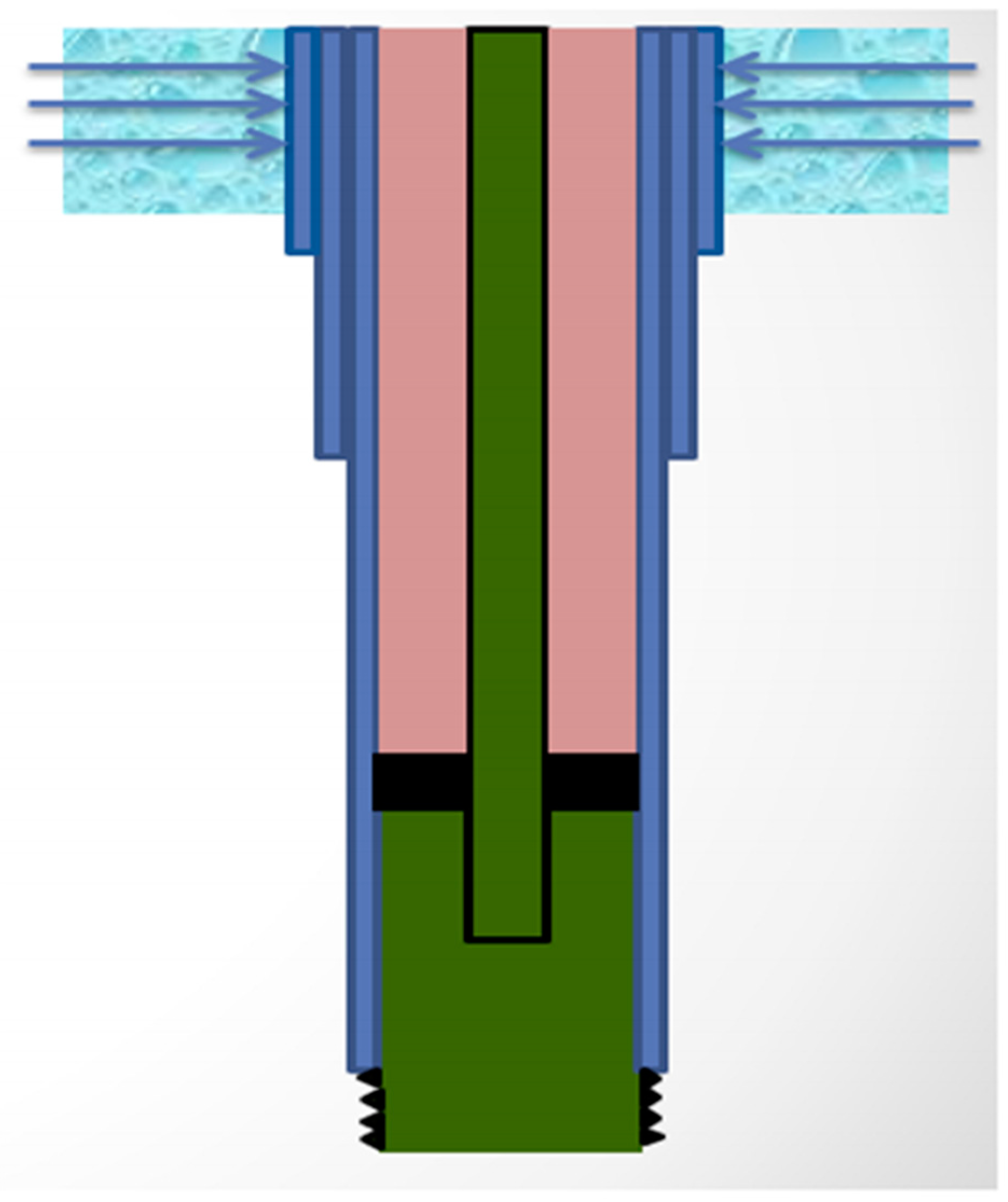
It is imperative that producers have intact well integrity management programs in brown fields in which producing wells are asked to withstand economic production for up to 40 years. Failure to achieve this objective will result in catastrophic economic losses. A good example of this type of loss is the surface leakages affected by the impairment of downhole casings, which result from the corrosion of saline shallow aquifers [6,7]. Figure 1 shows an attack on an active acquirer surrounding an external casing. To better plan for and define future operating regimes and rehabilitation, the capacity to precisely evaluate corrosion rates is essential; such information is a necessary input parameter for any effective corrosion management scenario [6,8,9]. Surface leaks due to corrosion comprise just one example. Surveillance tools can detect casing failures, but only after corrosion occurs.

Corrosion logging is an example of a surveillance tool that offers direct estimation of casing integrity, and thus can be utilized as a predictive tool. The low frequency permits the inspection of more than one tubular and provides a quantitative measure of the remaining wall thickness. When a reduction in metal is encountered while logging, the electromagnetic field induced by the tool will shift, indicating the presence of corrosion (see Figure 1). The tool’s response is further interpreted and converted to a metal loss value. Corrosion logs can then be analyzed to assess the casing integrity and decide on the need for well intervention to prevent potential casing failures (see Figure 2). In large fields, logging all wells requires substantial time, especially given the current resources and manpower. In addition, the limited number of electromagnetic (EM) tools dictates the need for the development of a risk-based candidate selection process. In fact, casing failures and even surface leaks can suddenly strike before a well is logged. The current practice is to rank the candidates according to many factors, including well age, well location, completion quality, and historical integrity. All of these factors are deemed qualitative and solely reliant on the best of judgment of the practitioner.

Corrosion is the gradual loss of the electrons from the surface of a metal, triggering that metal to convert into its ionic shape [10,11,12,13]. The rate of corrosion can be measured by several methods, such as loss of weight and the rate of penetration. Corrosion occurs because metals want to return to the form in which they are found in nature (i.e., oxides, sulfates, or carbonates); such forms are more stable [14]. Downhole assessment of the corrosion rate is the most difficult task in well-integrity surveillance programs. Typically, there are two categories of well downhole corrosion: external and internal [15]. Internal corrosion is triggered when the fluid moving inside the wellbore is naturally corrosive. External corrosion occurs when the outer wall of the tubing comes in contact with the formation. Saline and shallow aquifers are potential sources of external corrosion. Moreover, the cement bond behind the casing being of weak quality can also raise the probability of external corrosion [16,17].

Al-Ajmi et al. [18] used casing corrosion logs such as the EM logging tool to develop a new, risk-based approach to the prediction of oil well bottom-hole leaks. These researchers observed that an EM logging tool alone is not a sufficient estimator of downhole casing leaks caused by corrosion, because this tool is only capable of determining the average value of any external casing corrosion and does not offer its orientation. In their work, the authors developed a new, probabilistic approach that uses the average metal lost as determined by the EM logging tool to assess the possibility of casing failure.

Surveillance programs designed to determine casing integrity are mainly based on annuli and temperature surveys. The tools used for surveillance detect the failure of a casing after it occurs. The purpose of the temperature survey is to locate casing leaks that can lead to a loss of oil production, surface blowouts, and contamination with nearby connected aquifers. Identification and location of casing leaks is imperative to reducing the loss of hydrocarbons and minimizing contamination of nearby connected aquifers. Annuli surveys are regularly conducted to determine annulus pressures. An annulus is the empty space between the casing, tubing, and any pipe with a formation adjacent. In well drilling, an annulus between the casing and formation provides a path for mud to circulate. Corrosion logging tools provide direct measurement of a casing’s integrity, and in many cases can be used as a predictive tool. In corrosion logging, the most common instruments are mechanical, electromagnetic, or ultrasonic.

The main objective of the current research is to present a novel empirical model based on artificial intelligence (AI) and capable of quantifying the corrosion rate in any casing, using its average metal loss percentage data. For the first time, the concept of the average remaining barrier ratio (ARBR) is being presented here, utilized as an input parameter for the new model. This study explores the comparative performances of state-of-the-art and conventional AI techniques in the prediction of corrosion rates. The outcome of this study will assist users of AI techniques in making informed choices regarding the appropriate state-of-the-art methods for use in petroleum production, with the goal of obtaining improved predictions and better decision-making, especially when being faced with limited or sparsely integrated data.

2. Materials and Methods

2.1. Data Analytics

A total of 250 hotspots were collected from 218 wells. Of the 250 data points, 230 were non-leaking; the remaining were considered leaking average metal loss hotspots. The dataset consisted of a variety of completion types, with different casing grades and sizes. The wells produced both oil and water. The ranges of the input parameters were as follows: well age, 2 to 67 years; average metal loss hotspot depth, 9 to 7723 feet; ARBR, 0.095 to 0.908; and corrosion rate, 3.052 to 26.368. The developed AI model was based only on the numerical value for leaking and non-leaking, with 1 representing leaking and 0 representing non-leaking.

The range of the data represented the length of each data interval and arithmetic mean of each implemented parameter. Generally speaking, the standard deviation of a dataset illustrates how that dataset is distributed around its mean value and how much closer the data values are to the mean. The higher the standard deviation from the mean for a specific data type, the more deviated the data are from the mean value. Data skewness explains how symmetrical or skewed the data distribution is in hand. A positive value of skewness indicates that the dataset is skewed to the left, with a longer tail to the right; a negative value of skewness shows that the dataset is skewed to the right, with a longer tail to the left. Skewness values less than −1 or higher than +1 demonstrate that the distribution is highly skewed. Skewness values between −1 and 1 indicate that the data distribution is moderately skewed or approaches symmetricity. The positive Kurtosis values for the current dataset indicate that the data distribution deviated from the normal distribution, with a heavier tail and a sharper peak.

Table 1. Training data statistics for corrosion prediction.

Parameter	Leaking Case (Yes/No)	Average ML, %	Age, Years	Average Remaining Barriers Ratio	Corrosion Rate, MPY
Mean	0.107	0.331	40.664	0.699	9.930
Standard Error	0.028	0.013	0.925	0.013	0.418
Median	0.000	0.300	41.000	0.732	9.644
Mode	0.000	0.230	42.000	0.779	18.227
Standard Deviation	0.310	0.148	10.219	0.142	4.614
Sample Variance	0.096	0.022	104.423	0.020	21.288
Kurtosis	4.745	0.344	0.789	2.155	1.386
Skewness	2.582	0.804	0.216	-1.190	1.051
Range	1.000	0.720	55.000	0.813	23.316
Minimum	0.000	0.100	12.000	0.095	3.052
Maximum	1.000	0.820	67.000	0.908	26.368
Sum	13.000	40.380	4961.000	85.231	1211.481
Count	122.000	122.000	122.000	122.000	122.000

includes the complete statistics for all input and output parameters studied in the present research.

2.2. Average Remaining Barriers Ratio

The ARBR is a dimensionless parameter that takes into account the impacts of various sizes and combinations of casing strings. This parameter is defined as the ratio of the mean number of strings between the corrosive zones (normally water-bearing sands) and the wellbore to the total number of nominal strings at a certain corrosion growth hotspot. The following Equation (1) can be used to compute ARBR:

$$\mathrm{ARBR}=1-\frac{\left[\frac{{\mathrm{T}}_{\mathrm{L}1}}{{\mathrm{T}}_{\mathrm{N}1}}+\frac{{\mathrm{T}}_{\mathrm{L}2}}{{\mathrm{T}}_{\mathrm{N}2}}+\frac{{\mathrm{T}}_{\mathrm{L}3}}{{\mathrm{T}}_{\mathrm{N}3}}+\dots \frac{{\mathrm{T}}_{\mathrm{LX}}}{{\mathrm{T}}_{\mathrm{NX}}}\right]}{\mathrm{X}}$$

(1)

where ARBR is the average remaining barriers ratio (dimensionless), ${\mathrm{T}}_{\mathrm{L}1}$ is the outer string loss of metal thickness (in), ${\mathrm{T}}_{\mathrm{L}2}$ is the second outer string loss of metal thickness (in), ${\mathrm{T}}_{\mathrm{L}3}$ is the third outer string loss of metal thickness (in), ${\mathrm{T}}_{\mathrm{N}1}$ is the outer string’s nominal thickness (in), ${\mathrm{T}}_{\mathrm{N}2}$ is the second outer string’s nominal thickness (in), ${\mathrm{T}}_{\mathrm{N}3}$ is the third outer string’s nominal thickness (in), and $\mathrm{X}$ is the number of strings surrounding the hotspot.

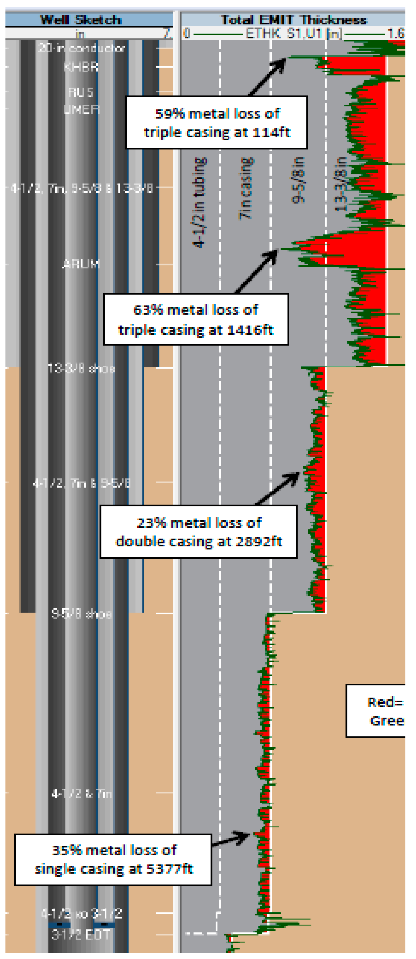
For all practical purposes, a hotspot is defined as any casing depth showing a 12% average metal loss as measured by the electromagnetic induction tool (EMIT) logging device. EMIT gives the average metal loss levels for all installed casing strings. If the tool reads a lower frequency, this means that the penetration is deeper into the casing. The tool detects the average metal loss and changes in casing geometry, regardless of the fluid type. Figure 2 shows a typical response of the EMIT tool.

2.3. Design of the Artificial Neural Networks Model

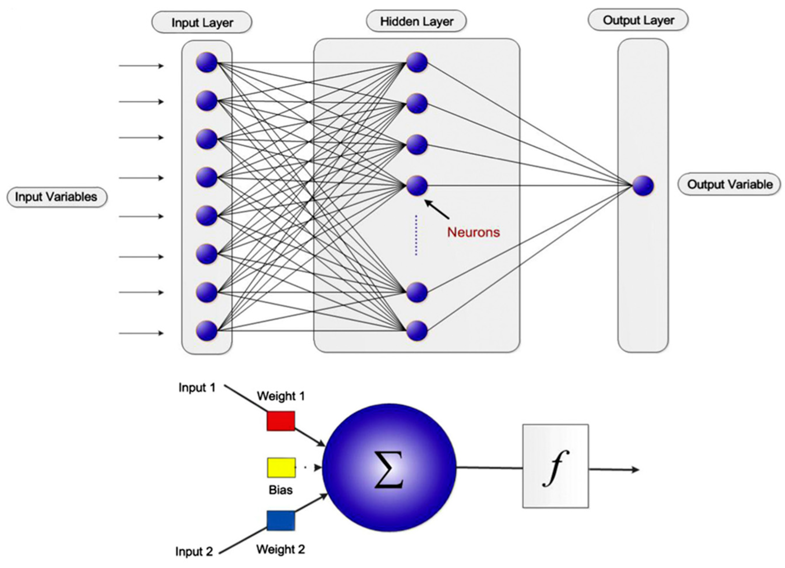
For the last two decades, ANN has served as a useful engineering tool in many applications [19,20]. ANN is an AI technique inspired from the natural features of the biological neurons found in human and animal brains. The fundamental processing units of the ANN model are neurons spread in different layers. Every neuron in the system is linked together to make a network of nodes that form a structure like a biological neural network [21]. A typical ANN model contains an input layer, some number of hidden layers, and an output layer. Signals are received by the input layer. Then, the hidden layer(s) develop relationships among the inputs, and the results are generated at the output layer. Every neuron of a single layer is linked to every neuron in the subsequent layer, and every connection has a related weight [22]. Weights and biases act like coefficients in non-linear equations [23]. The general structure of an ANN model is shown in Figure 3.

In this study, the designed ANN model was developed with three layers: an input layer, a hidden layer, and an output layer. The input layer was comprised of four members. The hidden layer encompassed 20 neurons, and the output layer consisted of one member. The number of neurons in the hidden layer was selected based on the best performance during the training and testing of the modeling phase. A tangential sigmoidal type of activation function was used between the input and hidden layers, and a purely linear type of activation function was used between the hidden and output layers. The learning of ANN model was done with the Levenberg–Marquardt back propagation algorithm. There can be a number of hidden layers between the input and output layers, with varying numbers of neurons. Therefore, to determine the optimum parameters for our problem, an extensive sensitivity analysis was conducted that not only identified the best possible layer/neuron combination, but also provided the most effective training algorithm and transfer function. Consequently, this analysis led us to the best design for an ANN addressing the corrosion rate prediction problem. The complete architecture of the ANN model for predicting corrosion is explained in

Table 2. Developed neural network model for predicting the corrosion rate architecture.

Neural Network Parameter	Range
Number of Inputs	3
Number of Outputs	1
Number of Neurons	20
Number of Hidden Layer(s)	1
Training Algorithm	Levenberg–Marquardt
Learning Rate, $\alpha$	0.12
Hidden-Layer Transfer Function	Tangential sigmoidal
Outer-Layer Transfer Function	Pure linear
Training Ratio	0.7
Testing Ratio	0.15
Validation Ratio	0.15

.

2.4. Design for the Adaptive Network-Based Fuzzy Inference System Model

The adaptive network-based fuzzy inference system (ANFIS) is a type of fuzzy logic (FL) that includes mapping the inputs and outputs of a particular kind, such as in feed-forward neural network systems [24]. Initially developed to model and control ill-defined and uncertain systems [25,26,27], ANFIS models are a blend of FL and neural networks. They comprise a supervised learning technique that uses the Sugeno fuzzy inference system [26]. They operate by applying conventional Boolean logic (i.e., 0’s and 1’s) to describe a principle of truthiness (i.e., values between the completely false, 0, and total truth, 1) [28]. The steps needed for a typical ANFIS model are as follows: (1) defining the input and output variables, (2) declaring fuzzy sets, (3) defining fuzzy rules, and (4) creating and training the network [29,30].

The ANFIS model for the present research was developed with genfis type-2 subtractive clustering (SC). The value of the radius used in SC genfis-2 was selected to be 0.5. The value of the epoch was 500, which represented the number of iterations. The complete architecture of the ANFIS model for predicting corrosion rates is detailed in

Table 3. ANFIS model architecture.

Neural Network Parameter	Range
Number of Inputs	3
Number of Outputs	1
Number of Rules	5
Genfis Type	2
Cluster Radius	0.5
Epoch Size	500

.

The petroleum production property prediction process requires a very high degree of precision; any minor variation from what is anticipated may lead to enormous waste, as well as the loss of man hours and financial investment. Conversely, a slight enhancement of the prediction scenario will produce exponential improvement in present production and exploration projects. Current predictive models are still recognizable in the oil and gas field, but there is an ongoing quest for reliable and improved results.

The modern trend in data analytics and mining is integrating multi-dimensional and multi-modal data for value-added decision-making in petroleum engineering applications. Many commonly used AI techniques have been applied; however, there is still ample room for improvement. Over the years, various AI techniques have attracted attention in a number of geoscience and engineering applications. Many successful implementations of this science in real oil and gas cases have attracted considerable interest, especially those applying these techniques to predict challenging industry parameters. Some areas of petroleum engineering in which AI techniques have introduced new innovations include: permeability porosity relationship predictions [20,31], hydraulic flow unit identification [32], geomechanics parameters estimation [33,34], geophysical well logs estimation [35,36], drilling parameters estimation [37,38], water saturation prediction [39], enhanced oil recovery [40], and many others. Common traditional AI techniques applied in petroleum engineering applications include ANNs, functional networks (FNs), support vector machines (SVMs), decision trees, and FL. These techniques have various advantages and disadvantages that impose structural and technical limitations, affecting their predictive performance; these make their applications inappropriate in specified situations such as conditions of limited, sparse, or missing data [41]. A rigorous comparative study that determines the applicability and performance of state-of-the-art AI techniques in petroleum production parameter prediction is sorely needed.

2.5. Feature Selection Using a Multivariate Linear Regression System

Every AI model is data-driven, including all of the available attributes acting as input parameters. These do not generate useful results, so it is always important to determine which input parameters are the strongest contributors and the most influential. In the present research, a Pearson’s correlation coefficient (CC) was utilized to determine that relationship, in terms of the CC between input and output parameters. The CC input and output values were determined using Equation (2).

$$\mathrm{CC}=\frac{\mathrm{k}{\displaystyle \sum }\mathrm{xy}-\left({\displaystyle \sum }\mathrm{x}\right)\left({\displaystyle \sum }\mathrm{y}\right)}{\sqrt{\mathrm{k}\left({\displaystyle \sum }{\mathrm{x}}^2\right)-{\left({\displaystyle \sum }\mathrm{y}\right)}^2}\sqrt{\mathrm{k}\left({\displaystyle \sum }{\mathrm{b}}^2\right)-{\left({\displaystyle \sum }\mathrm{b}\right)}^2}}$$

(2)

The CC value for a pair of variables always lies between −1 and 1. A CC value close to −1 shows a strong inverse relationship between the pair of variables, while a value close to 1 indicates a strong direct relationship between the two. A CC value of zero demonstrates that no relationship exists between the two variables.

2.6. Goodness-of-Fit Tests

To determine the strength of the proposed model, several goodness-of-fit criteria were used, such as the average absolute percentage error (AAPE) given by Equation (3), root mean squared error (RMSE) given by Equation (4), and coefficient of determination (R²) given by Equation (5).

Average Absolute Percentage Error

$$\mathrm{AAPE}=\frac{{\displaystyle \sum }\left|\left({\mathrm{a}}_{\mathrm{i}}-{\mathrm{b}}_{\mathrm{i}}\right)\right|\times \frac{100}{{\mathrm{a}}_{\mathrm{i}}}}{\mathrm{n}}$$

(3)

Root Mean Square Error

$$\mathrm{RMSE}=\sqrt{\frac{{\displaystyle \sum }{\left({\mathrm{a}}_{\mathrm{i}}-{\mathrm{b}}_{\mathrm{i}}\right)}^2}{\mathrm{n}}}$$

(4)

where $\mathrm{a}$ is the actual value and b is the predicted value, and n is the total number of data points.

Coefficient of Determination

$${\mathrm{R}}^2={\left(\frac{\mathrm{k}{\displaystyle \sum }\mathrm{xy}-\left({\displaystyle \sum }\mathrm{x}\right)\left({\displaystyle \sum }\mathrm{y}\right)}{\sqrt{\mathrm{k}\left({\displaystyle \sum }{\mathrm{x}}^2\right)-{\left({\displaystyle \sum }\mathrm{y}\right)}^2}\sqrt{\mathrm{k}\left({\displaystyle \sum }{\mathrm{b}}^2\right)-{\left({\displaystyle \sum }\mathrm{b}\right)}^2}}\right)}^2$$

(5)

where x and y are the two variables and k is the total number of data points.

3. Mathematical Model for Predicting the Corrosion Rate

A major outcome of this work is the development of an empirical model using a trained neural network based on a set of weights and biases related to both the hidden input and output layers. The weights and biases corresponding to their neurons are shown in

Table 4. Weights and biases of the ANN model for predicting the corrosion rate (in mills per year).

Hidden Layer Neurons (N)	Weights Between Input and Hidden Layers (W1)				Weights Between Hidden and Output Layers (W1)	Hidden Layer Bias (b1)	Output Layer Bias (b2)
	Leak	ML, %	AGE, Years	ARBR
1	−0.8056	2.0361	−0.7806	1.5471	0.5893	3.2630	0.3366
2	0.7801	−2.2259	−1.1987	−1.4638	−0.7081	−2.5455
3	−1.1518	1.9819	0.5252	1.2399	−0.2656	2.8491
4	−2.2960	−0.0809	0.2676	−2.3103	−0.8699	1.8388
5	−2.7286	1.1579	1.0355	0.2912	0.2949	1.1351
6	2.4246	−0.5461	0.9256	0.6130	−0.4835	−1.6147
7	1.4496	2.5089	1.4569	0.0958	1.0998	−1.2605
8	1.3588	−0.3056	−1.7989	−1.1340	1.0042	−1.4414
9	−1.9955	−0.3955	−1.7329	−0.6282	1.3636	−0.0667
10	2.6130	−0.8845	1.0068	−0.3291	−0.5042	−0.6139
11	0.3650	1.7472	3.1860	1.1018	−0.9459	0.4697
12	−0.6945	−1.5393	−0.9785	−1.1627	1.0357	−0.9896
13	0.1043	1.8686	−0.6753	−2.2764	−0.0062	0.8773
14	−2.1720	−0.4880	2.0517	0.9744	−1.3560	−1.1831
15	−0.4380	−2.0103	−3.1879	−0.2956	−1.1222	−1.5927
16	1.1553	−2.1156	−1.5031	−1.5825	−1.0756	1.9112
17	0.7408	2.1181	1.6252	0.7625	−0.2558	2.1355
18	0.1500	0.4894	−2.4771	1.6431	−0.5102	2.0059
19	−1.9882	−0.4098	0.3490	−1.9301	−0.3645	−2.9039
20	1.2717	2.3014	0.9231	1.1425	0.9099	2.9353

; those linked with the hidden input layer are characterized by w₁, whereas those linked with the hidden output layer are called w₂. Furthermore, the hidden input and output layer biases are b₁ and b₂, respectively. The new empirical correlation developed using ANN for the water saturation estimation is given by Equation (6):

$${\mathrm{CR}}_{\mathrm{n}}=\left[{\displaystyle \sum }_{\mathrm{i}=1}^{\mathrm{N}}{\mathrm{w}}_{2_{\mathrm{i}}}\left(\frac{2}{1+{\mathrm{e}}^{-2\left({\mathrm{w}}_{1_{\mathrm{i},1}}{\mathsf{\rho }}_{\mathrm{n}}+{\mathrm{w}}_{1_{\mathrm{i},2}}{\mathrm{ML}}_{\mathrm{n}}+{\mathrm{w}}_{1_{\mathrm{i},3}}{\mathrm{Y}}_{\mathrm{n}}+{\mathrm{w}}_{1_{\mathrm{i},4}}{\mathrm{ARBR}}_{\mathrm{n}}+{\mathrm{b}}_{1_{\mathrm{i}}}\right)}}-1\right)\right]+{\mathrm{b}}_2$$

(6)

where ${\mathsf{\rho }}_{\mathrm{n}}$ is the normalized value for the leaking/non-leaking case, ${\mathrm{ML}}_{\mathrm{n}}$ is the normalized value of the metal loss, ${\mathrm{Y}}_{\mathrm{n}}$ is the normalized value of the age of the casing, and ${\mathrm{ARBR}}_{\mathrm{n}}$ is the normalized value of ARBR, N is the total number of neurons from the trained model, w₁ and w₂ are the weights between input/hidden layers, and b₁ and b₂ are the biases in the input/hidden layers.

Procedure for Using the New Empirical Correlation for the Corrosion Rate

Following are the three steps to follow when adopting the new equation to predict a corrosion rate.

Step 1: Normalize the input parameters to be between −1 and 1. The input parameters (i.e., casing leaks, metal loss percentage, age of casing, and ARBR) are denoted here by “Input”. The general equation for normalization is Equation (7):

$${\mathrm{Input}}_{\mathrm{norm}}=\frac{\left({\mathrm{Input}}_{\max }-{\mathrm{Input}}_{\min }\right)\left(\mathrm{X}-{\mathrm{X}}_{\min }\right)}{{\mathrm{X}}_{\max }-{\mathrm{X}}_{\min }}+{\mathrm{Input}}_{\min }$$

(7)

$\mathrm{where} {\mathrm{Input}}_{\min }=-1$ and ${\mathrm{Input}}_{\max }=1$, X is the input parameter, X_min is the minimum value of the trained input parameter, and X_max is the maximum value of the trained input parameter. X_min and X_max are given in Table 1. To perform the normalization for casing leaks, metal loss percentage, age of casing, and ARBR, Equations (8)–(11) were used:

$${\mathsf{\rho }}_{\mathrm{n}}=2\times \left(\frac{\mathsf{\rho }-0}{1-0}\right)-1$$

(8)

$${\mathrm{ML}}_{\mathrm{n}}=2\times \left(\frac{\mathrm{ML}-0.1}{0.82-0.1}\right)-1$$

(9)

$$y_{\mathrm{n}}=2\times \left(\frac{y-12}{67-12}\right)-1$$

(10)

$${\mathrm{ARBR}}_{\mathrm{n}}=2\times \left(\frac{\mathrm{ARBR}-0.095}{0.908-0.095}\right)-1$$

(11)

Step 2: The weights and biases given in Table 4 were necessary to apply Equation (6). The sequence of parameters going into the model was as follows: casing leaks, metal loss percentage, age of casing, and ARBR.

Step 3: Equation (6) gives the corrosion rate in a normalized form, within the range of −1 to 1. To de-normalize the corrosion rate and transform it into a real-value form, Equation (13) can be used:

$$\mathrm{CR}=\frac{\left(26.368-3.052\right)\left({\mathrm{CR}}_{\mathrm{n}}+1\right)}{2}+3.052$$

(12)

$$\mathrm{CR}=11.652\times {\mathrm{CR}}_{\mathrm{n}}+14.72$$

(13)

4. Results and Discussion

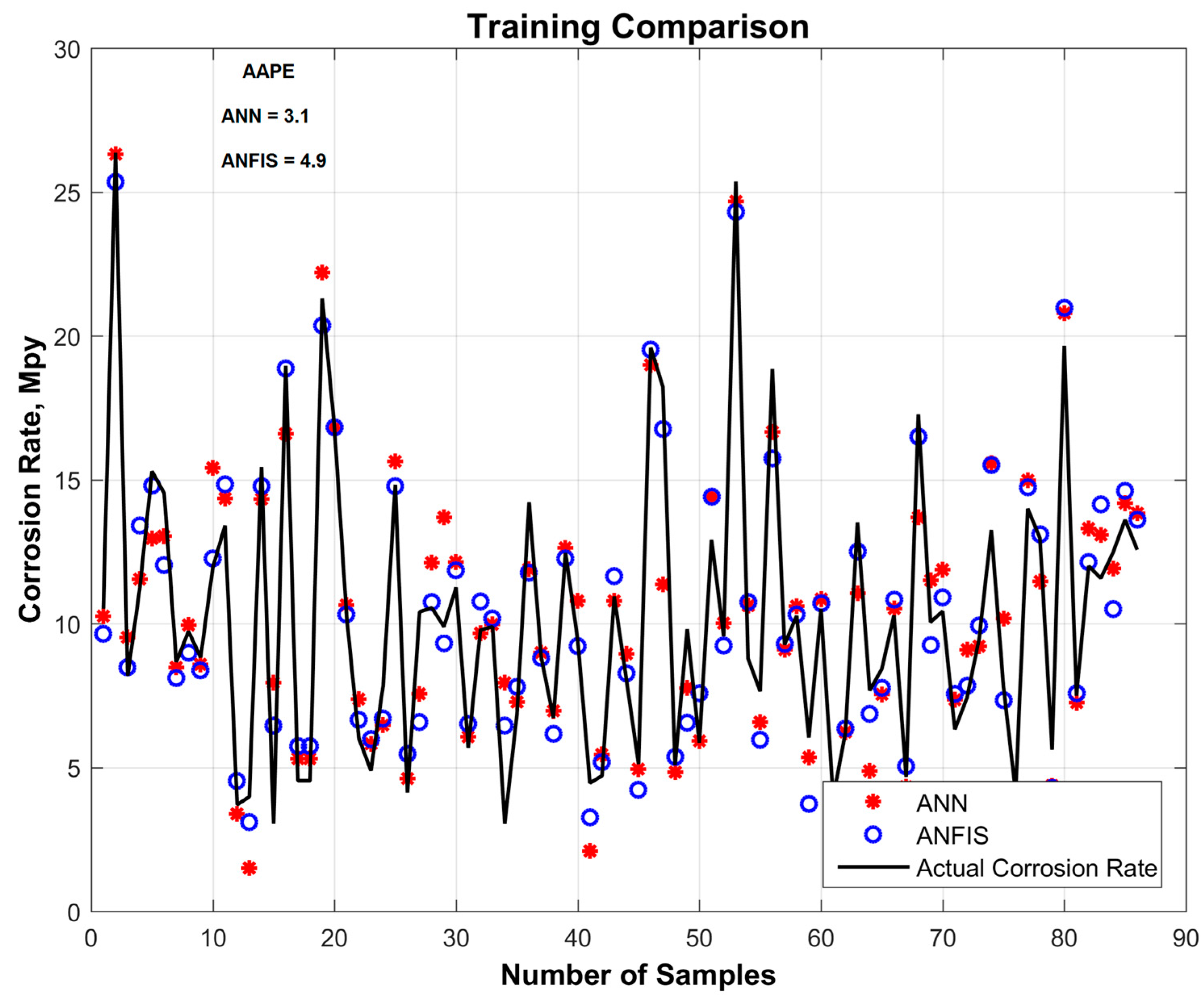
A total of 250 data points were divided randomly into two sets, at a proportion of 0.7 to 0.3. The set with 70% of the data (i.e., 175 data points) was utilized for training the models, and the second set, with 30% of the data (i.e., 75 data points), was used to test the prediction capabilities of the trained models. Two AI techniques, ANN and ANFIS, were implemented to develop the models and predict the corrosion rate. A comparison was made between these techniques, based on the lowest AAPE and highest R² for the actual and predicted values. For ANN, several runs were executed with various values for the model parameters. At every run, the parameters of learning rate, number of hidden layers with a corresponding number of neurons, and different transfer functions were all changed. For ANFIS, in genfis-2, the sensitivity of the cluster radii was performed such that it reached the optimum model. The proposed model(s) were tuned by optimizing their several variables via particle swarm optimization.

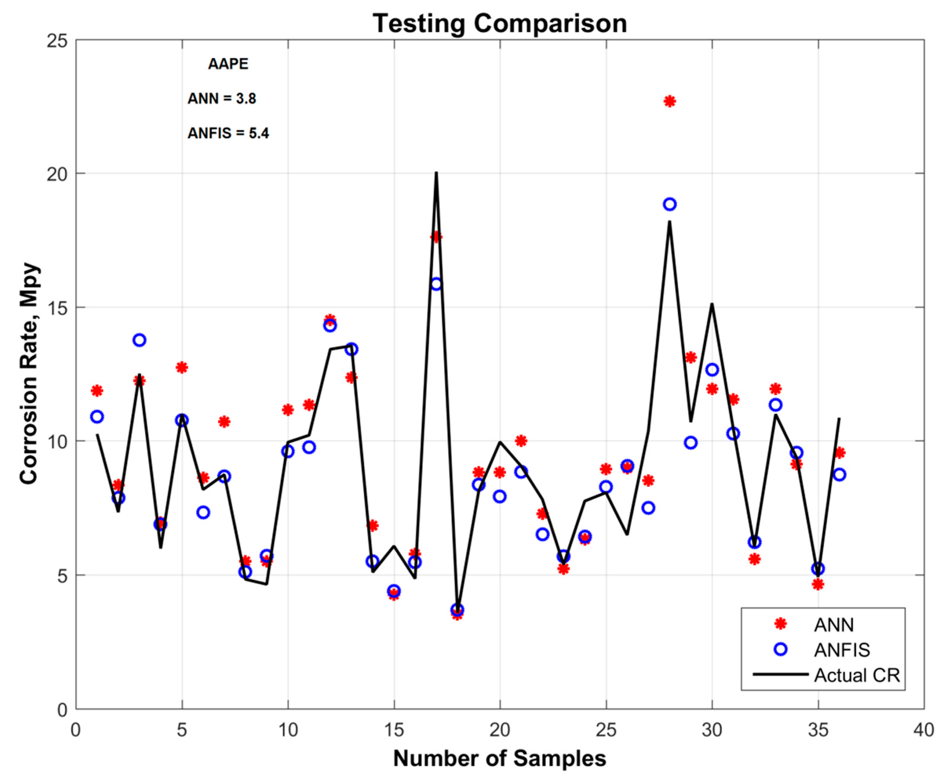
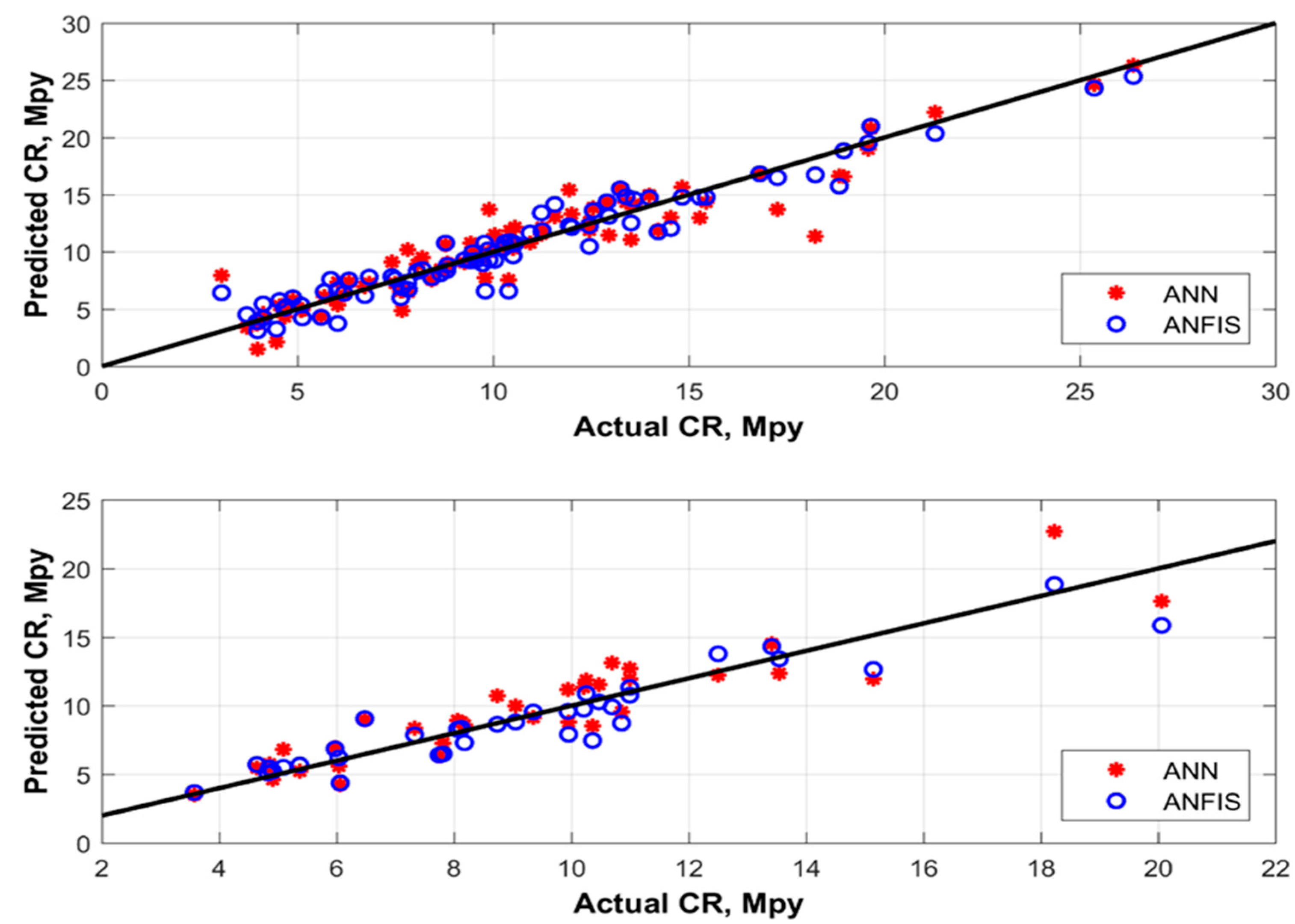
On a training dataset, ANN predicted the corrosion rate with an AAPE of 3.1, and ANFIS predicted the corrosion rate with an AAPE of 4.9. On the testing dataset, ANN predicted the corrosion rate with an AAPE of 3.8, and ANFIS predicted it with an AAPE of 5.4. Figure 4 and Figure 5 show a comparison of the corrosion rates predicted by ANN and ANFIS, during both the training and testing phases of modeling. Figure 6 shows a cross-plot comparison of the ANN and ANFIS techniques for predicting corrosion rates. To prevent the model from becoming stuck on a local minima, more than 50,000 realizations were performed with the initialization of different sets of weights and biases during training of the prediction modeling. After training, the optimum weights and biases from the trained model were extracted; these are given in Table 4.

5. Validation of the Proposed Model

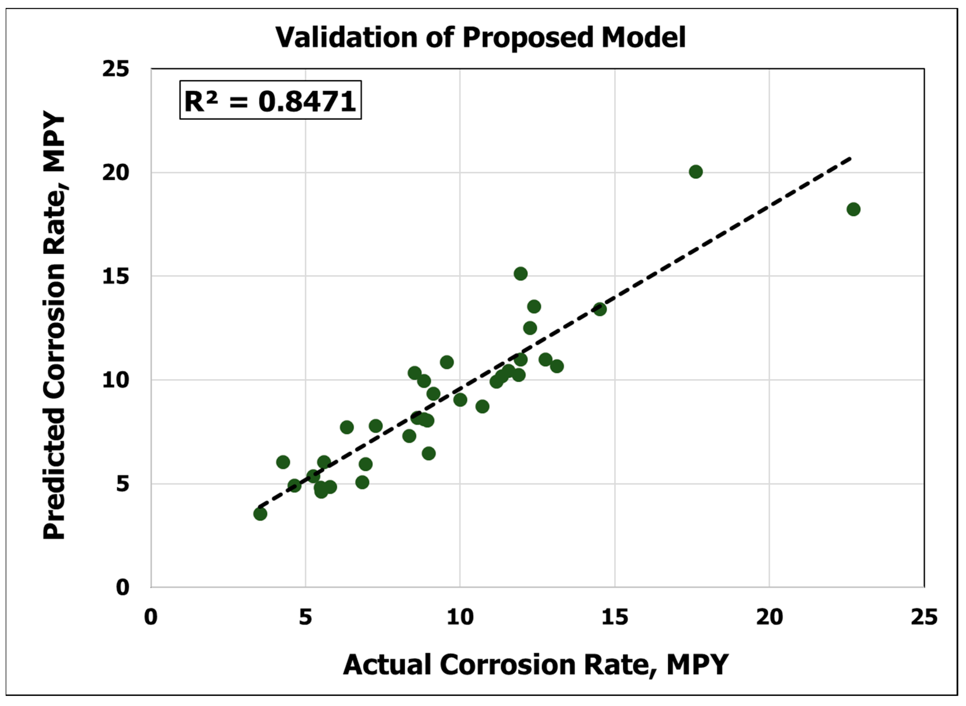
To validate the new model, a variety of datasets from different wells were obtained. The data gathered via the EMIT logging tool response were then digitized.

Table 5. Performance comparison of different AI techniques.

ID	Leaking Case (Yes/No)	Average ML%	Age, Years	Average Remaining Barriers Ratio	Corrosion Rate, MPY	ANN	APE	AAPE
							ANN	ANN
1	1	0.59	45	0.455	10.253	11.877	15.839	13.919
2	0	0.3	45	0.744	7.327	8.347	13.921
3	0	0.21	22	0.789	12.505	12.241	2.111
4	0	0.25	46	0.787	5.973	6.938	16.156
5	0	0.4	40	0.658	10.990	12.738	15.905
6	0	0.24	37	0.768	8.173	8.607	5.310
7	0	0.31	39	0.736	8.736	10.715	22.653
8	0	0.18	41	0.847	4.825	5.488	13.741
9	0	0.19	45	0.838	4.640	5.493	18.384
10	0	0.38	42	0.676	9.943	11.162	12.260
11	0	0.39	42	0.668	10.205	11.346	11.181
12	0	0.47	40	0.577	13.419	14.505	8.093
13	1	0.53	43	0.522	13.546	12.370	8.682
14	0	0.2	34	0.801	5.088	6.821	34.061
15	0	0.16	41	0.882	6.064	4.257	29.799
16	0	0.19	42	0.842	4.850	5.773	19.031
17	0	0.47	37	0.571	20.058	17.612	12.195
18	0	0.13	40	0.889	3.572	3.525	1.316
19	0	0.34	46	0.710	8.123	8.818	8.556
20	0	0.22	28	0.786	9.955	8.818	11.421
21	0	0.42	53	0.625	9.050	9.994	10.431
22	0	0.23	41	0.814	7.809	7.260	7.030
23	0	0.25	55	0.771	5.373	5.231	2.643
24	0	0.22	45	0.820	7.744	6.318	18.414
25	0	0.33	45	0.719	8.059	8.937	10.895
26	0	0.31	44	0.730	6.475	8.965	38.456
27	0	0.25	37	0.780	10.365	8.518	17.820
28	0	0.68	41	0.366	18.227	22.696	24.519
29	0	0.36	37	0.693	10.693	13.114	22.641
30	1	0.62	45	0.429	15.142	11.936	21.173
31	0	0.4	42	0.658	10.467	11.544	10.289
32	0	0.27	56	0.737	6.041	5.583	7.582
33	0	0.42	42	0.637	10.990	11.941	8.653
34	0	0.27	33	0.761	9.347	9.133	2.290
35	0	0.24	58	0.779	4.912	4.636	5.619
36	0	0.24	28	0.767	10.860	9.555	12.017

shows the input parameters, actual corrosion rates, and predicted corrosion rates from the ANN model. With a new dataset, the proposed model yielded a perfect prediction by giving a coefficient of determination of 0.85, AAPE of 13 %, and RMSE of 3.7, as shown in Figure 7 and

Table 6. Validation results of the ANN-based model.

AAPE	RMSE	CC	R2
13	3.7	0.92	0.847

. The results obtained from the validation confirmed the generalization and robustness of the new model. Thus, it can be argued that the new model is capable of make predictions with any new dataset, so long as the inputs are within the range defined in Table 1.

6. Conclusions

This paper presents an ANN-based empirical model that can be used as a predictive tool when implementing wellbore integrity management strategies, leading to more sustained environmental protection. The imprecise results produced by the EMIT logging tool can be focused by studying the average metal loss measurements across the leaking and non-leaking metal loss hotspots, and presenting how the ARBR concept normalizes the impact of multiple casings sizes, grades, combinations, and thicknesses. The following conclusion can also be drawn from this study.

• Machine learning techniques have successfully been shown to predict corrosion rates with a correlation of determination of approximately 94% in the case of ANN, and 96% when using ANFIS.
• A new empirical model for estimating corrosion rates has been proposed that can be applied to any case in which the input parameters are within the developed model’s range; this can be accomplished without the need for intricate software.
• ANFIS provides slightly better results. However, the estimation is not greatly affected if ANN is used. Furthermore, neural networks have been used to produce a practical working equation.
• Additional techniques like SVMs and FNs should be explored to investigate the possibility of gaining better results.

References

- Kermani, M.B.; Harrop, D. The Impact of Corrosion on Oil and Gas Industry. SPE Prod. Facil. 1996, 11, 186–190. [Google Scholar] [CrossRef]
- Davies, R.J.; Almond, S.; Ward, R.S.; Jackson, R.B.; Adams, C.; Worrall, F.; Herringshaw, L.G.; Gluyas, J.G.; Whitehead, M.A. Oil and gas wells and their integrity: Implications for shale and unconventional resource exploitation. Mar. Pet. Geol. 2014, 56, 239–254. [Google Scholar] [CrossRef]
- Considine, T.J.; Watson, R.W.; Considine, N.B.; Martin, J.P. Environmental regulation and compliance of Marcellus Shale gas drilling. Environ. Geosci. 2013, 20, 1–16. [Google Scholar] [CrossRef]
- Ingraffea, A.R.; Wells, M.T.; Santoro, R.L.; Shonkoff, S.B.C. Assessment and risk analysis of casing and cement impairment in oil and gas wells in Pennsylvania, 2000–2012. Proc. Natl. Acad. Sci. USA 2014, 111, 10955–10960. [Google Scholar] [CrossRef] [PubMed]
- Klassen, W. Secondary Intervention of Blow Out Preventers. In Proceedings of the SPE Offshore Europe Oil and Gas Conference and Exhibition, Aberdeen, UK, 3–6 September 2013. [Google Scholar]
- Al-Ashhab, J.; Afzal, M.; Emenike, C.O. Well Integrity Management System (WIMS). In Proceedings of the Abu Dhabi International Conference and Exhibition, Abu Dhabi, UAE, 10–13 October 2004. [Google Scholar]
- Chatriwala, S.A.; Al-Subaie, F.M.; Al-Shehri, D.A.; Soremi, A.X.; Reaux, J. First Saudi Aramco Use of Retrievable Downhole Pressure and Temperature Gauges Monitoring System: A Cost Effective Technology Solution to Manage Maturing Oil and Gas Fields. In Proceedings of the SPE Saudi Arabia Section Technical Symposium, Al-Khobar, Saudi Arabia, 9–11 May 2009. [Google Scholar]
- Al Khamis, M.N.; Al Khalewi, F.T.; Al Hanabi, M.; Al Yateem, K.; Al Qatari, A.; Al Muailu, H. A Comprehensive Approach of Well Integrity Surveillance. In Proceedings of the International Petroleum Technology Conference; International Petroleum Technology Conference, Kuala Lumpur, Malaysia, 10–12 December 2014. [Google Scholar]
- Stokes, P.; Sandana, D.; Jones, L. Corrosion Management—it’s all gone holistic. In Proceedings of the SPE International Oilfield Corrosion Conference and Exhibition, Aberdeen, UK, 12–13 May 2014. [Google Scholar]
- AlAjmi, M.D.; Abdulraheem, A.; Mishkhes, A.T.; Al-Shammari, M.J. Profiling Downhole Casing Integrity Using Artificial Intelligence. In Proceedings of the SPE Digital Energy Conference and Exhibition, The Woodlands, TX, USA, 3–5 March 2015. [Google Scholar]
- Brill, T.M.; Demichel, C.; Nichols, E.A.; Zapata Bermudez, F. Electromagnetic Casing Inspection Tool for Corrosion Evaluation. In Proceedings of the International Petroleum Technology Conference, Bangkok, Thailand, 15–17 November 2011. [Google Scholar]
- Brill, T.M.; Le Calvez, J.-L.; Demichel, C.; Nichols, E.; Bermudez, F.Z. Quantitative Corrosion Assessment with an EM Casing Inspection Tool. In Proceedings of the SPE/DGS Saudi Arabia Section Technical Symposium and Exhibition, Al-Khobar, Saudi Arabia, 15–18 May 2011. [Google Scholar]
- Rahman, M.; Zahir, M.; Haq, M.; Shehri, D.; Kumar, A. Corrosion Inhibition Properties of Waterborne Polyurethane/Cerium Nitrate Coatings on Mild Steel. Coatings 2018, 8, 34. [Google Scholar] [CrossRef]
- McCafferty, E. Validation of corrosion rates measured by the Tafel extrapolation method. Corros. Sci. 2005, 47, 3202–3215. [Google Scholar] [CrossRef]
- Tems, R.D. Downhole corrosion. In Trends in Oil and Gas Corrosion Research and Technologies; Elsevier: Amsterdam, The Netherlands, 2017; pp. 79–94. [Google Scholar]
- Papavinasam, S. Monitoring—Internal Corrosion. In Corrosion Control in the Oil and Gas Industry; Elsevier: Amsterdam, The Netherlands, 2014; pp. 425–528. [Google Scholar]
- Papavinasam, S. The Oil and Gas Industry. In Corrosion Control in the Oil and Gas Industry; Elsevier: Amsterdam, The Netherlands, 2014; pp. 1–39. [Google Scholar]
- Al-Ajmi, M.D.; Al-Shehri, D.; Mahmoud, M.; Al-Hajri, N.M. Risk-Based Approach to Evaluate Casing Integrity in Upstream Wells. J. Energy Resour. Technol. 2018, 140, 122901. [Google Scholar] [CrossRef]
- Rammay, M.H.; Abdulraheem, A. PVT correlations for Pakistani crude oils using artificial neural network. J. Pet. Explor. Prod. Technol. 2016, 7, 217–233. [Google Scholar] [CrossRef]
- Nooruddin, H.A.; Anifowose, F.; Abdulraheem, A. Applying Artificial Intelligence Techniques to Develop Permeability Predictive Models using Mercury Injection Capillary-Pressure Data. In Proceedings of the SPE Saudi Arabia Section Technical Symposium and Exhibition, S Al-Khobar, Saudi Arabia, 19–22 May 2013. [Google Scholar]
- Hinton, G.E.; Osindero, S.; Teh, Y.-W. A Fast Learning Algorithm for Deep Belief Nets. Neural Comput. 2006, 18, 1527–1554. [Google Scholar] [CrossRef] [PubMed]
- Lippmann, R. Book Review: “Neural Networks, A Comprehensive Foundation”, by Simon Haykin. Int. J. Neural Syst. 1994, 05, 363–364. [Google Scholar] [CrossRef]
- Vineis, P.; Rainoldi, A. Neural networks and logistic regression: Analysis of a case-control study on myocardial infarction. J. Clin. Epidemiol. 1997, 50, 1309–1310. [Google Scholar] [CrossRef]
- Tariq, Z.; Elkatatny, S.; Mahmoud, M.; Ali, A.Z.; Abdulraheem, A. A New Approach to Predict Failure Parameters of Carbonate Rocks using Artificial Intelligence Tools. In Proceedings of the SPE Kingdom of Saudi Arabia Annual Technical Symposium and Exhibition, Dammam, Saudi Arabia, 24–27 April 2017. [Google Scholar]
- Jang, J.-S.R.; Sun, C.-T. Neuro-fuzzy modeling and control. Proc. IEEE 1995, 83, 378–406. [Google Scholar] [CrossRef]
- Jang, J.-S.R. ANFIS: adaptive-network-based fuzzy inference system. IEEE Trans. Syst. Man. Cybern. 1993, 23, 665–685. [Google Scholar] [CrossRef]
- Jang, J.-S.R. Input selection for ANFIS learning. In Proceedings of the IEEE 5th International Fuzzy Systems, New Orleans, LA, USA, 11 September 1996; Volume 2, pp. 1493–1499. [Google Scholar]
- Ebrahimi, M.; Sajedian, A. Use of Fuzzy Logic for Predicting Two Phase Inflow Performance Relationship of Horizontal Oil Wells. In Proceedings of the Trinidad and Tobago Energy Resources Conference, Port of Spain, Trinidad and Tobago, 27–30 June 2010; ISBN 978-1-61738-885-9. [Google Scholar]
- Walia, N.; Singh, H.; Sharma, A. ANFIS: Adaptive Neuro-Fuzzy Inference System—A Survey. Int. J. Comput. Appl. 2015, 123, 32–38. [Google Scholar] [CrossRef]
- Tahmasebi, P.; Hezarkhani, A. A hybrid neural networks-fuzzy logic-genetic algorithm for grade estimation. Comput. Geosci. 2012, 42, 18–27. [Google Scholar] [CrossRef] [PubMed]
- Abdulraheem, A.; Sabakhy, E.; Ahmed, M.; Vantala, A.; Raharja, P.D.; Korvin, G. Estimation of Permeability from Wireline Logs in a Middle Eastern Carbonate Reservoir Using Fuzzy Logic. In Proceedings of the SPE Middle East Oil and Gas Show and Conference, Manama, Bahrain, 11–14 March 2007. [Google Scholar]
- Shujath Ali, S.; Hossain, M.E.; Hassan, M.R.; Abdulraheem, A. Hydraulic Unit Estimation From Predicted Permeability and Porosity Using Artificial Intelligence Techniques. In Proceedings of the North Africa Technical Conference and Exhibition, Cairo, Egypt, 15–17 April 2013. [Google Scholar]
- Abdulraheem, A.; Ahmed, M.; Vantala, A.; Parvez, T. Prediction of Rock Mechanical Parameters for Hydrocarbon Reservoirs Using Different Artificial Intelligence Techniques. In Proceedings of the SPE Saudi Arabia Section Technical Symposium, Al-Khobar, Saudi Arabia, 9–11 May 2009. [Google Scholar]
- Tariq, Z.; Abdulraheem, A.; Mahmoud, M.; Ahmed, A. A Rigorous Data-Driven Approach to Predict Poisson’s Ratio of Carbonate Rocks Using a Functional Network. Petrophysics—SPWLA J. Form. Eval. Reserv. Descr. 2018, 59, 761–777. [Google Scholar]
- Tariq, Z.; Elkatatny, S.; Mahmoud, M.; Abdulraheem, A. A Holistic Approach to Develop New Rigorous Empirical Correlation for Static Young’s Modulus. In Proceedings of the Abu Dhabi International Petroleum Exhibition & Conference, Abu Dhabi, UAE, 7–10 November 2016. [Google Scholar]
- Tariq, Z.; Mahmoud, M.A.; Abdulraheem, A.; Al-Shehri, D.A. On Utilizing Functional Network to Develop Mathematical Model for Poisson’s Ratio Determination. In Proceedings of the 52nd U.S. Rock Mechanics/Geomechanics Symposium, Seattle, WA, USA, 23–26 June 2018. [Google Scholar]
- Al-Azani, K.; Elkatatny, S.; Abdulraheem, A.; Mahmoud, M.; Al-Shehri, D. Real Time Prediction of the Rheological Properties of Oil-Based Drilling Fluids Using Artificial Neural Networks. In Proceedings of the SPE Kingdom of Saudi Arabia Annual Technical Symposium and Exhibition, Dammam, Saudi Arabia, 23–26 April 2018. [Google Scholar]
- Elzenary, M.; Elkatatny, S.; Abdelgawad, K.Z.; Abdulraheem, A.; Mahmoud, M.; Al-Shehri, D. New Technology to Evaluate Equivalent Circulating Density While Drilling Using Artificial Intelligence. In Proceedings of the SPE Kingdom of Saudi Arabia Annual Technical Symposium and Exhibition, Dammam, Saudi Arabia, 23–26 April 2018. [Google Scholar]
- Adebayo, A.R.; Abdulraheem, A.; Olatunji, S.O. Artificial intelligence based estimation of water saturation in complex reservoir systems. J. Porous Media 2015, 18, 893–906. [Google Scholar] [CrossRef]
- Tariq, Z.; Mahmoud, M.; Al-Shehri, D.; Sibaweihi, N.; Sadeed, A.; Hossain, M.E. A Stochastic Optimization Approach for Profit Maximization Using Alkaline-Surfactant-Polymer Flooding in Complex Reservoirs. In Proceedings of the SPE Kingdom of Saudi Arabia Annual Technical Symposium and Exhibition, Dammam, Saudi Arabia, 23–26 April 2018. [Google Scholar]
- Anifowose, F.; Adeniye, S.; Abdulraheem, A. Recent advances in the application of computational intelligence techniques in oil and gas reservoir characterisation: A comparative study. J. Exp. Theor. Artif. Intell. 2014, 26, 551–570. [Google Scholar] [CrossRef]
Figure 1.
View of external corrosion attacking an outer casing string on a well with an active aquifer.
Figure 2.
Typical response of the EMIT logging tool showing the metal loss percentage.
Figure 3.
Typical structure of an ANN.
Figure 4.
Training comparison of different AI techniques for predicting corrosion rates.
Figure 5.
Testing comparison of different AI techniques for predicting corrosion rates.
Figure 6.
Training and testing cross-plot comparison of different AI techniques for predicting corrosion rates.