Integrating Biophysical and Sociocultural Methods for Identifying the Relationships between Ecosystem Services and Land Use Change: Insights from an Oasis Area

 ,
,  , and
, and
Abstract
:1. Introduction
2. Materials and Methods
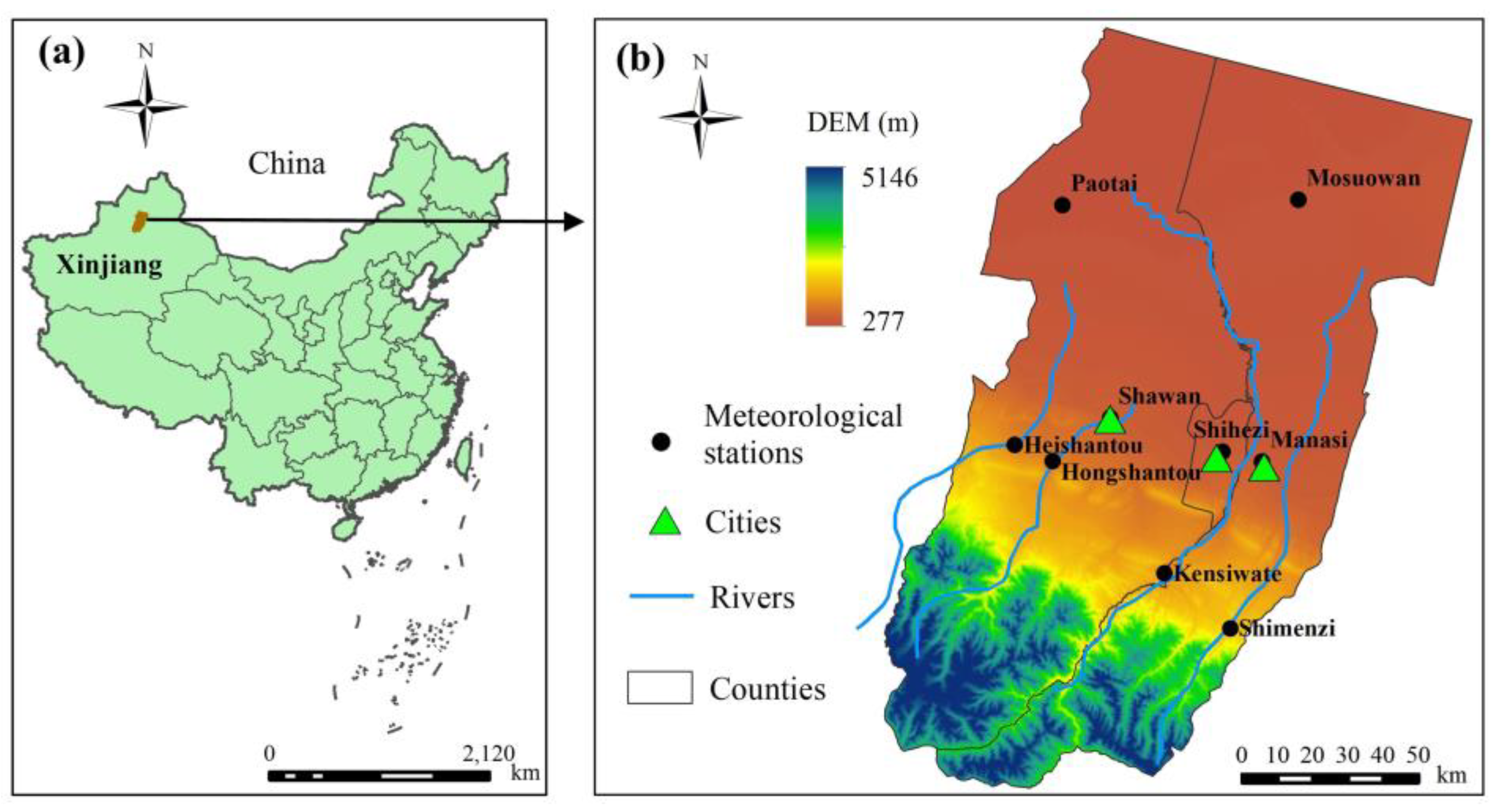
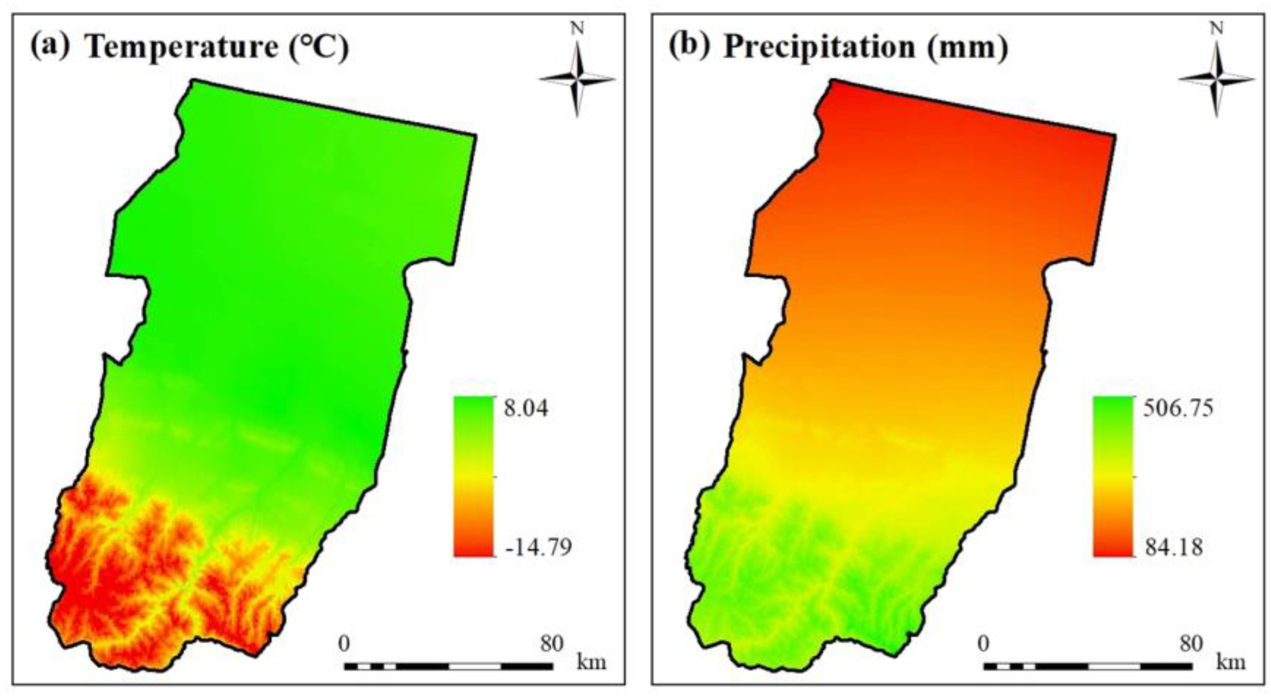
2.1. Study Area
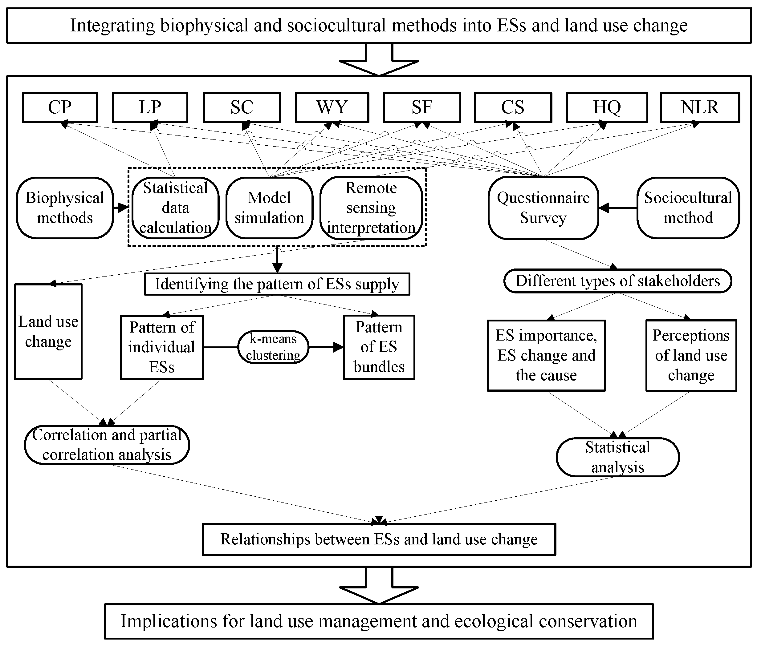
2.2. Research Route
2.3. Ecosystem Services Supply: Biophysical Methods
2.3.1. Selection of Key Ecosystem Services
2.3.2. Data Requirements and Preparation
2.3.3. Mapping of Individual Ecosystem Services Supply
2.3.4. Identification and Mapping of Ecosystem Service Bundles
2.4. Questionnaire Survey
2.5. Data Analysis
3. Results
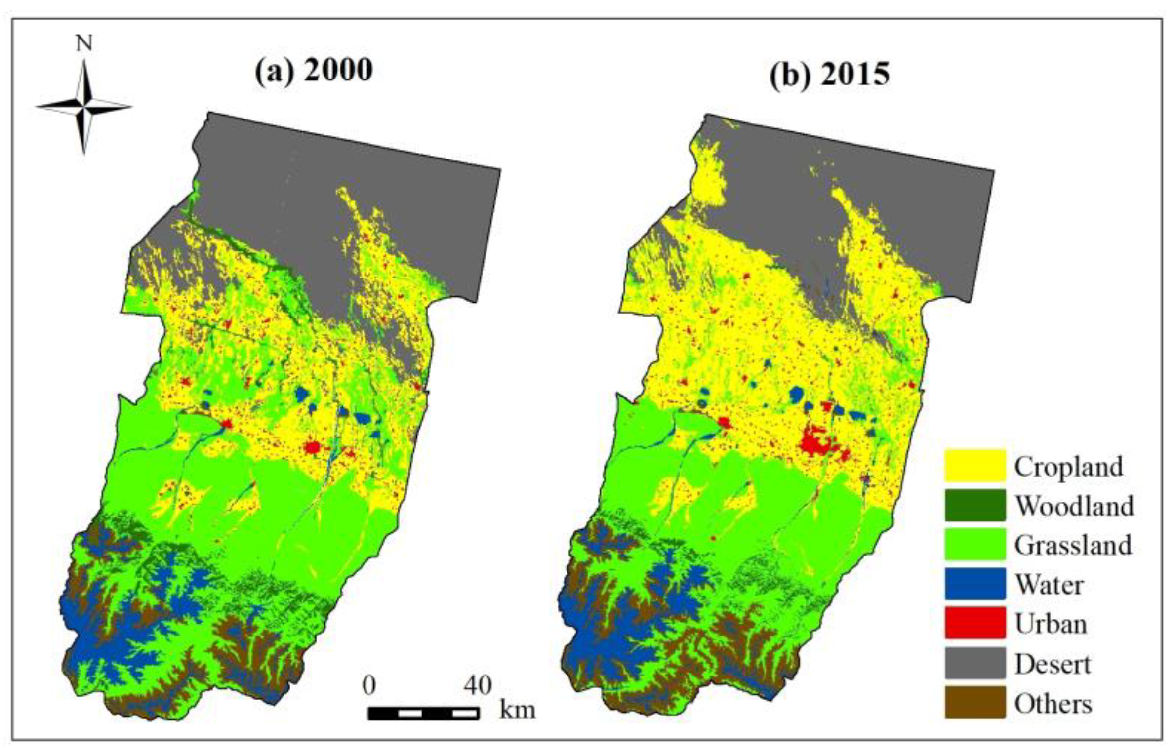
3.1. Land Use Change
3.2. Changes in Ecosystem Services Supply
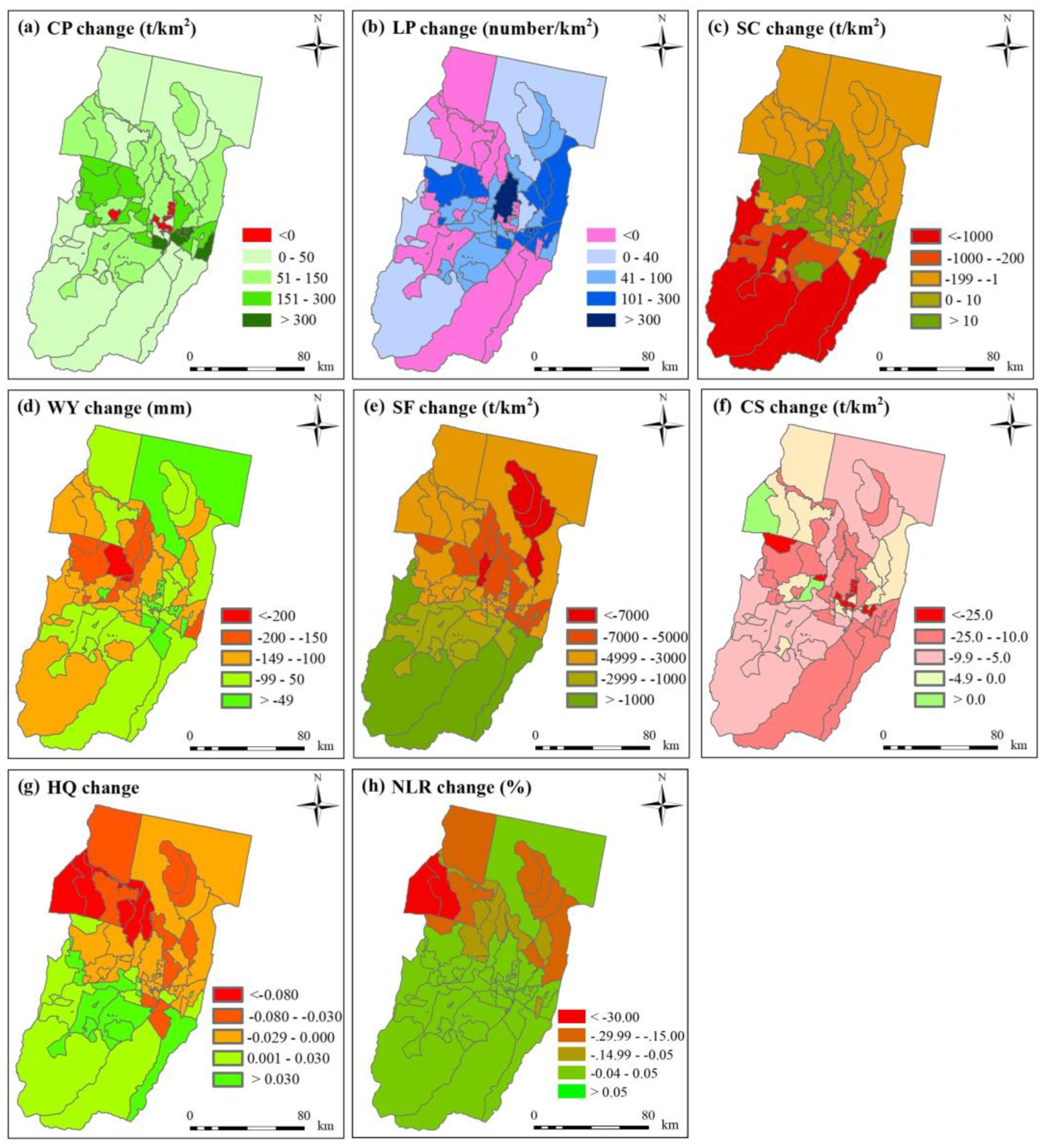
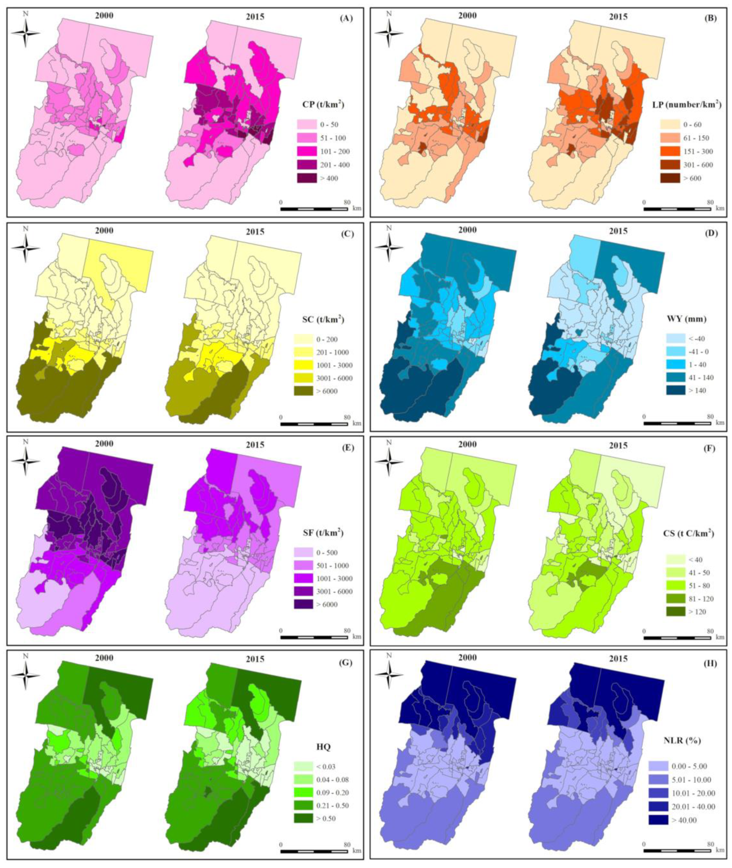
3.2.1. Spatiotemporal Changes of Individual Ecosystem Services
3.2.2. Changes in Ecosystem Service Bundles
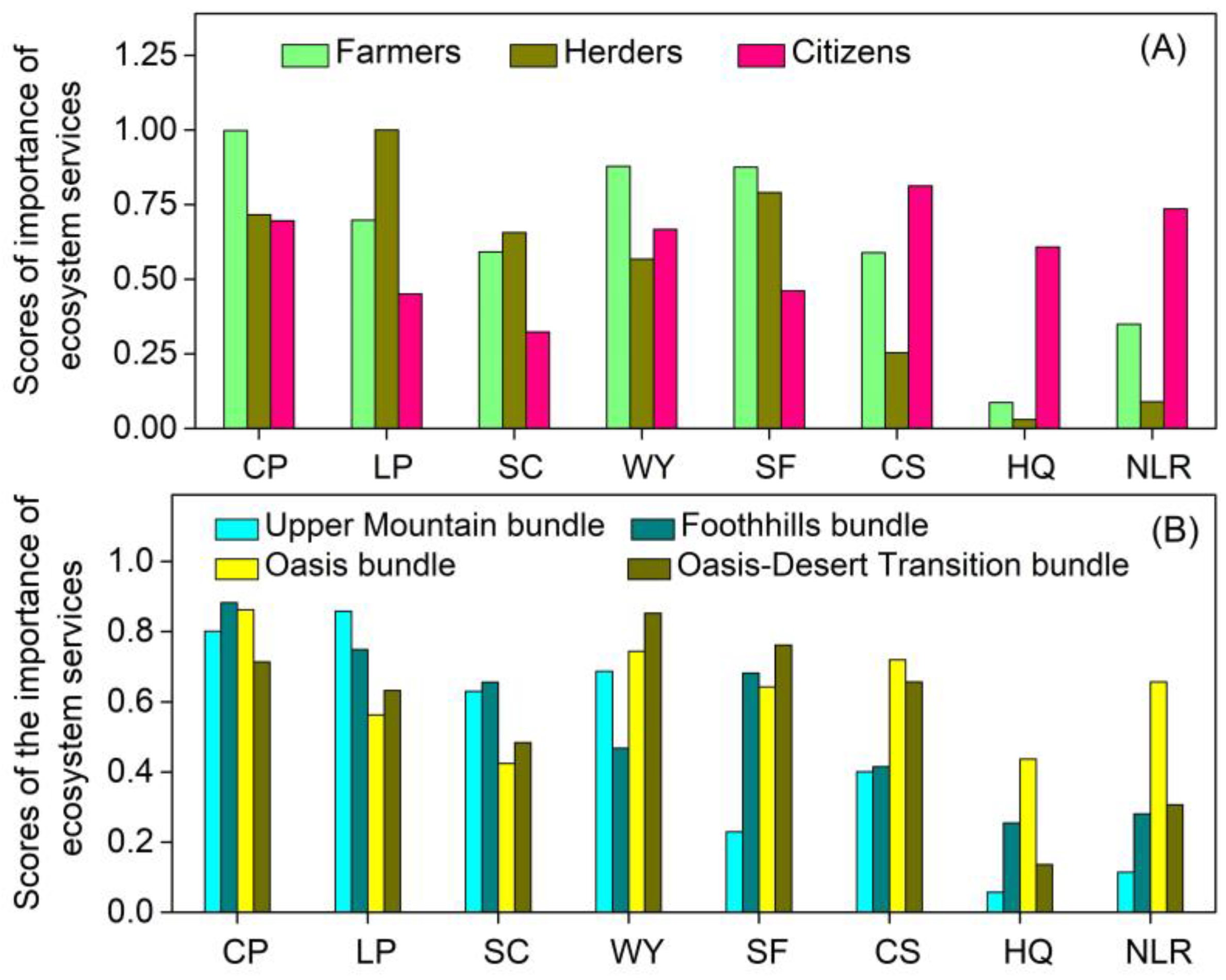
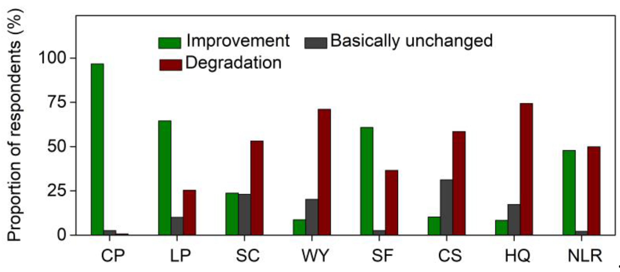
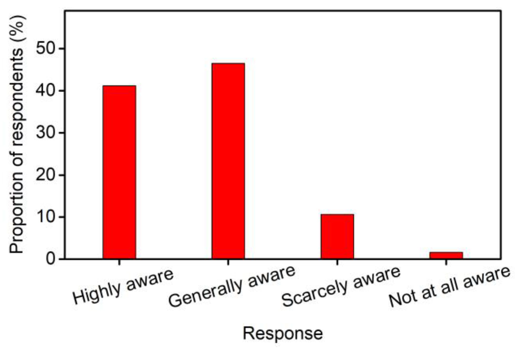
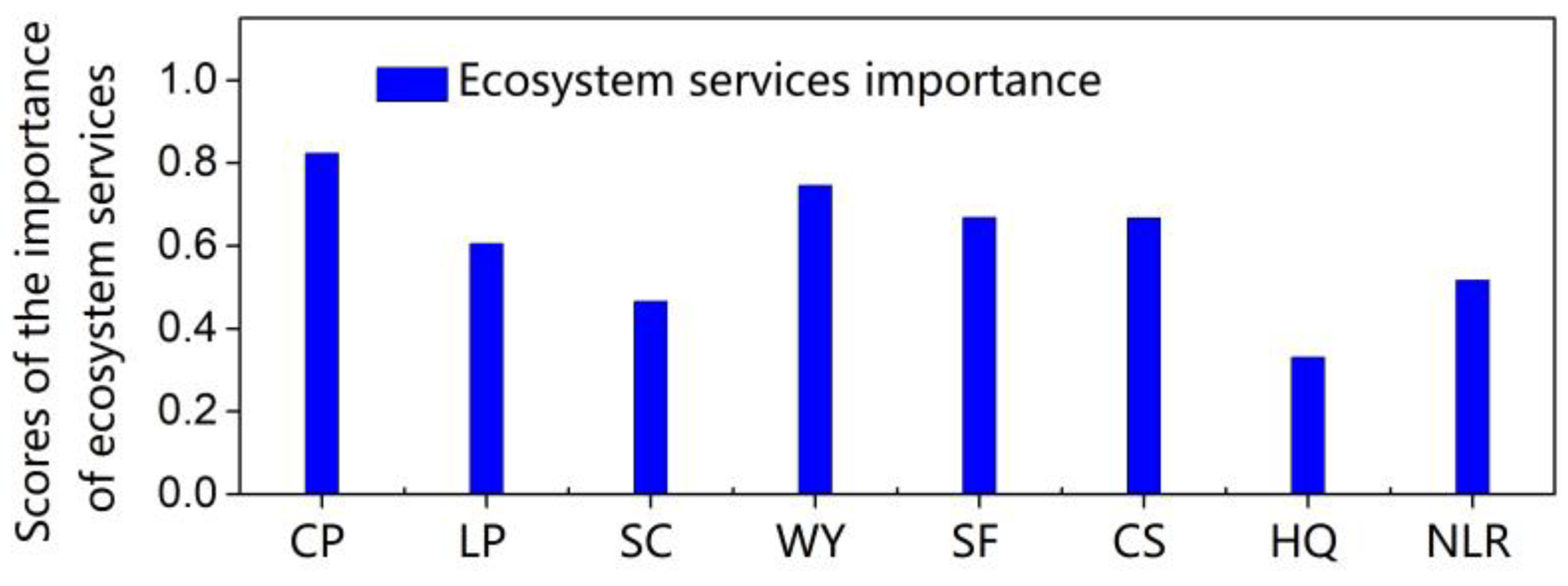
3.3. Perceptions of Ecosystem Services and Land Use Change
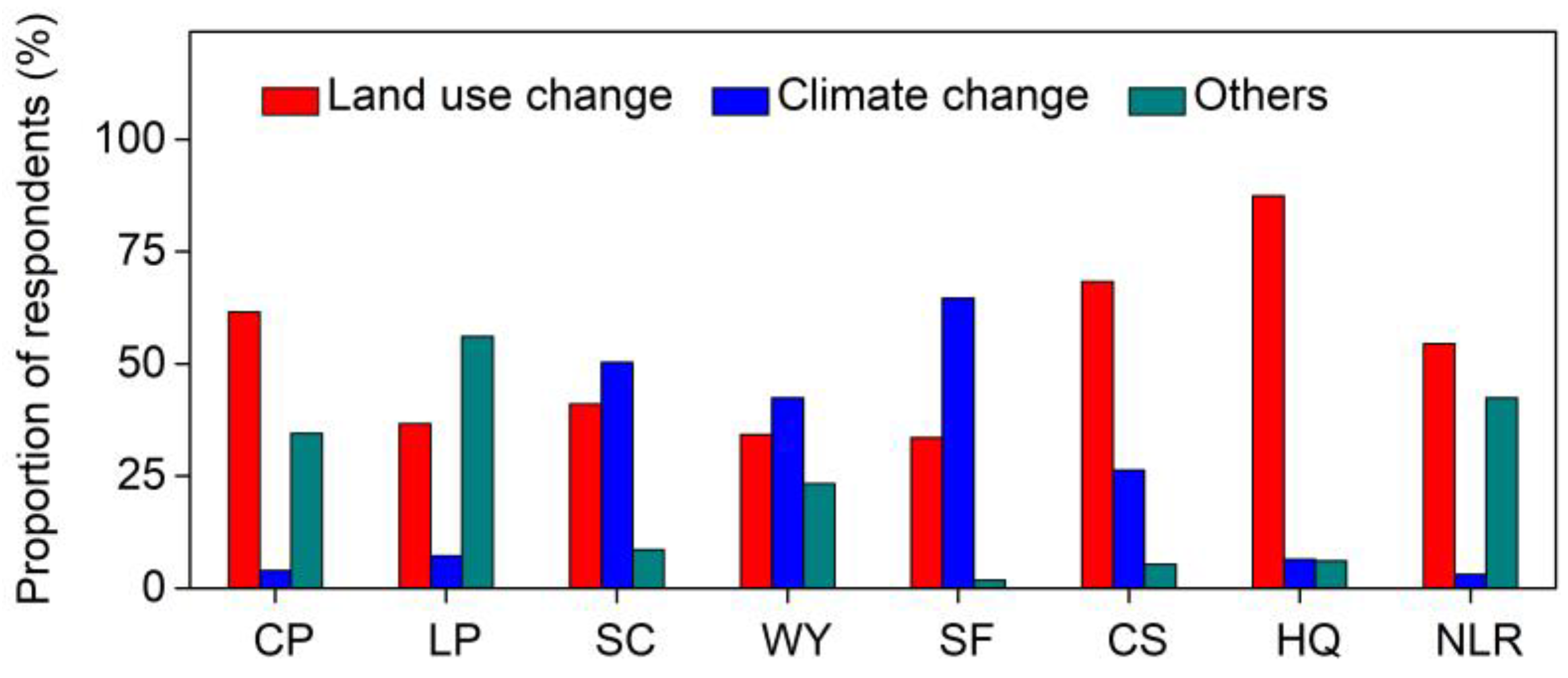
3.4. Impact of Land Use Change on Ecosystem Services
4. Discussion
4.1. Integrating Biophysical and Sociocultural Methods into Ecosystem Services and Land Use Change Research
4.2. Methodological Concerns
4.3. Policy Implications
5. Conclusions
Supplementary Materials
Author Contributions
Funding
Conflicts of Interest
Appendix A


| Land use Types | Habitat Suitability | Threatening Factors | ||||
|---|---|---|---|---|---|---|
| Settlement | Cultivation | Population | River | Road | ||
| Cropland | 0.2 | 0.7 | 0 | 0.2 | 0.1 | 0.5 |
| Woodland | 1 | 0.4 | 0.1 | 0.2 | 0.2 | 0.3 |
| Grassland | 0.6 | 0.2 | 0.5 | 0.4 | 0.1 | 0.3 |
| Water | 0.5 | 0 | 0.1 | 0.2 | 0 | 0.5 |
| Desert | 0.6 | 0.1 | 0.5 | 0.2 | 0.2 | 0.7 |
| Others | 0.1 | 0.4 | 0.1 | 0.2 | 0.2 | 0.3 |
| Characteristics | Category/Number (Proportion) |
|---|---|
| Sex | Male/462 (56.69%); Female/353 (43.31%) |
| Age | <20 years/26 (3.19%); 20–39 years/254 (31.17%); 40–59 years/505 (61.96%); ≥60 years/30 (3.68%) |
| Education | None/10 (1.23%); Primary/272 (33.37%); Secondary/269 (33.01%); University/264 (32.39%) |
| Residency period | <5 years/11 (1.35%); 5–9 years/57 (6.99%); 10–19 years/54 (6.63%); 20–39 years/354 (43.44%); ≥40 years/339 (41.60%) |
| Occupation | Farming/347 (42.58%); Grazing/69 (8.47%); Enterprise or public institution/312 (38.28); Others/87 (10.67%) |
| Land Use Types | Croplands | Woodlands | Grasslands | Urban | Water | Desert | Others |
|---|---|---|---|---|---|---|---|
| 2000 | 44.07 | 9.45 | 79.57 | 3.17 | 14.88 | 53.33 | 25.34 |
| 2015 | 53.12 | 8.77 | 75.5 | 3.77 | 14.82 | 50.69 | 23.14 |
| 2000–2015 | 9.05 | −0.68 | −4.07 | 0.60 | −0.06 | −2.64 | −2.20 |
| Proportion of the total area (%) * | 3.94 | −0.30 | −1.77 | 0.26 | −0.03 | −1.15 | −0.96 |
References
- Daily, G.C. Nature’s Services Societal Dependence on Natural Ecosystems; Island Press: Washington, DC, USA, 1997. [Google Scholar]
- Fu, B.; Zhou, G.; Bai, Y.; Song, C.; Liu, J.; Zhang, H.; Lü, Y.; Zheng, H.; Xie, G. The main terrestrial ecosystem services and ecological security in China. Adv. Earth Sci. 2009, 24, 571–576. [Google Scholar]
- Millenium Ecosystem Assessment (MEA). Ecosystem and Human Wellbeing: Current State and Trends; Island Press: Washington, DC, USA, 2005. [Google Scholar]
- Sandker, M.; Finegold, Y.; Min, Z. Forest ecology and management projecting global forest area towards 2030. For. Ecol. Manag. 2015, 52, 124–133. [Google Scholar]
- Foley, J.A.; Defries, R.; Asner, G.P.; Barford, C.; Bonan, G.; Carpenter, S.R.; Chapin, F.S.; Coe, M.T.; Daily, G.C.; Gibbs, H.K. Global consequences of land use. Science 2005, 309, 570–574. [Google Scholar] [CrossRef]
- Fu, B.; Zhang, L.; Xu, Z.; Zhao, Y.; Wei, Y.; Skinner, D. Ecosystem services in changing land use. J. Soils Sediments 2015, 15, 833–843. [Google Scholar] [CrossRef]
- Wu, X.; Wang, S.; Fu, B.; Liu, Y.; Zhu, Y. Land use optimization based on ecosystem service assessment: A case study in the Yanhe watershed. Land Use Policy 2018, 72, 303–312. [Google Scholar] [CrossRef]
- Lawler, J.J.; Lewis, D.J.; Nelson, E.; Plantinga, A.J.; Polasky, S. Projected land-use change impacts on ecosystem services in the United States. Proc. Natl. Acad. Sci. USA 2014, 201405557. [Google Scholar] [CrossRef] [PubMed]
- Metzger, M.J.; Rounsevell, M.D.A.; Acosta-Michlik, L.; Leemans, R.; Schröter, D. The vulnerability of ecosystem services to land use change. Agric. Ecosyst. Environ. 2006, 114, 69–85. [Google Scholar] [CrossRef]
- Wei, H.; Xu, Z.; Liu, H.; Ren, J.; Fan, W.; Lu, N.; Dong, X. Evaluation on dynamic change and interrelations of ecosystem services in a typical mountain-oasis-desert region. Ecol. Indic. 2018, 93, 917–929. [Google Scholar] [CrossRef]
- Kong, L.; Zheng, H.; Rao, E.; Xiao, Y.; Ouyang, Z.; Li, C. Evaluating indirect and direct effects of eco-restoration policy on soil conservation service in Yangtze River Basin. Sci. Total Environ. 2018, 631–632, 887–894. [Google Scholar] [CrossRef]
- Kremen, C.; Williams, N.M.; Aizen, M.A.; Gemmill-Herren, B.; LeBuhn, G.; Minckley, R.; Packer, L.; Potts, S.G.; Roulston, T.A.; Steffan-Dewenter, I.; et al. Pollination and other ecosystem services produced by mobile organisms: A conceptual framework for the effects of land-use change. Ecol. Lett. 2007, 10, 299–314. [Google Scholar] [CrossRef] [PubMed]
- Ray, D.K.; Duckles, J.M.; Pijanowski, B.C. The impact of future land use scenarios on runoff volumes in the Muskegon River watershed. Environ. Manag. 2010, 46, 351–366. [Google Scholar] [CrossRef]
- Sherrouse, B.C.; Semmens, D.J.; Ancona, Z.H.; Brunner, N.M. Analyzing land-use change scenarios for trade-offs among cultural ecosystem services in the Southern Rocky Mountains. Ecosyst. Serv. 2017, 26, 431–444. [Google Scholar] [CrossRef]
- Stockmann, U.; Adams, M.A.; Crawford, J.W.; Zimmermann, M. The knowns, known unknowns and unknowns of sequestration of soil organic carbon. Agric. Ecosyst. Environ. 2015, 164, 80–99. [Google Scholar] [CrossRef]
- Arowolo, A.O.; Deng, X.; Olatunji, O.A.; Obayelu, A.E. Assessing changes in the value of ecosystem services in response to land-use/land-cover dynamics in Nigeria. Sci. Total Environ. 2018, 636, 597–609. [Google Scholar] [CrossRef]
- Costanza, R.; de Groot, R.; Sutton, P.; van der Ploeg, S.; Anderson, S.J.; Kubiszewski, I.; Farber, S.; Turner, R.K. Changes in the global value of ecosystem services. Glob. Environ. Chang. 2014, 26, 152–158. [Google Scholar] [CrossRef]
- Gong, J.; Li, J.; Yang, J.; Li, S.; Tang, W. Land Use and Land Cover Change in the Qinghai Lake Region of the Tibetan Plateau and Its Impact on Ecosystem Services. Int. J. Environ. Res. Public Health 2017, 14, 818. [Google Scholar] [CrossRef] [PubMed]
- Mendoza-González, G.; Martínez, M.L.; Lithgow, D.; Pérez-Maqueo, O.; Simonin, P. Land use change and its effects on the value of ecosystem services along the coast of the Gulf of Mexico. Ecol. Econ. 2012, 82, 23–32. [Google Scholar] [CrossRef]
- Zhou, D.; Tian, Y.; Jiang, G. Spatio-temporal investigation of the interactive relationship between urbanization and ecosystem services: Case study of the Jingjinji urban agglomeration, China. Ecol. Indic. 2018, 95, 152–164. [Google Scholar] [CrossRef]
- Allan, E.; Manning, P.; Alt, F.; Binkenstein, J.; Blaser, S.; Blüthgen, N.; Kleinebecker, T. Land use intensification alters ecosystem multifunctionality via loss of biodiversity and changes to functional composition. Ecol. Lett. 2015, 18, 834–843. [Google Scholar] [CrossRef] [PubMed] [Green Version]
- Laliberté, E.; Tylianakis, J.M. Cascading effects of long-term land-use changes on plant traits and ecosystem functioning. Ecology 2012, 93, 145–155. [Google Scholar] [CrossRef] [PubMed]
- Martínez, M.L.; Pérez-Maqueo, O.; Vázquez, G.; Castillo-Campos, G.; García-Franco, J.; Mehltreter, K.; Equihua, M.; Landgrave, R. Effects of land use change on biodiversity and ecosystem services in tropical montane cloud forests of Mexico. For. Ecol. Manag. 2009, 258, 1856–1863. [Google Scholar] [CrossRef]
- Impact of land-use change on biodiversity and ecosystem services in the Chilean temperate forests. Landsc. Ecol. 2018, 33, 439–453. [CrossRef]
- Yi, H.; Guneralp, B.; Kreuter, U.P.; Guneralp, I.; Filippi, A.M. Spatial and temporal changes in biodiversity and ecosystem services in the San Antonio River Basin, Texas, from 1984 to 2010. Sci. Total Environ. 2018, 619–620, 1259–1271. [Google Scholar] [CrossRef] [PubMed]
- Fu, Q.; Li, B.; Hou, Y.; Bi, X.; Zhang, X. Effects of land use and climate change on ecosystem services in Central Asia’s arid regions: A case study in Altay Prefecture, China. Sci. Total Environ. 2017, 607–608, 633–646. [Google Scholar] [CrossRef]
- Sun, X.; Crittenden, J.C.; Li, F.; Lu, Z.; Dou, X. Urban expansion simulation and the spatio-temporal changes of ecosystem services, a case study in Atlanta Metropolitan area, USA. Sci. Total Environ. 2018, 622–623, 974–987. [Google Scholar] [CrossRef] [PubMed]
- Wei, H.; Fan, W.; Ding, Z.; Weng, B.; Xing, K.; Wang, X.; Lu, N.; Ulgiati, S.; Dong, X. Ecosystem Services and Ecological Restoration in the Northern Shaanxi Loess Plateau, China, in Relation to Climate Fluctuation and Investments in Natural Capital. Sustainability 2017, 9, 199. [Google Scholar] [CrossRef]
- Xie, W.; Huang, Q.; He, C.; Zhao, X. Projecting the impacts of urban expansion on simultaneous losses of ecosystem services: A case study in Beijing, China. Ecol. Indic. 2018, 84, 183–193. [Google Scholar] [CrossRef]
- Kong, L.; Zheng, H.; Xiao, Y.; Ouyang, Z.; Li, C.; Zhang, J.; Huang, B. Mapping Ecosystem Service Bundles to Detect Distinct Types of Multifunctionality within the Diverse Landscape of the Yangtze River Basin, China. Sustainability 2018, 10, 857. [Google Scholar] [CrossRef]
- Zhao, M.; Peng, J.; Liu, Y.; Li, T.; Wang, Y. Mapping Watershed-Level Ecosystem Service Bundles in the Pearl River Delta, China. Ecol. Econ. 2018, 152, 106–117. [Google Scholar] [CrossRef]
- Saidi, N.; Spray, C. Ecosystem services bundles: Challenges and opportunities for implementation and further research. Environ. Res. Lett. 2018, 13, 113001. [Google Scholar] [CrossRef]
- Raudsepp-Hearne, C.; Peterson, G.D.; Bennett, E.M. Ecosystem service bundles for analyzing tradeoffs in diverse landscapes. Proc. Natl. Acad. Sci. USA 2010, 107, 5242–5247. [Google Scholar] [CrossRef] [PubMed] [Green Version]
- Baró, F.; Gómez-Baggethun, E.; Haase, D. Ecosystem service bundles along the urban-rural gradient: Insights for landscape planning and management. Ecosyst. Serv. 2017, 24, 147–159. [Google Scholar] [CrossRef]
- Martín-López, B.; Iniesta-Arandia, I.; García-Llorente, M.; Palomo, I.; Casado-Arzuaga, I.; Del Amo, D.G.; Gómez-Baggethun, E.; Oteros-Rozas, E.; Palacios-Agundez, I.; Willaarts, B.; et al. Uncovering ecosystem service bundles through social preferences. PLoS ONE 2012, 7, e38970. [Google Scholar] [CrossRef] [PubMed]
- Schirpke, U.; Candiago, S.; Egarter Vigl, L.; Jager, H.; Labadini, A.; Marsoner, T.; Meisch, C.; Tasser, E.; Tappeiner, U. Integrating supply, flow and demand to enhance the understanding of interactions among multiple ecosystem services. Sci. Total Environ. 2019, 651 Pt 1, 928–941. [Google Scholar] [CrossRef]
- Yang, G.; Ge, Y.; Xue, H.; Yang, W.; Shi, Y.; Peng, C.; Du, Y.; Fan, X.; Ren, Y.; Chang, J. Using ecosystem service bundles to detect trade-offs and synergies across urban–rural complexes. Landsc. Urban Plan. 2015, 136, 110–121. [Google Scholar] [CrossRef]
- Shoyama, K.; Yamagata, Y. Local perception of ecosystem service bundles in the Kushiro watershed, Northern Japan—Application of a public participation GIS tool. Ecosyst. Serv. 2016, 22, 139–149. [Google Scholar] [CrossRef]
- Yao, J.; He, X.; Chen, W.; Ye, Y.; Guo, R.; Yu, L. A local-scale spatial analysis of ecosystem services and ecosystem service bundles in the upper Hun River catchment, China. Ecosyst. Serv. 2016, 22, 104–110. [Google Scholar] [CrossRef]
- Dittrich, A.; Seppelt, R.; Václavík, T.; Cord, A.F. Integrating ecosystem service bundles and socio-environmental conditions—A national scale analysis from Germany. Ecosyst. Serv. 2017, 28, 273–282. [Google Scholar] [CrossRef]
- Hamann, M.; Biggs, R.; Reyers, B. Mapping social–ecological systems: Identifying ‘green-loop’ and ‘red-loop’ dynamics based on characteristic bundles of ecosystem service use. Glob. Environ. Chang. 2015, 34, 218–226. [Google Scholar] [CrossRef] [Green Version]
- Mouchet, M.A.; Paracchini, M.L.; Schulp, C.J.E.; Stürck, J.; Verkerk, P.J.; Verburg, P.H.; Lavorel, S. Bundles of ecosystem (dis)services and multifunctionality across European landscapes. Ecol. Indic. 2017, 73, 23–28. [Google Scholar] [CrossRef]
- Wei, H.J.; Liu, H.M.; Xu, Z.H.; Ren, J.H.; Lu, N.C.; Fan, W.G.; Zhang, P.; Dong, X.B. Linking ecosystem services supply, social demand and human well-being in a typical mountain–oasis–desert area, Xinjiang, China. Ecosyst. Serv. 2018, 31, 44–57. [Google Scholar] [CrossRef]
- Gaglio, M.; Aschonitis, V.G.; Gissi, E.; Castaldelli, G.; Fano, E.A. Land use change effects on ecosystem services of river deltas and coastal wetlands: Case study in Volano–Mesola–Goro in Po river delta (Italy). Wetl. Ecol. Manag. 2016, 25, 67–86. [Google Scholar] [CrossRef]
- Zorrilla-Miras, P.; Palomo, I.; Gómez-Baggethun, E.; Martín-López, B.; Lomas, P.L.; Montes, C. Effects of land-use change on wetland ecosystem services: A case study in the Doñana marshes (SW Spain). Landsc. Urban Plan. 2014, 122, 160–174. [Google Scholar] [CrossRef]
- Rukundo, E.; Liu, S.; Dong, Y.; Rutebuka, E.; Asamoah, E.F.; Xu, J.; Wu, X. Spatio-temporal dynamics of critical ecosystem services in response to agricultural expansion in Rwanda, East Africa. Ecol. Indic. 2018, 89, 696–705. [Google Scholar] [CrossRef]
- Gong, L.; Ran, Q.; He, G.; Tiyip, T. A soil quality assessment under different land use types in Keriya river basin, Southern Xinjiang, China. Soil Tillage Res. 2015, 146, 223–229. [Google Scholar] [CrossRef]
- Cheng, W.; Zhou, C.; Liu, H.; Zhang, Y.; Jiang, Y.; Zhang, Y.; Yao, Y. The oasis expansion and eco-environment change over the last 50 years in Manas River Valley, Xinjiang. Sci. China Ser. D 2006, 49, 163–175. [Google Scholar] [CrossRef]
- Zhang, H.; Ouyang, Z.; Zheng, H.; Xiao, Y. Valuation of glacier ecosystem services in the Manas River Watershed, Xinjiang. Acta Ecol. Sin. 2009, 29, 5877–5881. (In Chinese) [Google Scholar]
- Zhang, H.; Ouyang, Z.; Zheng, H.; Xiao, Y. Evaluation of agricultural ecosystem services value in Manas River Watershed of China. Chin. J. Eco-Agric. 2009, 17, 1259–1264. (In Chinese) [Google Scholar] [CrossRef]
- Millennium Ecosystem Assessment. Ecosystems and Human Well-Being Synthesis; Island Press: Washington, DC, USA, 2014. [Google Scholar]
- Xinjiang Uygur Autonomous Region Bureau of Statistics. Xinjiang Uygur Autonomous Region Statistical Yearbook; China Statistical Publishing House: Beijing, China, 2001 and 2016. (In Chinese) [Google Scholar]
- National Climatic Bureau in China. Available online: http://data.cma.cn (accessed on 10 January 2018).
- Chinese Academy of Sciences. Available online: http://www.resdc.cn (accessed on 10 January 2018).
- National Aeronautics and Space Administration. Available online: https://lpdaac.usgs.gov/ (accessed on 10 January 2018).
- National Natural Science Foundation of China. Available online: http://westdc.westgis.ac.cn (accessed on 10 January 2018).
- Renard, K.G.; Foster, G.R.; Weesies, G.A.; Porter, J.P. RUSLE: Revised universal soil loss equation. J. Soil Water Conserv. 1991, 46, 30–33. [Google Scholar]
- Budyko, M.I. Climate and Life; Academic Press: New York, NY, USA, 1974. [Google Scholar]
- Fryrear, D.W.; Bilbro, J.D.; Saleh, A.; Schomberg, H.; Stout, J.E.; Zobeck, T.M. RWEQ: Improved wind erosion technology. J. Soil Water Conserv. 2000, 55, 183–189. [Google Scholar]
- Field, C.B.; Randerson, J.T.; Malmström, C.M. Global net primary production: Combining ecology and remote sensing. Remote Sens. Environ. 1995, 51, 74–88. [Google Scholar] [CrossRef] [Green Version]
- Tallis, H.T.; Ricketts, T.; Guerry, A.D.; Wood, S.A.; Sharp, R.; Nelson, E.; Ennaanay, D.; Wolny, S.; Olwero, N.; Vigerstol, K.; et al. InVEST 2.5.3 User’s Guide; The Natural Capital Project: Stanford, CA, USA, 2013. [Google Scholar]
- Wischmeier, W.H.; Johnson, C.B.; Cross, B.V. Soil erodibility nomograph for farmland and construction sites. J. Soil Water Conserv. 1971, 26, 189–193. [Google Scholar]
- Sharpley, A.N.; Williams, J.R. EPIC-erosion/productivity impact calculator: 1. model documentation. USDA Tech. Bull. 1990, 4, 206–207. [Google Scholar]
- McCool, D.K.; Brown, L.C.; Foster, G.R.; Mutchler, C.K.; Meyer, L.D. Revised slope steepness factor for the Universal Soil Loss Equation. Trans. ASAE 1987, 30, 1387–1396. [Google Scholar] [CrossRef]
- McCool, D.K.; Foster, G.R.; Mutchler, C.K.; Meyer, L.D. Revised slope length factor for the Universal Soil Loss Equation. Trans. ASAE 1989, 32, 1571–1576. [Google Scholar] [CrossRef]
- Lufafa, A.; Tenywa, M.M.; Isabirye, M.; Majaliwa, M.J.G.; Woomer, P.L. Prediction of soil erosion in a Lake Victoria basin catchment using a GIS-based Universal Soil Loss model. Agric. Syst. 2003, 76, 883–894. [Google Scholar] [CrossRef]
- Sun, G.; Alstad, K.; Chen, J.; Chen, S.; Ford, C.R.; Lin, G.; Noormets, A. A general predictive model for estimating monthly ecosystem evapotranspiration. Ecohydrology 2011, 4, 245–255. [Google Scholar] [CrossRef]
- Samani, Z.A.; Pessarakli, M. Estimating potential crop evapotranspiration with minimum data in Arizona. Trans. ASAE 1986, 29, 522–0524. [Google Scholar] [CrossRef]
- Ouyang, Z.; Zheng, H.; Xiao, Y.; Polasky, S.; Liu, J.; Xu, W.; Wang, Q.; Zhang, L.; Xiao, Y.; Rao, E.; et al. Improvements in ecosystem services from investments in natural capital. Science 2016, 352, 1455–1459. [Google Scholar] [CrossRef]
- Potter, C.S.; Randerson, J.T.; Field, C.B.; Matson, P.A.; Vitousek, P.M.; Mooney, H.A.; Klooster, S.A. Terrestrial ecosystem production: A process model based on global satellite and surface data. Glob. Biogeochem. Cycles 1993, 7, 811–841. [Google Scholar] [CrossRef]
- Zhu, W.Q.; Pan, Y.Z.; He, H.; Yu, D.Y.; Hu, H.B. Simulation of maximum light use efficiency for some typical vegetation types in China. Chin. Sci. Bull. 2006, 51, 457–463. [Google Scholar] [CrossRef]
- Depellegrin, D.; Pereira, P.; Misiunė, I.; Egarter-Vigl, L. Mapping ecosystem services potential in Lithuania. Int. J. Sustain. Dev. World Ecol. 2016, 23, 441–455. [Google Scholar] [CrossRef]
- Marsboom, C.; Vrebos, D.; Staes, J.; Meire, P. Using dimension reduction PCA to identify ecosystem service bundles. Ecol. Indic. 2018, 87, 209–260. [Google Scholar] [CrossRef]
- Crouzat, E.; Mouchet, M.; Turkelboom, F.; Byczek, C.; Meersmans, J.; Berger, F.; Verkerk, P.J.; Lavorel, S. Assessing bundles of ecosystem services from regional to landscape scale: Insights from the French Alps. J. Appl. Ecol. 2015, 52, 1145–1155. [Google Scholar] [CrossRef]
- Lamy, T.; Liss, K.N.; Gonzalez, A.; Bennett, E.M. Landscape structure affects the provision of multiple ecosystem services. Environ. Res. Lett. 2016, 11, 124017. [Google Scholar] [CrossRef] [Green Version]
- Wei, H.; Fan, W.; Wang, X.; Lu, N.; Dong, X.; Zhao, Y.; Ya, X.; Zhao, Y. Integrating supply and social demand in ecosystem services assessment: A review. Ecosyst. Serv. 2017, 25, 15–27. [Google Scholar] [CrossRef]
- Compton, J.E.; Harrison, J.A.; Dennis, R.L.; Greaver, T.L.; Hill, B.H.; Jordan, S.J.; Walker, H.; Campbell, H.V. Ecosystem services altered by human changes in the nitrogen cycle: A new perspective for US decision making. Ecol. Lett. 2011, 14, 804–815. [Google Scholar] [CrossRef]
- Burkhard, B.; Kroll, F.; Nedkov, S.; Müller, F. Mapping ecosystem service supply, demand and budgets. Ecol. Indic. 2012, 21, 17–29. [Google Scholar] [CrossRef]
- Wu, X.; Liu, S.; Zhao, S.; Hou, X.; Xu, J.; Dong, S.; Liu, G. Quantification and driving force analysis of ecosystem services supply, demand and balance in China. Sci. Total Environ. 2019, 652, 1375–1386. [Google Scholar] [CrossRef]
- Li, T.; Li, J.; Wang, Y. Carbon sequestration service flow in the Guanzhong-Tianshui economic region of China: How it flows, what drives it, and where could be optimized? Ecol. Indic. 2019, 96, 548–558. [Google Scholar] [CrossRef]
- Zhao, Q.; Li, J.; Liu, J.; Cuan, Y.; Zhang, C. Integrating supply and demand in cultural ecosystem services assessment: A case study of Cuihua Mountain (China). Environ. Sci. Pollut. Res. 2019, 26, 6065–6076. [Google Scholar] [CrossRef] [PubMed]
- Rodríguez, J.; Beard, T.; Bennett, E.; Cumming, G.; Cork, S.; Agard, J.; Dobson, A.; Peterson, G. Trade-offs across space, time, and ecosystem services. Ecol. Soc. 2006, 11, 28. [Google Scholar] [CrossRef]


| Data Types | Data Contents | Data Purposes | Data Sources |
|---|---|---|---|
| Statistical data | Crop production and livestock inventory | Evaluating CP and LP | Statistical yearbooks [52] |
| Meteorological and hydrological data | Daily solar radiation, temperature, precipitation, and wind speed | Input parameters of SC, WY, SF, and CS evaluation | National Climatic Bureau [53] |
| Annual runoffs | Evaluating rationality of WY change | ||
| Land use data | Cropland, woodland, grassland, water, urban, and desert | Evaluating land use change and NLR; Input parameters of SC, SF, CS, and HQ evaluation | Data Center for Resources and Environmental Sciences, Chinese Academy of Sciences [54] |
| Basic geographic data | Road network and water system | Input parameters of HQ evaluation | |
| Elevation | Input parameters of SC evaluation | ||
| Remote sensing data | MOD13 NDVI and MOD15 LAI | Input parameters of SC, WY, SF, and CS evaluation | NASA’s Earth data [55] |
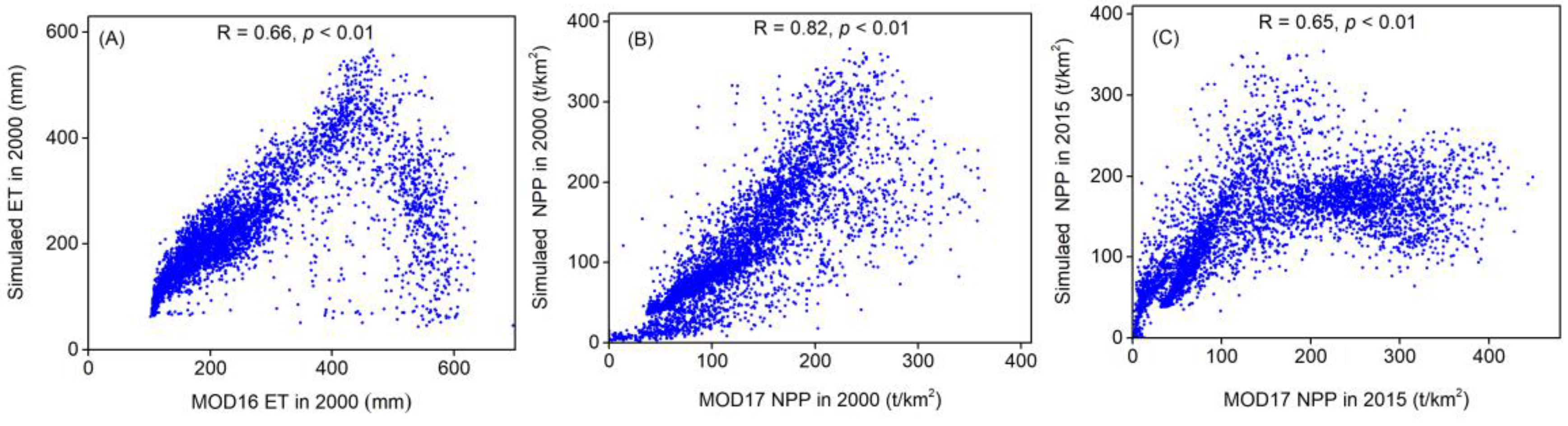
| MOD16 ET and MOD17 NPP | Verification of estimation accuracy of ET and NPP | ||
| Soil attribute data | Content of sand, silt, clay, and organic carbon | Input parameters of SC and SF evaluation | Cold and Arid Regions Sciences Data Center at Lanzhou [56] |
| Ecosystem Services (ESs) | Indicators | Units | Approaches |
|---|---|---|---|
| Provisioning | |||
| Crop production (CP) | Annual crop output | t/km2 | Statistical data in township-level units |
| Livestock Production (LP) | Livestock inventory | number/km2 | Statistical data in township-level units |
| Regulating | |||
| Soil conservation (SC) | Soil retention amount | t/km2 | Revised universal soil loss equation (RUSLE) [57] |
| Water yield (WY) | Water output | mm | Water balance equation [58] |
| Sand fixation (SF) | Binding sand quantity | t/km2 | Revised wind erosion equation (RWEQ) [59] |
| Carbon sequestration (CS) | Carbon sequestration of noncrop plants [33] | t/km2 | Carnegie Ames Stanford Approach (CASA) [60] |
| Habitat quality (HQ) | Habitat quality index | Dimensionless index (0–1) | InVEST (Integrate valuation of ES and tradeoffs) habitat quality model [61] |
| Cultural | |||
| Nature landscape recreation * (NLR) | Proportion of forest and desert cover | % | Remote sensing interpretation (Landsat) |
| ES | CP | LP | SC | WY | SF | CS | HQ | NLR |
|---|---|---|---|---|---|---|---|---|
| R1 | 0.504 ** | 0.119 | 0.190 | −0.679 ** | −0.255 | −0.537 ** | −0.432 ** | −0.526 ** |
| R2 | −0.149 | 0.245 | 0.157 | 0.349 * | −0.144 | −0.231 | 0.021 | 0.017 |
| PR1 | 0.428 ** | −0.048 | 0.008 | −0.643 ** | −0.189 | −0.711 ** | −0.439 ** | −0.545 ** |
| PR2 | −0.235 | −0.042 | −0.050 | 0.271 * | −0.066 | −0.430 ** | −0.089 | −0.133 |
© 2019 by the authors. Licensee MDPI, Basel, Switzerland. This article is an open access article distributed under the terms and conditions of the Creative Commons Attribution (CC BY) license (http://creativecommons.org/licenses/by/4.0/).
Share and Cite
Wei, H.; Fan, W.; Lu, N.; Xu, Z.; Liu, H.; Chen, W.; Ulgiati, S.; Wang, X.; Dong, X. Integrating Biophysical and Sociocultural Methods for Identifying the Relationships between Ecosystem Services and Land Use Change: Insights from an Oasis Area. Sustainability 2019, 11, 2598. https://0-doi-org.brum.beds.ac.uk/10.3390/su11092598
Wei H, Fan W, Lu N, Xu Z, Liu H, Chen W, Ulgiati S, Wang X, Dong X. Integrating Biophysical and Sociocultural Methods for Identifying the Relationships between Ecosystem Services and Land Use Change: Insights from an Oasis Area. Sustainability. 2019; 11(9):2598. https://0-doi-org.brum.beds.ac.uk/10.3390/su11092598
Chicago/Turabian StyleWei, Hejie, Weiguo Fan, Nachuan Lu, Zihan Xu, Huiming Liu, Weiqiang Chen, Sergio Ulgiati, Xuechao Wang, and Xiaobin Dong. 2019. "Integrating Biophysical and Sociocultural Methods for Identifying the Relationships between Ecosystem Services and Land Use Change: Insights from an Oasis Area" Sustainability 11, no. 9: 2598. https://0-doi-org.brum.beds.ac.uk/10.3390/su11092598