Do Larger Cities Experience Lower Crime Rates? A Scaling Analysis of 758 Cities in the U.S.

1
Gachon Center for Convergence Research, Gachon University, 1342 Seongnam-daero, Sujung-gu, Gyeonggi-do 13120, Korea
2
Department of Global Business, Gachon University, 1342 Seongnam-daero, Sujung-gu, Gyeonggi-do 13120, Korea
*
Author to whom correspondence should be addressed.
Sustainability 2019, 11(11), 3111; https://0-doi-org.brum.beds.ac.uk/10.3390/su11113111
Submission received: 22 April 2019
/
Revised: 26 May 2019
/
Accepted: 28 May 2019
/
Published: 2 June 2019
(This article belongs to the Section Sustainable Urban and Rural Development)
Abstract
:Do larger cities still suffer from higher crime rates? The scaling relationship between the number of crimes and the population size for the maximum of 758 cities with more than 50,000 inhabitants in the United States from 1999 to 2014 was analyzed. For the total group of cities, the relationship is superlinear for both violent and property crimes. However, for the subgroups of the top 12, top 24, and top 50 largest cities, the relationship changes to sublinear for both violent and property crimes. Results from the panel data analysis are in support of these findings. Along with population size, income per capita and population density also influence the outcome of crime counts. Implications from these findings will be discussed.
1. Introduction
What is the relationship between the crime count and population size of cities? Do larger cities always experience higher crime rates compared to smaller cities? Although larger cities have historically experienced higher crimes rates in the past [1,2], this situation may have changed in recent years so that very large cities may be experiencing lower crime rates compared to middle-sized cities [3,4]. If this new trend continues, it will have a significantly positive impact on mitigating overall crime rates in the future, because an increasingly large number of people will reside in larger cities with populations of more than one million, with lower crime rates. For example, there are 12 cities in the U.S with populations of more than one million people, ranging from New York City with 8.6 million to San Jose with 1 million residents as of 2014. As the number of cities and their residents continues to grow, they will benefit from lower crime rates in the future. Brooking’s study [5] estimated that the combination of direct monetary losses and the costs of pain and suffering among crime victims in the U.S amount to nearly 6 percent of the gross domestic product.
Therefore, the major question of this research is to determine whether the crime rate varies among subgroups of cities with different population sizes. For example, does the subgroup of the top 12 largest cities with more than one million inhabitants display lower crime rates in comparison to other subgroups of cities with smaller populations? This question will be examined for violent crime and property crime, covering between 91 and 758 cities in the U.S with more than 50,000 inhabitants from 1999 to 2014. For the methodology, we used the urban scaling model proposed by Bettencourt et al. [6]. We used yearly bivariate regression as well as multiple regression by adding two control variables of income per capita and population density. We also ran panel data analysis.
Following this introduction, this paper contains four additional sections. The second section presents the literature survey of empirical studies dealing with relationship between crime and city size. Particular emphasis is given to findings dealing with lower crime rates being experienced by subgroups of very large cities. In the third section, we develop our methods of analysis and explain the data we used. The fourth section presents results of our analysis. The final section presents conclusions and policy implications as well as the limitations of this study.
2. Literature Review
There have been a large number of empirical studies conducted in the past which show that crime rates in larger cities are significantly higher than those in smaller cities. One of the early studies using the U.S. Uniform Crime Statistics for 1971 showed that the homicide rate for cities with over 250,000 people was 1.9 per 10,000 inhabitants, which was nearly five times higher than the 0.4 found for cities with less than 10,000 inhabitants [1]. In the case of robberies, the rate was more than 20 times higher for cities with over 25,000 people at 63.3, compared with 3.1 for cities with under 10,000 inhabitants. The finding of the bigger the city, the higher the crime rate was also reported by several other earlier studies [7,8,9].
One of the most cited studies was by Gleaser and Sacerdote [2], in which they discovered an overall elasticity of 0.16 when they regressed serious crimes per capita to the population size of cities, using 1982 data from Uniform Crime Reports (UCR) published by the Federal Bureau of Investigation. Using the 1970 UCR data, the elasticity was higher at 0.28. Both results support the earlier findings that the bigger the city, the higher the crime rate.
Bettencourt et al. (2007) proposed urban scaling theory, suggesting that several undesirable social and environmental measures such as crime, infectious disease, congestion, and poverty may increase proportionately more as the population size of a city increases [10]. In other words, the relationship between crime incidence to population size of a city may be superlinear. The general quantitative relationship is defined by a simple power function of:
where Y is the crime count, P is the population size of the city, a is a constant, and i indexes the individual city. The exponent b determines the scaling relationship between Y and P. When the relationship is superlinear, b > 1; when the relationship is sublinear, b < 1; when the relationship is linear, b = 1.
Yi = aPib,
For example, the elasticity of 0.16 discovered by Gleaser and Sacerdote [2] is equivalent to a superlinear exponent b of 1.125. The result of the first empirical study generated the superlinear exponent of 1.16 [10], followed by another superlinear exponent of 1.2 from 2008 violent crime counts in Japan [11]. Another superlinear exponent of 1.2 was also reported for violent crime counts in Brazil [12]. Most recently, Bettencourt reported the superlinear exponents of eleven different types of crime counts for total, violent, and property crimes, as well as eight individual types of crimes involving 189 to 250 U.S. cities with over 100,000 inhabitants during the period of 1995 to 2010 [13]. The result was that all 176 scale exponents displayed superlinear relationships, ranging from 1.32 as the averaged exponent for violent crimes and 1.16 as the averaged exponent for property crimes.
Such conclusive evidence of the superlinear relationship of crime counts to the population size of cities can be explained by several well-known sociological theories [14,15,16,17,18,19,20,21]. However, none of these theories indicate any specific quantitative relationship between crime and the size of the city. Because of the overwhelming evidence in support of superlinear relationships between crime and city size, very few academic studies examining alternative relationships have been published so far.
However, there are some interesting new developments occurring in other related fields which are also subjected to urban scale theory. For example, in the field of traffic congestion, there now exist two schools—one advocating an urban congestion advantage [22,23,24] for large size cities versus the urban congestion penalty [25,26]. In the field of health care, there are also two schools—one advocating the urban health advantage for larger cities [13,27,28,29,30] versus the urban health penalty [25,26]. Similarly, in the field of pollution, there exist two schools—one advocating an urban pollution advantage [31,32,33,34,35,36] for large cities versus the urban pollution penalty [37,38,39].
One interesting common theme that urban scale advantage claims is that the bigger the size of the city, the less the negative impact from the measures associated with large size cities, such as disease, pollution, congestion, and crime. Another common theme is that urban advantage theory claims to reflect more recent new developments in large sized cities, so that larger cities in modern times become greener, healthier, less congested, and safer from crimes than small sized cities and rural areas.
In light of these recent developments in urban scale advantage, it may be useful to examine the question of urban crime advantage by examining more recent empirical data. We find such data available in James (2018) [3]. Using the crime data from the FBI in the U.S. from 1990 to 2016, he shows that violent crime rates during the period of 1990 to 2003 were indeed the highest for the group of largest cities with populations over one million, followed by the group of cities with populations of 250,000 to 499,999, and by the group of cities with populations of 500,000 to 999,999. On the other hand, the group of cities with less than 250,000 to 100,000, and with less than 100,000 to 50,000, displayed substantially lower violent crime rates.
Beginning in 2003 and thereafter, violent crime rates from the group of cities with a population of over one million became lower than the rate of the group with a population of 250,000 to 499,999. Beginning in 2005 and thereafter, the rates of the group with a population of over one million also began to trail the rates of the group with a population of 500,000 to 999,999. During 2006 to 2016, yearly violent crime rates were consistently the highest among the group with a population of 500,000 to 999,999, followed next by the group with a population of 250,000 to 499,999, and then followed by the group with a population of over one million. For example, for the year 2014, the highest violent crime rates per 100,000 people was 874.4 from the group with a population of 500,000 to 999,999 people, followed by 717.9 from the group with a population of 250,000 to 499,999, and followed next with a substantially lower rate of 658.7 by the group with a population of over one million people.
In short, the group of cities with the largest population size displayed yearly violent crime rates which were consistently lower than the two groups of cities with populations of 500,000 to 999,999 and 250,000 to 499,999 people. In other words, in the U.S. the largest cities, with a population of more than one million people, have become safer from violent crime incidences in recent years, compared to cities with less than one million people.
Comparisons of the homicide rate also follow the same ranking. During the period of 2002 to 2016, homicide rates for the group with a population of over one million people were lower than those from the groups of cities with less than one million to 250,000 people. For example, for the year 2014, the highest homicide rate was recorded by the group with a population of 500,000 to 999,999 people at 11.3 per 100,000 people, followed by 10.6 by the group with a population of 250,000 to 499,999 people, and 7.4 by the group with a population of over one million—again according to the report by James [3].
The fact that the group of the 68 largest cities with more than 250,000 inhabitants in the U.S. showed a lower average property crime rate in comparison to those from the group of 166 cities with 100,000 to 249,999 inhabitants was reported much earlier [40]. Litman also wrote that crime rates peak in medium size cities (250,000 to 500,000 residents), and are significantly lower (23% lower violent crime rates and 32% lower property crime rates) for the largest cities of over a million residents [41]. He suggested that this is a fairly recent phenomenon. These reductions in crime in large cities may be due to a combination of factors, such as the aging population, lower blood lead levels, improved passive surveillance, improved policing methods, and declining drug use in the largest cities.
However, the proposition that crime rates are lower in the largest cities in the U.S. is still not accepted by a majority of scholars. Therefore, additional data-driven articles such as this article may be needed to make this proposition appear credible to the public in the future.
3. Method and Data
Taking the natural logarithm of the basic scaling Equation (1), we have our estimation equation:
lnYi = ln a + b ln Pi + εi.
A general form of Equation (2) has been used extensively to empirically test the scaling relationship between socio-economic activity measures and the population size of urban centers [10,11,42].
In this study, Equation (2) was used to run bivariate cross-sectional ordinary least square regressions corrected for heteroscedasticity for different group of cities each year, during the period of 1999 to 2014. For the panel data analysis, Equation (2) was expanded into Equation (3), as follows:
where t represents the unit of year.
lnYit = ln a + b ln Pit + εit,
To estimate a panel for Equation (3) for each subgroup, we used a Prais-Winsten (PW) regression model with panel corrected standard errors. This method uses a generalized least squared framework which corrects for AR (1), autocorrelation within panels, and cross-sectional correlation and heteroscedasticity across panels [43].
Next, the bivariate Equation (2) was expanded into a multivariate equation by adding the two control variables of income per capita and population density for individual cities, by borrowing from the environmental principle of I = PAT, where I stands for the environmental impact from the population (P), affluence (A), and technology (T). While IPAT has been widely used in ecological studies due to its clarity and simplicity, it has some drawbacks like the assumption of proportionality between factors and the lack of hypothesis testing capacity [44,45]. To overcome such limitations, a reformulated version, STIRPAT (for STochastic Impacts by Regression on Population, Affluence, and Technology), was developed in stochastic form so that parameters and a residual term can be estimated by such standard statistical methods as regression analysis [44,45,46,47]. Although the STIRPAT model had not been used in the analysis of crime counts in the past, the use of the STIRPAT model conceptually may be appropriate. The reason for this is that crime counts, like other environmental and ecological measures, are greatly influenced by such underlying elements as population size, income level, and technology. Another reason for the use of the STIRPAT model is the ready availability of necessary data.
Representing personal income per capita (I) for affluence and population density (PD) for technology, Equation (2) was expanded into Equation (4) and Equation (3) into Equation (5), as follows:
and
lnYi = ln a + b(ln Pi) + c(ln Ii) + d(ln PDi) + εi,
lnYit = ln a + b(ln Pit) + c(ln Iit) + d(ln PDit) + εit,
For the estimation of Equation (4), the ordinary least square method of cross-sectional multiple regression corrected for heteroscedasticity was used. This methodology was used for the years of 1999 to 2014 for each subgroup. For the panel data estimation of Equation (5), the same Prais-Winsten regression method was used.
For the data source, the Uniform Crime Reports (UCR) published annually by the FBI was used [48]. More specifically, the index of crime, Metropolitan Statistical Area (MSA), was used for our data source on violent and property crime counts, as well as the population size of cities of at least 50,000 people from 1999 to 2014. In 1999, the total number of cities in our 1999 sample group was 562, which increased to 759 cities by 2014. Due to missing data; however, the total number of cities subjected for bivariate analysis of violent crime counts was somewhat less, with 454 cities in 1999 and 758 cities in 2014. For bivariate analysis of property crime counts, the total number of cities in 1999 was 504 cities, and it was 755 cities in 2014.
For multivariate analysis, the value of income per capita from 1999 to 2014 for individual cities was obtained from the U.S. Department of Commerce, Bureau of Economic Analysis (BEA) [49]. For the technology in the STIRPAT model, we used the population density of individual cities [50,51,52,53], which may be an important factor in influencing crime incidences. Population density is calculated by dividing population size by the land areas of individual cities, which was obtained from the World Atlas during the same period of 1999 to 2014. However, due to missing data for a large number of cities, multivariate analysis was possible only for the minimum of 91 cities in 1999, and the maximum of 120 cities in 2010.
4. Results
The results of yearly cross-sectional bivariate regressions of violent crime counts as a function of population sizes of all cities, listed in Table 1, show strong superlinear relationships during the period of 1999 to 2014. The maximum value of the exponents is 1.468 in 2001, and the minimum value of the exponents is 1.324 in 1999. Table 1 shows that all 16 exponents are statistically significant at less than the 1% level. The R2 for yearly regressions ranges from 0.618 to 0.700 with a median of 0.647. The number of cities analyzed varies from the minimum of 454 cities in 1999 to the maximum of 755 cities in 2014.
The same set of cross-sectional bivariate regressions for the top 12 most populous cities with a minimum of one million inhabitants in 2014 show, however, a mixture of moderate superlinear relationships from 1999 to 2004, and linear relationships from 2005 to 2014. The maximum value of the exponents is 1.294 in 1999, whereas the minimum value of the exponents is sublinear at 0.969 in 2012. Once again, all 16 exponents are statistically significant at less than the 5% or 1% level.
The results from regressions for the top 25 cities with a minimum of 650,000 residents in 2014 show clear-cut linear relationships from 1999 to 2004, followed by strong sublinear relationships from 2005 to 2014. The maximum value of the exponents is 1.071 in 2002, while the minimum value of the exponents is 0.850 in 2012, indicating a strong sublinear relationship. All 16 exponents are significant at less than the 1% level. Similar results are obtained from the regressions of the top 50 cities with a minimum of 357,000 residents in 2014, as shown in Table 1. All 16 scale exponents are statistically significant at less than the 1% level, and indicate linear relationships in earlier years and then somewhat moderate sublinear relationships in later years. The maximum value of the exponents is 1.026 in 2001, while the minimum value of the exponents is 0.892 in 2007.
Moving to the results of regressions for the top 100 cities with a minimum of 208,000 residents in 2014, the top 200 cities, and the top 400 cities, the values of the scale exponents begin to increase toward stronger superlinear relationships. For example, the maximum value of the scale exponents is 1.229 in 2001, 2010, and 2013 for the top 100 cities, but increases to 1.374 in 2013 and 2014 for the top 200 cities, and then increases further to 1.438 in 2014 for the top 400 cities, approaching the maximum value of 1.468 from all 755 cities. Similarly, the minimum value of the exponents is 1.145 in 2006 for the top 100 cities, which increases to 1.286 in 2000 for the top 200 cities. The value of the exponent increases further to 1.315 in 1999 for the top 400 cities, approaching the minimum value of 1.324 for all 755 cities. All 110 exponents are statistically significant, with the exception of two years.
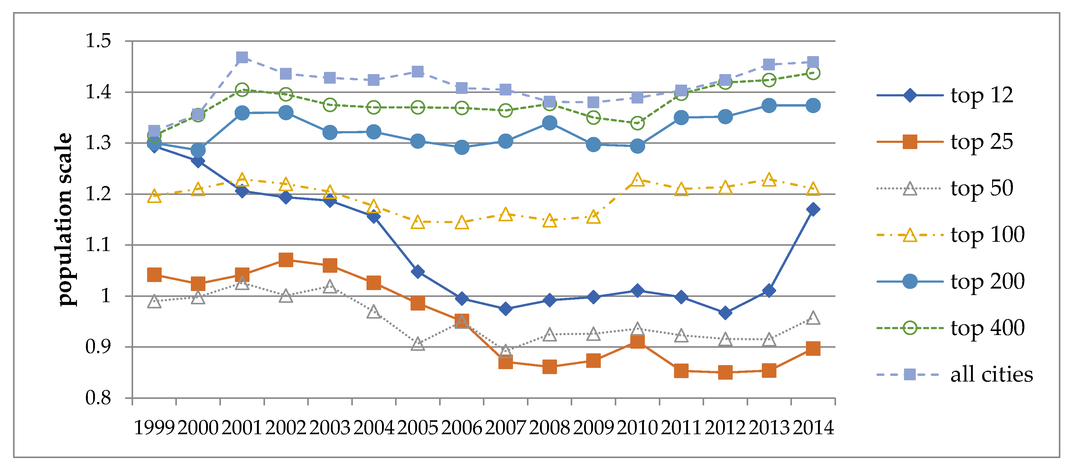
Figure 1 shows the trends of the scale exponents of violent crime counts for the same seven subgroups of cities from 1999 to 2014. The four subgroups of 100 cities to all cities display a moderate increase in scale exponents over time, whereas the two subgroups of 25 and 50 cities display a moderate decline in their scale exponents. The one exception is the subgroup of 12 cities, displaying a more abrupt up and down fluctuation during the period.
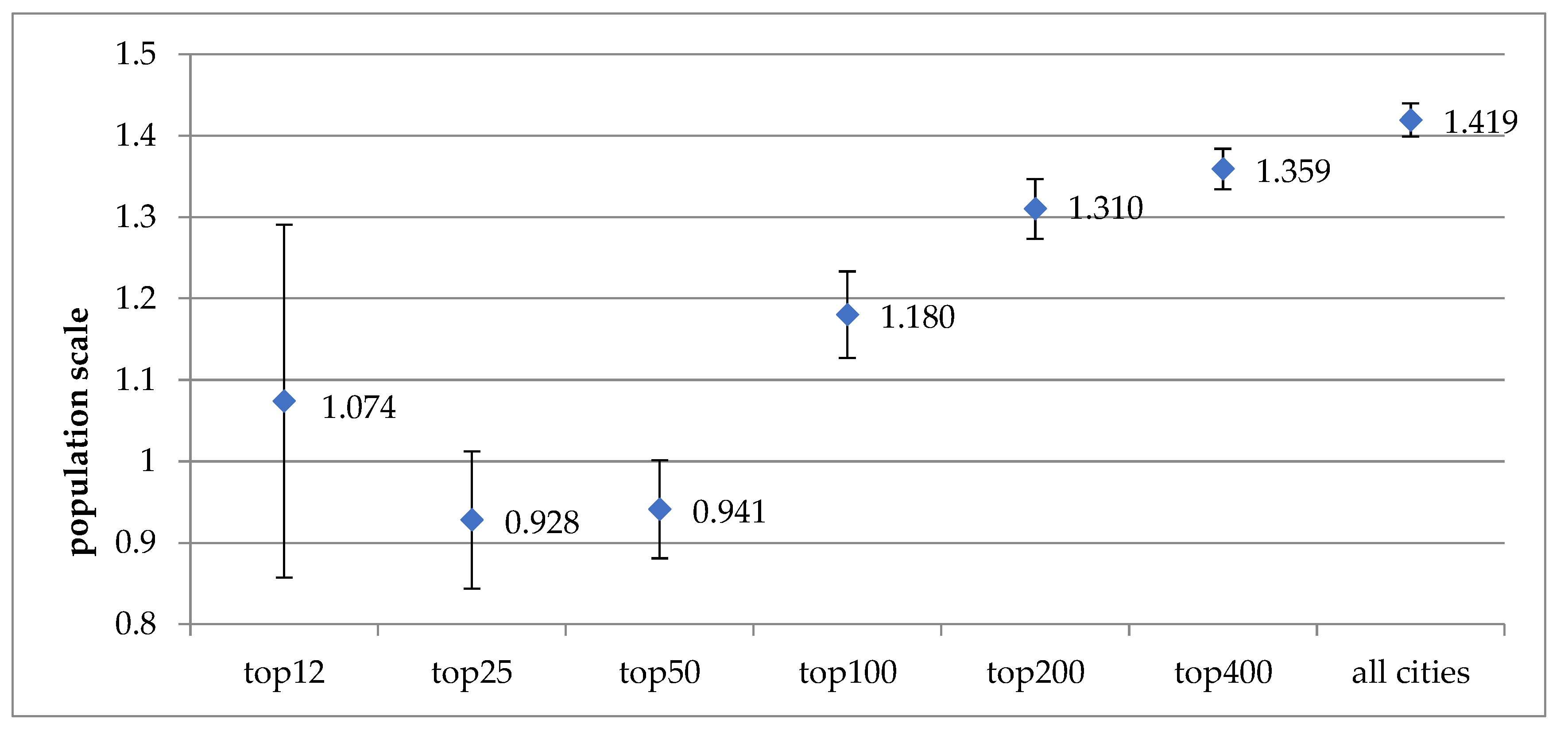
The result of the panel data analysis of bivariate regressions on violent crime counts, as shown in Table 1, also supports the trend of sublinear relationships associated with the top 12, 25 and 50 cities, evolving toward stronger superlinear relationships beginning from the top 100 cities toward all of the 755 cities. The lowest value of the exponents from the panel data analysis is 0.928 for the top 25 cities, which increases to 1.18 for the top 100 cities, 1.359 for the top 400 cities, and eventually increases to 1.459 for all 755 cities, as displayed in Figure 2.
The same type of yearly cross-sectional bivariate regressions of property crime counts for all cities show moderate superlinear relationships during 1999 to 2014, compared to the results from violent crime counts. The maximum value of the exponents is 1.229 in 2001, and the minimum value is 1.102 in 2000. The R2 for yearly regressions ranges from 0.651 to 0.794 with a median of 0.783. Table 2 shows that all 16 exponents are statistically significant at less than the 1% level. The number of cities analyzed ranges from the minimum of 504 cities in 1999, to the maximum of 755 cities in 2014.
The cross-sectional bivariate regressions for the top 12 cities, however, show sublinear relationships in a majority of the years analyzed, with only two years in which the scale exponents showed linear relationships—2000 and 2001. The maximum value of the exponents in 2001 is 1.011, while the minimum value of the exponents is 0.656 in 2013, indicating a strong sublinear relationship. All 16 exponents are statistically significant at less than the 5% or 1% level.
The results from the regressions for the top 25 cities generated even stronger sublinear relationships for each year, without exception. The maximum value of the exponents is 0.837 in 2002, while the minimum value is 0.671 in 2006, representing the strongest sublinear relationship. Once again, all 16 exponents are statistically significant at less than the 1% level. The results for the top 50 cities once again show sublinear relationships for every year. However, the sublinear relationships are more moderate compared to the results from the top 25 cities. The maximum value increases to 0.884 in 2002, while the minimum value also increases to 0.749 in 2000.
Moving to the results from the top 200 and top 400 cities, the values of the scale exponents return to superlinear relationships. For example, the maximum values of the exponents are 1.169 in 2000 and 1.213 in 2001, while the minimum values are 1.072 in 2009 and 1.123 in 2010 for the top 200 and top 400 cities, respectively. In other words, these maximum and minimum values begin to approach those superlinear exponents estimated for all 504 and 755 of the cities. All of the 112 exponents are statistically significant at less than the 5% level or 1% level.
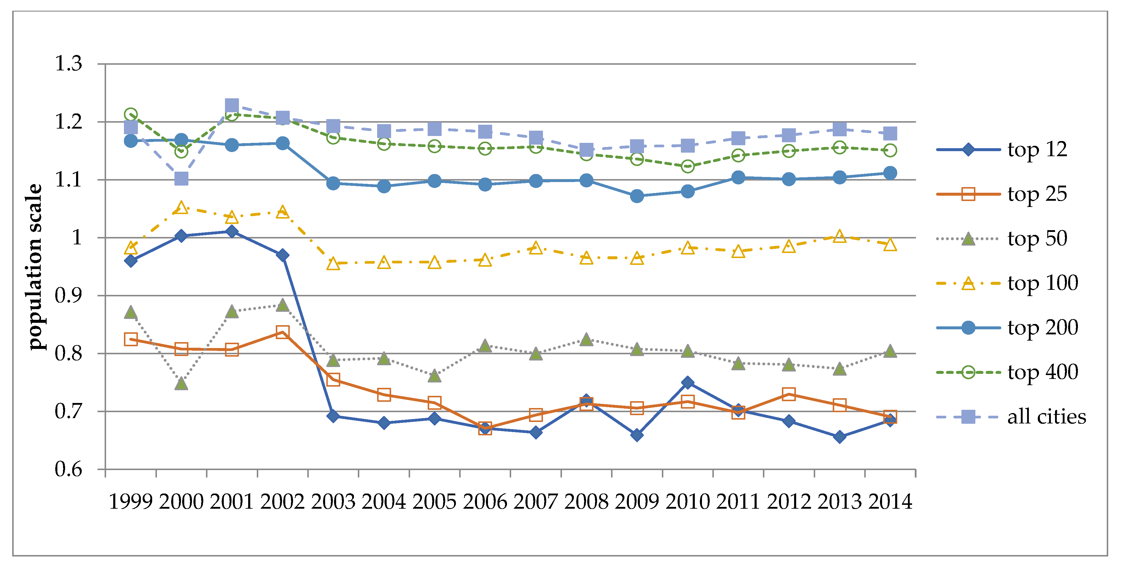
Figure 3 displays the trends of changing scale exponents for property crime for the same seven subgroups of cities during 1999 to 2014. Similar to violent crime, the top 25 and 50 cities display moderate declines in their exponents of property crime counts. However, the four subgroups of the top 100, top 200, top 400, and all cities display more or less stationary trends. Only the top 12 cities display an abrupt decline in the year 2003, followed by a more stationary trend thereafter.
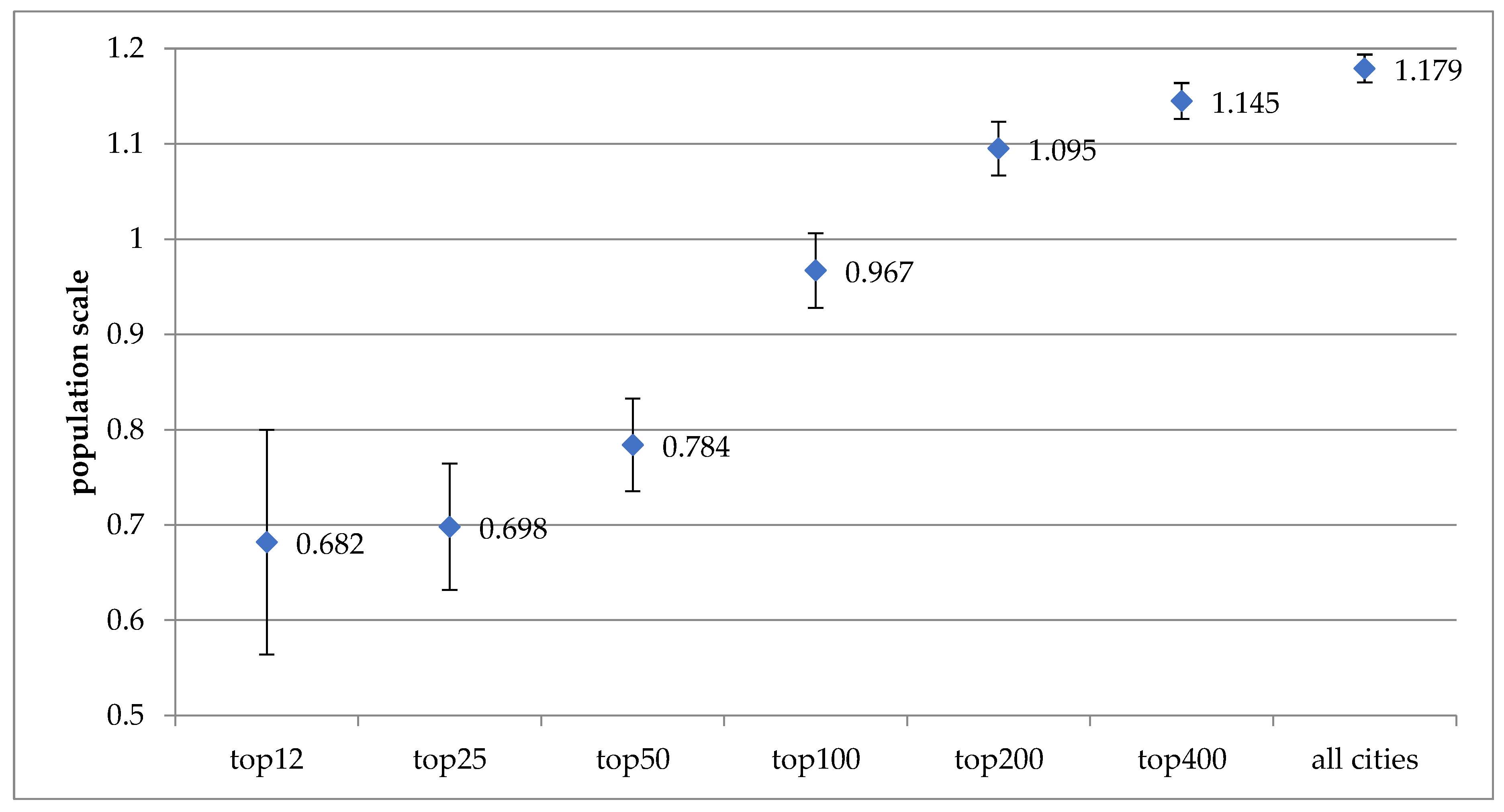
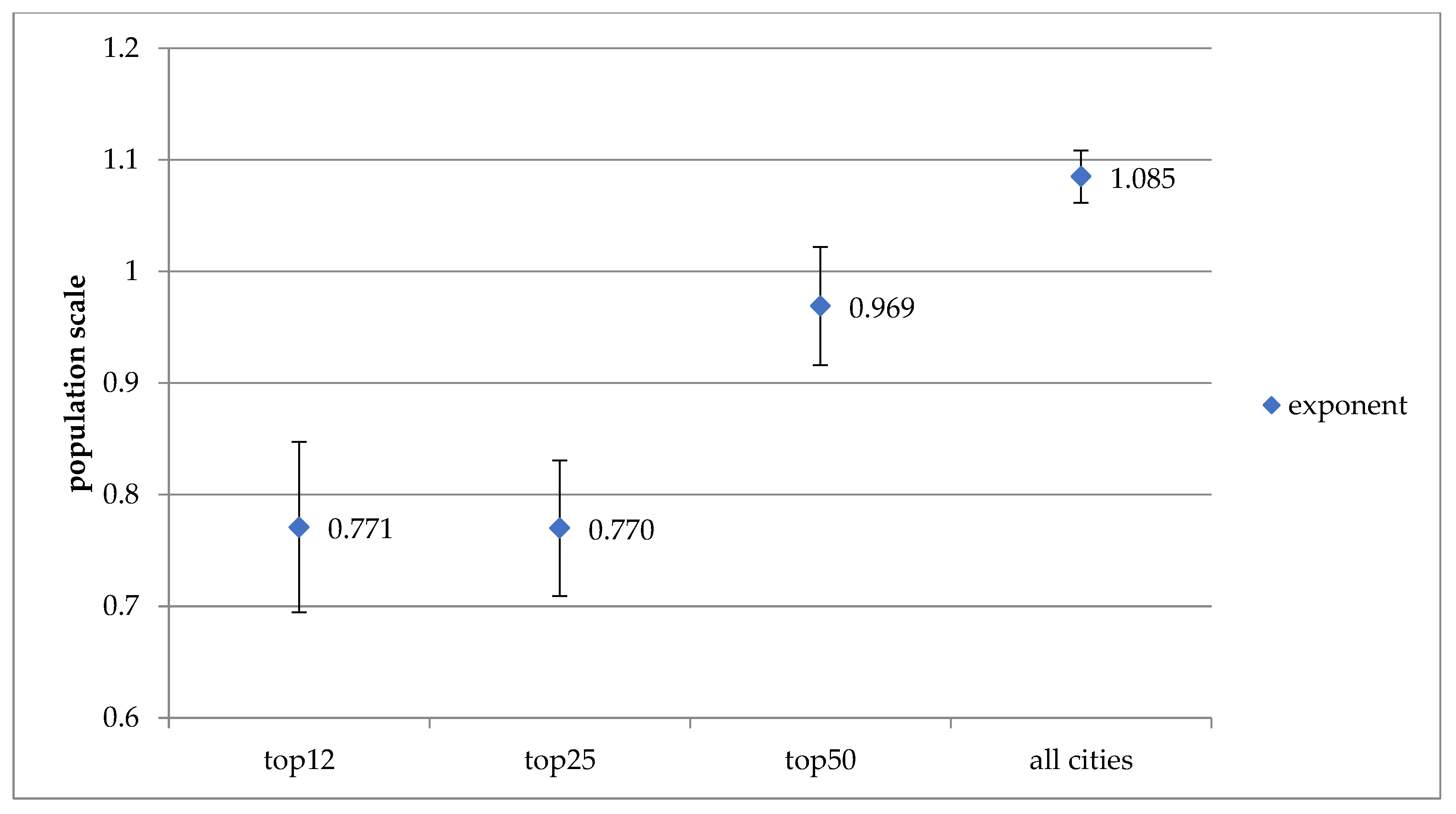
The result of panel data analysis on property crime counts, as shown in Table 2, also supports the trend of strong sublinear relationships associated with the top 12, 25, 50 and 100 cities, evolving towards moderate superlinear relationships beginning from the top 200 cities. More specifically, the exponent value of 0.682 associated with the top 12 cities increases to 0.784 for the top 50 cities, 0.967 for the top 100 cities, and then increases further to 1.095 for the top 200 cities, 1.145 for the top 400 cities, and finally to 1.179 for all cities, as displayed in Figure 4.
In summary, the results of bivariate regressions indicate that the values of the scale exponents decrease as the number of cities under analysis decreases. This finding applies to both violent and property crime counts. However, the type of scale relationship between crime counts and population size of cities varies by the type of crime. In the case of violent crime, the strong superlinear relationships associated with the subgroups of many cities evolve toward linear and moderate sublinear relationships for the subgroups of fewer cities, including the top 50 to top 12 cities. In the case of property crime, the moderate superlinear relationships associated with groups of many cities evolve toward strong sublinear relationships for the subgroups of fewer cities, including the top 100 to top 12 cities.
To provide a robustness check for these findings, the panel data analysis of multiple regressions for both violent and property crime counts are conducted. The additional control variables introduced are income per capita and population density. Due to missing data, however, the number of cities selected for multivariate analysis is much smaller compared to the number of cities analyzed in the bivariate regression.
The results from the panel data analysis of multiple regressions, shown in Table 3, for violent crime counts for the group of all cities, indicate that the scale exponent of the population size of the group of all cities is 1.22. The coefficients for income per capita and population density are −0.455 and +0.299. All three coefficients are statistically significant at less than the 1% level. These findings indicate that the violent crime count as a function of population size is superlinear when the impact from income and density is held constant. As for the impact from income, the well-to-do cities experience fewer violent crimes when impacts from the two other factors are held constant. In terms of the impact from density, high density cities experience higher violent crime counts when other factors are held constant. The results of the multiple regression from 1999 and ending in 2014 shows that the statistically significant scale exponents of the population are also superlinear, at 1.156 and 1.249, respectively. However, the coefficients for income and density are not statistically significant.
The results from the same type of analysis for the next group of 50 populous cities show that statistically significant scale coefficients of the population for the penal data is again superlinear, at 1.155. Coefficients associated with density are also statistically significant, but this is not the case for income. The yearly scale exponents for 2014 and 1999 are also statistically significant, at 1.163 and 1.196 respectively.
The results from the next group of the 25 most populous cities generate a statistically significant population scale exponent from the penal data at 0.818, representing a strong sublinear relationship. The coefficients associated with income and density are also statistically significant, with the same signs. The yearly scale exponents for 2014 and 1999 are again significant at 1.03 and 0.855, respectively.
Finally, the results from the 12 most populous cities produce a statistically significant population exponent at 0.875, which is again a clear-cut sublinear relationship from the panel data. The yearly population exponents are statistically significant at 0.830 and 1.194, respectively, for 2014 and 1999.
The coefficients associated with income and density are again statistically significant, with the same sets of signs. Figure 5 displays the trend of evolving population scale exponents from the panel data analysis of multiple regression, moving from clear-cut sublinear relationships for the 12 and 25 most populous cities, toward superlinear relationships for the 50 most populous cities, and for all cities under analysis.
The results from the panel data analysis of multiple regressions for property crime counts in Table 4 indicate that the population exponent is statistically significant, at 1.085 for all cities. The statistically significant coefficients of income and density are, respectively, −0.372 and −0.048. These results indicate that property crime counts as a function of population size are linear when the impact from income and density are held constant. As for the impact from income, rich cities experience lower property crime counts when the two other factors are held constant. Similarly, the more densely populated cities experience slightly lower property crime counts when the two other factors are held constant. The results from the multiple regressions for the years of 1999 and 2014 generate statistically significant population exponents, at 1.128 and 1.087 respectively.
The results from the next group of 50 most populous cities generate a statistically significant population exponent from the panel data at 0.969, representing a sublinear relationship. However, the coefficients associated with income and density are not statistically significant. The yearly statistically significant population exponents are 0.971 and 0.994 for the years of 2014 and 1999, respectively. The results from the next group of 25 most populous cities again produces a statistically significant population exponent at 0.77 from the panel data, representing a strong sublinear relationship. The coefficients associated with income and density are also statistically significant, with a negative coefficient for income. The yearly population exponents are 0.744 from 2014 and 0.875 from 1999, both of which are statistically significant.
Lastly, the results from the 12 most populous cities generate a statistically significant population exponent of 0.771, which represents another strong sublinear relationship. Statistically significant coefficients for income and density are also derived, with a negative sign for income. The yearly statistically significant populations exponents for property crime counts are 0.667 from 2014 and 0.818 from 1999. Figure 6 displays the trend of changing population exponents from the panel data analysis, moving from strong sublinear relationships associated with the 12 and 25 most populous cities toward a linear relationship for all cities in the sample group.
In short, the results from the multivariate analyses are similar to the earlier findings from bivariate analyses, which generated a changing trend of population scale exponents as the number of cities under analysis changed from the few most populous cities to many cities of varying population size. In the case of violent crime, the relationship changes from sublinear to superlinear. In the case of property crime, the relationship changes from strongly sublinear to linear. Thus, the results from multivariate analyses, as a robustness test, tend to support the results obtained earlier from the bivariate analyses.
5. Discussion
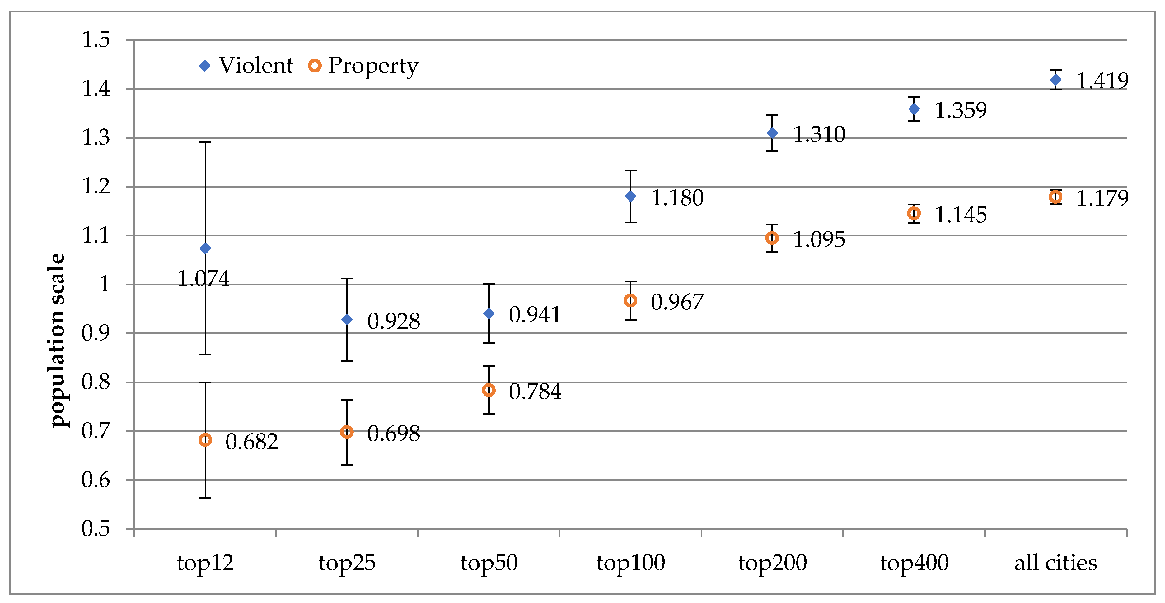
The key findings from our analysis can be summarized in Figure 7 and Figure 8. Figure 7 compares the population scale exponents of violent and property crime counts from the panel data analysis of the bivariate regressions, which are categorized according to the seven subgroups of cities with varying population sizes. On the other hand, Figure 8 compares the population scale exponents of violent and property crime counts from the panel data analysis of the multiple regressions, which are categorized according to the four subgroups which contain a much smaller number of cities.
Figure 7 summarizes several important findings from this study. First, the population exponents from the bivariate regression of the panel data display superlinear relationships for violent crime, as well as for property crime, for the total group of about 760 cities. Second, the superlinear relationship for violent crime counts at the exponent of 1.419 is much higher than the more moderate superlinear relationship for property crime counts at the exponent of 1.179. Both of these findings are in support of the findings from earlier studies [2,13]. Third, the values of the population exponents of violent and property crime counts from the subgroup of the top 400 and top 200 cities are quite similar to those estimated for the total group of all cities, showing strong superlinear relationships for violent crime, and moderate superlinear relationships for property crime. Fourth, the scale exponent for violent crime changes from a strong superlinear relationship to a superlinear relationship for the subgroup of the top 100 cities, while the superlinear relationship of property crime changes to a linear relationship.
Fifth, when the number of cities in the subgroup is further reduced to the top 50, top 25, and top 12 cities, the scaling relationship for violent crimes becomes moderately sublinear, while the relationship for property crime changes to strongly sublinear. Sixth, the values of the population exponents derived for violent crime exceed those derived for property crime counts, without exception. Nearly all the population exponents are statistically significant at less than the 5% or 1% level.
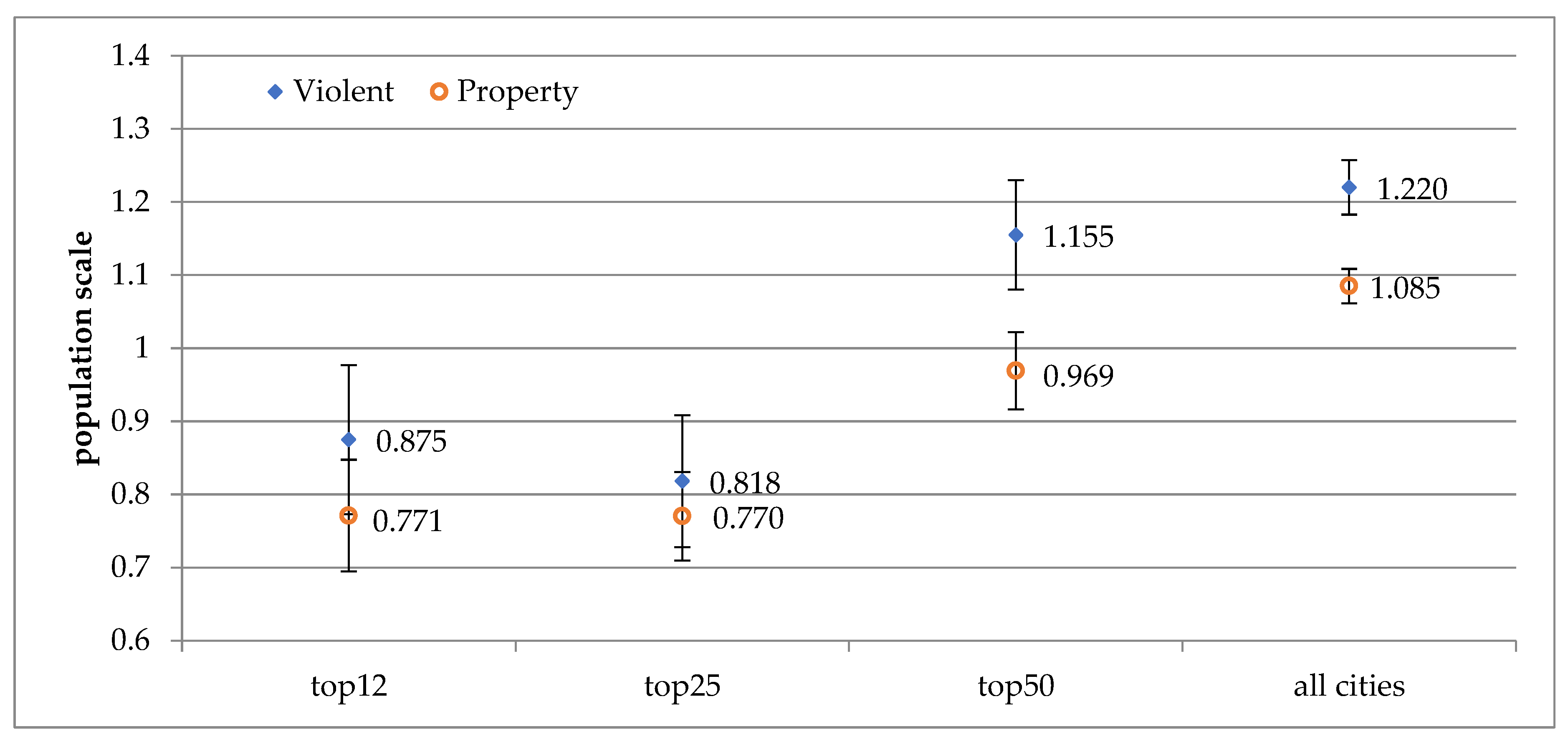
Figure 8 summarizes several findings in support of the findings shown in Figure 7. First, both population exponents from the multiple regression of the panel data generate superlinear relationships for violent and property crime for the much smaller total group of all cities, at about 120 cities. Second, the scale exponent of violent crime changes from a superlinear relationship to a sublinear relationship when the sample subgroup is reduced to 25 and 12 populous cities. For property crime, the scale relationship becomes strongly sublinear under the subgroups of 25 and 12 populous cities.
Third, the values of the population exponent derived for violent crime exceed those derived for property crime, without exception. Furthermore, the values of the population exponent from the multivariate analysis are somewhat smaller than those estimated from the bivariate analysis. Fourth, all the population exponents from the multivariate analysis are statistically significant. Furthermore, the coefficients associated with the two other control variables, income per capita and population density, are statistically significant with a few exceptions. The sign of the coefficient for income is always negative, while the sign of the coefficient for density is always positive.
Among these multiple findings, perhaps the most important is the fact that the variations of the population scale among subgroups are so much wider than expected. In the bivariate analysis, the maximum value of the population exponent is 1.419 for violent crime, derived from the total group of all cities, whereas the minimum is 0.928 from the subgroup of the top 25 cities. Thus, the maximum difference between the two exponents is 0.491, which means about a 40.5% difference in violent crime counts for every 100% difference in population size between these two subgroups of cities. In the multivariate analysis, the maximum difference is somewhat less at 0.402, which still means about a 32% difference of violent crime counts as a function of doubling the population size between the two subgroups of cities.
In terms of policy implications, the findings from this research establish the advantageous position for individual cities whose population sizes are large enough to position themselves within the top 50 cities. These cities can expect relatively fewer crime counts to occur, resulting from a future population increase. In the case of violent crime counts, a 100% increase in population size may generate about a 92% increase in crime counts derived from the population exponent of 0.941. In the case of property crime counts, a 100% increase in population may generate about a 72.2% increase (derived from a population exponent of 0.784) in property crime counts. Furthermore, they can implement a set of policy options to keep their cities attractive, so that their future population continues to grow. The results from our multivariate analysis suggest that maintaining the growth of income per capita, and reducing population density in their cities, can also help to lessen the number of crime counts.
If the population size of individual cities is smaller, placing them into the top 100 or top 200 cities, scaling relations from this research indicate that they would be in a somewhat disadvantageous position of a moderate superlinear relationship in the case of violent crime counts. In property crime counts, they would be in a neutral position with a linear relationship. In other words, a 100% increase in population is likely to increase their property crime counts.
In short, an individual city of any population size can use the scaling relationship developed in this study to project how many more crime counts can be expected in the future, based on their projected future population increase. Furthermore, the resource allocation system for law enforcement, criminal justice systems, and other crime prevention measures may incorporate the most appropriate scaling relationships associated with the particular population size of the city involved.
There are several limitations to this research, each of which can be suggested as a topic for future research. One such limitation deals with the lack of comprehensive treatment of multiple control variables in the multivariate analysis. For example, such control variables as the unemployment rate, percentage of males divorced, the Gini index, the percent of the population size aged 15–29, poverty, native-born status, residential stability, and many others have been used as additional variables in other research [54,55,56]. Another limitation deals with the fact that the coverage of this study is limited to cities in the U.S.
Despite these limitations, this research has provided in-depth empirical evidence in support of the proposition that the bigger the city, the lower its crime rates.
Author Contributions
The authors contributed to the development, implementation, analysis and writing of this study as follows: conceptualization, methodology, and analysis, Y.S.C.; writing—original draft preparation, Y.S.C. and H.E.K.; writing—review and editing, H.E.K. and S.M.J.
Funding
This research received no external funding.
Acknowledgments
We are grateful to Won Joung Kim, a research assistant at Gachon Center of Convergence Research for his contribution in preparing this manuscript.
Conflicts of Interest
The authors declare no conflict of interest.
References
- Braithwaite, J. Population growth and crime. Aust. N. Z. J. Criminol. 1975, 8, 57–60. [Google Scholar] [CrossRef]
- Glaeser, E.; Sacerdote, B. Why is there more crime in cities? J. Pol. Econ. 1999, 107, S225–S258. [Google Scholar] [CrossRef]
- James, N. Recent Violent Crime Trends in the United States; R45236; Congressional Research Service: Washington, DC, USA, 2008.
- Litman, T. Transportation and public health. Annu. Rev. Publ. Health 2013, 34, 217–233. [Google Scholar] [CrossRef] [PubMed]
- Kneebone, E.; Raphael, S. City and Suburban Crime Trends in Metropolitan America; Brookings: Washington, DC, USA, 2011. [Google Scholar]
- Bettencourt, L.M.A.; Lobo, J.; West, G.B. The self-similarity of human social organization and dynamics in cities. In Complexity Perspectives in Innovation and Social Change; Lane, D., Pumain, D., van der Leeuw, S.E., West, G., Eds.; Springer: Cham, Switzerland, 2009; Volume 7, pp. 221–236. [Google Scholar]
- Land, K.C.; McCall, P.L.; Cohen, L.E. Structural covariates of homicide rates: Are there any invariance across time and social space? Am. J. Sociol. 1990, 95, 923–963. [Google Scholar] [CrossRef]
- Ackerman, W.E. Socioeconomic correlates of increasing crime rates in smaller communities. Prof. Geogr. 1998, 50, 372–387. [Google Scholar] [CrossRef]
- Ousey, G. Explaining regional and urban variation in crime: A review of research. In Criminal Justice; The Nature of Crime: Continuity and Change; LaFree, G., Ed.; U.S. Department of Justice: Washington, DC, USA, 2000; Volume 1, pp. 261–308. [Google Scholar]
- Bettencourt, L.M.A.; Lobo, J.; Helbing, D.; Kuhnert, C.; West, G.B. Growth, innovation, scaling, and the pace of life in cities. Proc. Natl. Acad. Sci. USA 2007, 104, 7301–7306. [Google Scholar] [CrossRef] [PubMed] [Green Version]
- Bettencourt, L.M.A. The origins of scaling in cities. Science 2013, 340, 1438–1441. [Google Scholar] [CrossRef]
- Gomez-Lievano, A.; Youn, H.; Bettencourt, L.M.A. The statistics of urban scaling and their connection to Zipf’s law. PLoS ONE 2012, 7, e40393. [Google Scholar] [CrossRef]
- Choi, S.B.; Lee, Y.J.; Chang, Y.S. Population size and urban health advantage: Scaling analyses of four major diseases for 417 US counties. Int. J. Soc. Syst. Sci. 2018, 10, 35–55. [Google Scholar] [CrossRef]
- Wirth, L. Urbanism as a way of life. Am. J. Sociol. 1938, 44, 1–24. [Google Scholar] [CrossRef]
- Fischer, C.S. Toward a subcultural theory of urbanism. Am. J. Sociol. 1975, 80, 1319–1341. [Google Scholar] [CrossRef]
- Fischer, C.S. The subcultural theory of urbanism: A twentieth-year assessment. Am. J. Sociol. 1995, 101, 543–577. [Google Scholar] [CrossRef]
- Tittle, C.R. Influences on urbanism: A test of predictions from three perspectives. Soc. Probl. 1989, 36, 270–288. [Google Scholar] [CrossRef]
- Simmel, G. The Sociology of Georg Simmel; Wolff, K.H., Translator; The Free Press: Glencoe, UK, 1950. [Google Scholar]
- Mayhew, B.; Levinger, R. Size and the density of interaction in human aggregates. Am. J. Sociol. 1976, 82, 86–110. [Google Scholar] [CrossRef]
- Cohen, L.E.; Felson, M. Social change and crime rate trends: A routine activity approach. Am. Sociol. Rev. 1979, 44, 588–608. [Google Scholar] [CrossRef]
- Felson, M.; Clarke, R.V.G. Opportunity Makes the Thief: Practical Theory for Crime Prevention; Policing and Reducing Crime Unit, Home Office: London, UK, 1998; Available online: https://pdfs.semanticscholar.org/09db/dbce90b22357d58671c41a50c8c2f5dc1cf0.pdf (accessed on 15 February 2019).
- Newman, P.; Kenworthy, J.R. Gasoline consumption and cities. J. Am. Plan. Assoc. 1989, 55, 24–37. [Google Scholar] [CrossRef]
- Kenworthy, J.R.; Laube, F.B. Patterns of automobile dependence in cities: An international overview of key physical and economic dimensions with some implications for urban policy. Transport. Res. A-Pol. 1999, 33, 691–723. [Google Scholar] [CrossRef]
- Chang, Y.S.; Lee, Y.J.; Choi, S.B. Is there more traffic congestion in larger cities? –Scaling analysis of the 101 largest U.S. urban centers. Transport. Policy 2017, 59, 54–63. [Google Scholar] [CrossRef]
- Gordon, P.; Richardson, H.W.; Jun, M. The commuting paradox evidence from the top twenty. J. Am. Plan. Assoc. 1991, 57, 416–420. [Google Scholar] [CrossRef]
- Louf, R.; Barthelemy, M. Scaling: Lost in the smog. Environ. Plan. B 2014, 41, 767–769. [Google Scholar] [CrossRef]
- Vlahov, D.; Galea, S.; Freudenberg, N. Urban health-toward an urban health advantage. J. Public Health Man 2005, 11, 256–258. [Google Scholar]
- Kawachi, I.; Berkman, L.F. Social ties and mental health. J. Urban Health 2001, 78, 458–467. [Google Scholar] [CrossRef]
- Owen, N.; Humpel, N.; Leslie, E.; Bauman, A.; Sallis, J.F. Understanding environmental influences on walking: Review and research agenda. Am. J. Prev. Med. 2004, 27, 67–76. [Google Scholar] [CrossRef] [PubMed]
- Lee, R.E.; Cubbin, C. Neighborhood context and youth cardiovascular health behaviors. Am. J. Public Health 2002, 92, 428–436. [Google Scholar] [CrossRef] [PubMed]
- Brown, M.A.; Southworth, F.; Sarzynski, A. Shrinking the Carbon Footprint of Metropolitan America; Brookings Institution: Washington, DC, USA, 2008. [Google Scholar]
- Dodman, D. Blaming cities for climate change? An analysis of urban greenhouse gas emissions inventories. Environ. Urban 2009, 21, 185–201. [Google Scholar] [CrossRef] [Green Version]
- Hoornweg, D.; Sugar, L.; Lorena, C.; Gomez, C.L.T. Cities and greenhouse gas emissions: Moving forward. Environ. Urban 2011, 23, 207–227. [Google Scholar] [CrossRef]
- Kennedy, C.; Demoullin, S.; Mohareb, E. Cities reducing their greenhouse gas emissions. Energy Policy 2012, 49, 774–777. [Google Scholar] [CrossRef]
- Satterthwaite, D. Cities contribution to global warming: Notes on the allocation of greenhouse gas emissions. Environ. Urban 2008, 20, 539–549. [Google Scholar] [CrossRef]
- Muller, N.Z.; Jha, A. Does environmental policy affect scaling laws between population and pollution? Evidence from American metropolitan areas. PLoS ONE 2017, 12, e0181407. [Google Scholar] [CrossRef]
- Oliveira, E.A.; Andrade, J.S., Jr.; Makse, H.A. Large cities are less green. Sci. Rep. 2014, 4, 4235. [Google Scholar] [CrossRef] [Green Version]
- Marcotullio, P.J.; Sarzynski, A.; Albrecht, J.; Schulz, N.; Garcia, J. The geography of global urban greenhouse gas emissions: An exploratory analysis. Clim. Chang. 2013, 121, 621–634. [Google Scholar] [CrossRef]
- Rybski, D.; Reusser, D.E.; Winz, A.L.; Fichtner, C.; Sterzel, T.; Kropp, J.P. Cities as nuclei of sustainability? Environ. Plan. B 2015, 44, 425–440. [Google Scholar] [CrossRef]
- Nolan, J. Establishing the statistical relationship between population size and UCR crime rate: Its impact and implications. J. Crim. Justice 2004, 32, 547–555. [Google Scholar] [CrossRef]
- Planetizen. Available online: https://www.planetizen.com/node/65857 (accessed on 21 March 2019).
- Bettencourt, L.M.A.; Lobo, J.; Strumsky, D.; West, G.B. Urban scaling and its deviations: Revealing the structure of wealth, innovation and crime across cities. PLoS ONE 2010, 5, e13541. [Google Scholar] [CrossRef]
- Beck, N.; Katz, J.N. What to do (and not to do) with time-series cross-section data. Am. Pol. Sci. Rev. 1995, 89, 634–647. [Google Scholar] [CrossRef]
- Dietz, T.; Rosa, E.A. Rethinking the environmental impacts of population, affluence and technology. Hum. Ecol. Rev. 1994, 1, 277–300. [Google Scholar]
- York, R.; Rosa, E.A.; Dietz, T. STIRPAT, IPAT and ImPACT: Analytic tools for unpacking the driving forces of environmental impacts. Ecol. Econ. 2003, 46, 351–365. [Google Scholar] [CrossRef]
- Ehrlich, P.; Holdren, J. A bulletin dialogue on the ‘closing circle’: Critique: One- dimensional ecology. B Atom. Sci 1972, 28, 16–27. [Google Scholar] [CrossRef]
- York, R.; Rosa, E.A.; Dietz, T. Footprints on the earth: The environmental consequences of modernity. Am. Sociol. Rev. 2003, 68, 279–300. [Google Scholar] [CrossRef]
- FBI. Available online: https://ucr.fbi.gov/crime-in-the-u.s/ (accessed on 4 July 2018).
- BEA. Personal Income by County, Metro, and Other Areas. Available online: https://www.bea.gov/data/income-saving/personal-income-county-metro-and-other-areas (accessed on 10 November 2018).
- Kvalseth, T. A note on the effects of population density and unemployment on urban crime. Criminology 1977, 15, 105–110. [Google Scholar] [CrossRef]
- Shichor, D.; Decker, D.; O’Brien, R. Population density and criminal victimization. Criminology 1979, 17, 184–193. [Google Scholar] [CrossRef]
- Christens, B. Predicting violent crime using urban and suburban densities. Behav. Soc. Issues 2005, 14, 113–127. [Google Scholar] [CrossRef]
- Harries, K. Property Crimes and Violence in United States: An Analysis of the influence of Population density. Int. J. Crim. Justice Sci. 2006, 1, 24–34. [Google Scholar]
- Rotolo, T.; Tittle, C. Population size, change, and crime in U.S. cities. J. Quant. Criminol. 2006, 22, 341–367. [Google Scholar] [CrossRef]
- Dennett, A.; Stillwell, J. Internal migration in Britain, 2000-01, examined through an area classification framework. Popul. Space Place 2010, 19, 517–538. [Google Scholar] [CrossRef]
- Boiving, R.; Felson, M. Crimes by visitors versus crimes by residents: The influence of visitor inflows. J. Quant. Criminol. 2018, 34, 465–480. [Google Scholar] [CrossRef]
Figure 1.
Scale exponents for violent crime counts from annual bivariate analyses for seven subgroups of cities (1999~2014).
Figure 1.
Scale exponents for violent crime counts from annual bivariate analyses for seven subgroups of cities (1999~2014).

Figure 2.
Scale exponents for violent crime counts from bivariate panel data analyses for seven subgroups of cities (1999~2014).
Figure 2.
Scale exponents for violent crime counts from bivariate panel data analyses for seven subgroups of cities (1999~2014).

Figure 3.
Scale exponents for property crime counts from annual bivariate analyses for seven subgroups of cities (1999~2014).
Figure 3.
Scale exponents for property crime counts from annual bivariate analyses for seven subgroups of cities (1999~2014).

Figure 4.
Scale exponents for property crime counts from bivariate panel data analyses for seven subgroups of cities (1999~2014).
Figure 4.
Scale exponents for property crime counts from bivariate panel data analyses for seven subgroups of cities (1999~2014).

Figure 5.
Scale exponents for violent crime counts from multivariate panel data analyses for the smaller four subgroups of cities (1999~2014).
Figure 5.
Scale exponents for violent crime counts from multivariate panel data analyses for the smaller four subgroups of cities (1999~2014).

Figure 6.
Scale exponents for property crime counts from the multivariate panel data analyses for the smaller four subgroups of cities (1999~2014).
Figure 6.
Scale exponents for property crime counts from the multivariate panel data analyses for the smaller four subgroups of cities (1999~2014).

Figure 7.
Scale exponents for violent and property crime counts from bivariate panel data analyses for seven subgroups of cities (1999~2014).
Figure 7.
Scale exponents for violent and property crime counts from bivariate panel data analyses for seven subgroups of cities (1999~2014).

Figure 8.
Scale exponents for violent and property crime counts from multivariate panel data analyses for the smaller four subgroups of cities (1999~2014).
Figure 8.
Scale exponents for violent and property crime counts from multivariate panel data analyses for the smaller four subgroups of cities (1999~2014).


Table 1.
Cross-sectional bivariate analyses of violent crime counts by seven subgroups of cities.
| Year | Scale Exponent | ||||||
|---|---|---|---|---|---|---|---|
| Top 12 Cities | Top 25 Cities | Top 50 Cities | Top 100 Cities | Top 200 Cities | Top 400 Cities | All Cities | |
| 1999 | 1.294 *** | 1.042 *** | 0.990 *** | 1.197 *** | 1.300 *** | 1.315 *** | 1.324 *** |
| 2000 | 1.265 *** | 1.024 *** | 0.998 *** | 1.210 *** | 1.286 *** | 1.355 *** | 1.356 *** |
| 2001 | 1.203 *** | 1.042 *** | 1.026 *** | 1.229 | 1.359 *** | 1.405 *** | 1.468 *** |
| 2002 | 1.194 ** | 1.071 *** | 1.001 *** | 1.220 | 1.360 *** | 1.396 *** | 1.436 *** |
| 2003 | 1.187 ** | 1.060 *** | 1.019 *** | 1.205 *** | 1.321 *** | 1.375 *** | 1.428 *** |
| 2004 | 1.156 ** | 1.026 *** | 0.970 *** | 1.177 *** | 1.322 *** | 1.370 *** | 1.424 *** |
| 2005 | 1.048 ** | 0.986 *** | 0.907 *** | 1.146 *** | 1.304 *** | 1.370 *** | 1.440 *** |
| 2006 | 0.995 ** | 0.951 *** | 0.950 *** | 1.145 *** | 1.292 *** | 1.369 *** | 1.408 *** |
| 2007 | 0.975 ** | 0.871 *** | 0.892 *** | 1.161 *** | 1.304 *** | 1.364 *** | 1.405 *** |
| 2008 | 0.992 ** | 0.861 *** | 0.925 *** | 1.149 *** | 1.340 *** | 1.377 *** | 1.381 *** |
| 2009 | 0.998 ** | 0.873 *** | 0.926 *** | 1.156 *** | 1.297 *** | 1.350 *** | 1.380 *** |
| 2010 | 1.011 ** | 0.911 *** | 0.936 *** | 1.229 *** | 1.294 *** | 1.339 *** | 1.389 *** |
| 2011 | 0.998 *** | 0.853 *** | 0.923 *** | 1.210 *** | 1.350 *** | 1.397 *** | 1.403 *** |
| 2012 | 0.967 *** | 0.850 *** | 0.916 *** | 1.214 *** | 1.352 *** | 1.419 *** | 1.424 *** |
| 2013 | 1.011 *** | 0.854 *** | 0.915 *** | 1.229 *** | 1.374 *** | 1.424 *** | 1.454 *** |
| 2014 | 1.170 *** | 0.897 *** | 0.958 *** | 1.211 *** | 1.374 *** | 1.438 *** | 1.459 *** |
| Panel Data | 1.074 *** | 0.928 *** | 0.941 *** | 1.180 *** | 1.310 *** | 1.359 *** | 1.419 *** |
** significant at the 5% level, *** significant at the 1% level.
Table 2.
Cross-sectional bivariate analyses of property crime counts for seven subgroups of cities.
| Year | Scale Exponent | ||||||
|---|---|---|---|---|---|---|---|
| Top 12 Cities | Top 25 Cities | Top 50 Cities | Top 100 Cities | Top 200 Cities | Top 400 Cities | All Cities | |
| 1999 | 0.960 ** | 0.825 *** | 0.872 *** | 0.983 *** | 1.167 *** | 1.213 *** | 1.191 *** |
| 2000 | 1.003 ** | 0.808 *** | 0.749 *** | 1.053 *** | 1.169 *** | 1.149 *** | 1.102 *** |
| 2001 | 1.011 ** | 0.807 *** | 0.873 *** | 1.036 *** | 1.160 *** | 1.213 *** | 1.229 *** |
| 2002 | 0.970 ** | 0.837 *** | 0.884 *** | 1.045 *** | 1.163 *** | 1.206 *** | 1.207 *** |
| 2003 | 0.692 ** | 0.755 *** | 0.789 *** | 0.956 *** | 1.094 *** | 1.173 *** | 1.193 *** |
| 2004 | 0.680 ** | 0.729 *** | 0.792 *** | 0.958 *** | 1.089 *** | 1.162 *** | 1.184 *** |
| 2005 | 0.688 ** | 0.715 *** | 0.762 *** | 0.958 *** | 1.098 *** | 1.158 *** | 1.188 *** |
| 2006 | 0.671 ** | 0.671 *** | 0.814 *** | 0.962 *** | 1.092 *** | 1.154 *** | 1.183 *** |
| 2007 | 0.664 ** | 0.694 *** | 0.800 *** | 0.983 *** | 1.098 *** | 1.157 *** | 1.173 *** |
| 2008 | 0.719 ** | 0.713 *** | 0.825 *** | 0.966 *** | 1.099 *** | 1.144 *** | 1.152 *** |
| 2009 | 0.659 ** | 0.706 *** | 0.808 *** | 0.965 *** | 1.072 *** | 1.136 *** | 1.158 *** |
| 2010 | 0.750 ** | 0.717 *** | 0.805 *** | 0.983 *** | 1.080 *** | 1.123 *** | 1.159 *** |
| 2011 | 0.702 ** | 0.698 *** | 0.783 *** | 0.977 *** | 1.104 *** | 1.142 *** | 1.172 *** |
| 2012 | 0.683 *** | 0.730 *** | 0.781 *** | 0.986 *** | 1.101 *** | 1.150 *** | 1.177 *** |
| 2013 | 0.656 *** | 0.711 *** | 0.774 *** | 1.003 *** | 1.104 *** | 1.156 *** | 1.187 *** |
| 2014 | 0.685 *** | 0.691 *** | 0.805 *** | 0.989 *** | 1.112 *** | 1.151 *** | 1.180 *** |
| Panel Data | 0.682 *** | 0.698 *** | 0.784 *** | 0.967 *** | 1.095 *** | 1.145 *** | 1.179 *** |
** significant at the 5% level, *** significant at the 1% level.
Table 3.
Cross-sectional panel data multivariate analysis of violent crime counts for the reduced four subgroups (1999–2014).
Table 3.
Cross-sectional panel data multivariate analysis of violent crime counts for the reduced four subgroups (1999–2014).
| Top 12 | Top 25 | Top 50 | All cities | |||||||||
|---|---|---|---|---|---|---|---|---|---|---|---|---|
| 1999 | 2014 | Panel Data | 1999 | 2014 | Panel Data | 1999 | 2014 | Panel Data | 1999 | 2014 | Panel Data | |
| Population | 1.194 *** (0.057) | 0.830 ** (0.170) | 0.875 *** (0.052) | 0.130 *** (0.097) | 0.855 *** (0.167) | 0.818 *** (0.046) | 1.196 *** (0.081) | 1.163 *** (0.132) | 1.155 *** (0.382) | 1.156 *** (0.056) | 1.249 *** (0.065) | 1.220 *** (0.019) |
| Income Per Capita | −1.102 *** (0.105) | −0.688 * (0.212) | −0.611 *** (0.063) | −0.593 ** (0.187) | −0.177 (0.262) | −0.396 *** (0.062) | −0.062 (0.280) | 0.061 (0.321) | −0.088 (0.067) | −0.071 (0.250) | −0.423 (0.247) | −0.445 *** (0.050) |
| Population Density | 0.449 ** (0.721) | 0.611 ** (0.151) | 0.581 *** (0.040) | −0.448 ** (0.128) | 0.526 ** (0.230) | 0.555 *** (0.041) | 0.203 (0.127) | 0.188 (0.195) | 0.034 *** (0.041) | 0.166 (0.095) | 0.165 (0.092) | 0.229 *** (0.257) |
| Constant | −0.794 (0.756) | −0.522 (1.132) | −1.644 * (0.726) | −2.766 (1.479) | −5.689 (2.833) | −0.963 *** (0.734) | −8.439 ** (2.559) | −9.577 ** (3.297) | −8.657 *** (0.758) | −7.529 ** (2.402) | −5.300 * (2.487) | −5.118 *** (0.525) |
| R2 | 0.982 | 0.879 | 0.965 | 0.915 | 0.743 | 0.907 | 0.831 | 0.755 | 0.787 | 0.813 | 0.770 | 0.714 |
* Significant at the 10% level, ** significant at the 5% level, *** significant at the 1% level. Standard errors of coefficient estimates appear in parentheses.
Table 4.
Cross-sectional panel data multivariate analysis of property crime counts for the reduced four subgroups (1999–2014).
Table 4.
Cross-sectional panel data multivariate analysis of property crime counts for the reduced four subgroups (1999–2014).
| Top 12 | Top 25 | Top 50 | All cities | |||||||||
|---|---|---|---|---|---|---|---|---|---|---|---|---|
| 1999 | 2014 | Panel Data | 1999 | 2014 | Panel Data | 1999 | 2014 | Panel Data | 1999 | 2014 | Panel Data | |
| Population | 0.818 *** (0.111) | 0.667 ** (0.140) | 0.771 *** (0.039) | 0.875 *** (0.104) | 0.744 *** (0.120) | 0.770 *** (0.031) | 0.994 *** (0.073) | 0.971 *** (0.081) | 0.969 *** (0.027) | 1.128 *** (0.044) | 1.087 *** (0.043) | 1.085 *** (0.012) |
| Income Per Capita | −0.527 (0.246) | −0.418 (0.221) | −0.510 *** (0.556) | −0.195 (0.131) | −0.116 (0.175) | −0.243 *** (0.047) | 0.016 (0.204) | −0.002 (0.201) | −0.073 (0.044) | −0.257 (0.140) | −0.162 (0.147) | −0.372 *** (0.029) |
| Population Density | 0.002 (0.098) | 0.311 (0.181) | 0.127 *** (0.029) | 0.057 (0.077) | 0.222 (0.135) | 0.088 ** (0.026) | −0.012 (0.084) | 0.003 (0.118) | −0.018 (0.026) | 0.050 (0.053) | −0.073 (0.060) | −0.048 ** (0.016) |
| Constant | −4.930 (3.001) | 3.053 * (1.264) | 4.321 *** (0.589) | 0.298 (0.173) | −0.548 (2.017) | 1.832 *** (0.485) | −2.887 (2.030) | −3.008 (2.362) | −1.808 *** (0.495) | −1.543 (1.605) | −2.157 (1.742) | 0.053 (0.331) |
| R2 | 0.882 | 0.810 | 0.979 | 0.866 | 0.818 | 0.958 | 0.849 | 0.838 | 0.914 | 0.871 | 0.881 | 0.855 |
* Significant at the 10% level, ** significant at the 5% level, *** significant at the 1% level. Standard errors of coefficient estimates appear in parentheses.
© 2019 by the authors. Licensee MDPI, Basel, Switzerland. This article is an open access article distributed under the terms and conditions of the Creative Commons Attribution (CC BY) license (http://creativecommons.org/licenses/by/4.0/).
Share and Cite
MDPI and ACS Style
Chang, Y.S.; Kim, H.E.; Jeon, S. Do Larger Cities Experience Lower Crime Rates? A Scaling Analysis of 758 Cities in the U.S. Sustainability 2019, 11, 3111. https://0-doi-org.brum.beds.ac.uk/10.3390/su11113111
AMA Style
Chang YS, Kim HE, Jeon S. Do Larger Cities Experience Lower Crime Rates? A Scaling Analysis of 758 Cities in the U.S. Sustainability. 2019; 11(11):3111. https://0-doi-org.brum.beds.ac.uk/10.3390/su11113111
Chicago/Turabian StyleChang, Yu Sang, Hann Earl Kim, and Seongmin Jeon. 2019. "Do Larger Cities Experience Lower Crime Rates? A Scaling Analysis of 758 Cities in the U.S." Sustainability 11, no. 11: 3111. https://0-doi-org.brum.beds.ac.uk/10.3390/su11113111
Note that from the first issue of 2016, this journal uses article numbers instead of page numbers. See further details here.