1. Introduction
In the last few years, numerous researchers have studied the effects that the ongoing global crisis, triggered out by the US subprime in 2007, have determined not only on the economy, but also on the households’ daily habits. These phenomena have further confirmed the predominant role of the real estate sector in the economic activities of all the countries whose housing market is undoubtedly the main segment, and the peremptoriness to forecast future bubbles by appropriately measuring the changes of the economic and population fundamentals [
1,
2]. Not by chance, the rate of growth of housing prices has been included in the list of the indicators for the monitoring of the US economic imbalance [
3]. Furthermore, as highlighted by the analysis of Learne [
4], in the US eight of the previous ten recessions were started from substantial problems in the housing markets. In this context, some authors [
5] have pointed out that neglecting house price booms can have substantial impacts on the economy; other researchers have shown that important changes in housing prices could lead to significant modifications in household wealth [
6,
7,
8,
9,
10] and consequently drastic effects on psychological well-being of the community [
11].
The interrelation and the co-determination between the housing market and the macro-economy have been documented in several countries [
12,
13]. What is evident by comparing these studies is the extreme volatility of the housing market [
14,
15], and this contingence is responsible of the difficulty to obtain a spatial generalization of the main fundamentals that are able to explain housing market bubbles [
16,
17,
18,
19]. Therefore, a dynamic analysis of the macro-economic variables that can help to foresee sudden changes of the property values, in order to anticipate future real estate bubbles, should be developed in each specific territorial context.
2. Aim
This paper is presented in the framework outlined.
The research analyzes the functional relationships between the housing selling prices and the main socio-economic variables relating to five Spanish metropolitan areas (Barcelona, Bilbao, Madrid, Santiago de Compostela and Valencia), by implementing a methodology on the historical data sufficiently representative of the evolutions of the factors identified. The choice to analyze the Spanish context has been determined, first of all, by the constant predominant role of the housing market in this country’s economy, that is among the countries with the highest home ownership rate (around 80%); then, by the quick economic changes that have been affecting the Spanish country in the last decade, that after a period of containment of public spending and significant structural reforms in order to avoid the default risk caused by the crisis of the real estate sector and a youth unemployment rate that had reached 60%—has been appearing as one of the most dynamic European countries, with a GDP growth in 2017 around 3.7%, against 2.1% in Germany, 1.6% in France, 1.5% in Italy and 1.2% in the United Kingdom (
www.oecd.org).
The method proposed is a machine learning technique, able to exploit the actual functional relationships among the variables considered. The outputs obtained are models of simple interpretation, characterized by high statistical performance and compliance with the expected empirical phenomena, and that constitute a useful support for the forecast of the future housing market trends, generated by different evolutions of the socio-economic parameters identified by the models. For this reason, an empirical procedure for the construction of the future property value trends has been developed: the results highlight the forecasting and monitoring potentialities of the methodology, to be implemented (i) for public entities, interested in anticipating and checking future housing bubbles through appropriate economic policies, and (ii) for private operators interested in investing in the territory, in the phases of selection of the most attractive urban zones for new property realizations, (iii) for real estate investment trusts (REITs) and owners of large real estate portfolios, who could prepare the most effective strategies to sell or to enhance the property assets in view of future bubbles and bursts; (iv) for the credit institutions, which may organize more appropriate financing policies for investors and construction companies, taking into account the expected evolution of the property market.
The paper is divided into the following sections. In the third section the reference background on research that analyzes the correlations between the property market and the socio-economic factors is outlined. In the fourth section the case studies are presented: the demographic and territorial parameters are contextualized; the variables considered are specified and the main descriptive statistics are illustrated. In the fifth section the implemented methodology is explained, and the advantages of the algorithm used compared to classical machine learning techniques and multivariate dynamic regressions are highlighted. The sixth section reports the best models identified for the five case studies, in terms of statistical reliability and simplicity of the functional form, and the relationships of each model are interpreted. In the seventh section, a practical use of the models obtained is illustrated, which makes it possible to empirically predict the future market trends for each metropolitan area analyzed. Finally, in the eighth section the conclusions are discussed.
3. Background
The study of the interaction between the changes of socio-economic factors and the impacts on the housing prices has been the target of numerous investigations. These variables differ depending on the specific territorial context [
20,
21], but a comparison among the analysis carried out in the reference literature could highlight the main characteristics that affect the real estate trend over time.
Many authors have outlined the strong correlation between property prices and household income. Roback [
22] has pointed out that differences in housing prices across cities mainly depend on wage as well as urban amenity differences. Taltavull de la Paz [
23] has shown the relationship between residential prices and families’ waged income, as well as population growth and the productive structure, in Spanish cities. Fontenla et al. [
24] have concluded that both permanent and temporary income positively affect housing prices. Gibler et al. [
25] have outlined the predominance of the income among the variables characterized by a positive influence on the decision to move to a new house. At a macroeconomic level, the research of Filotto et al. [
26] has shown the correlation between the gross domestic product (GDP) and housing prices. Hoxha and Temeljotov Salaj [
27] have identified the most influencing factors on housing prices in Kosovo and Slovenia as GDP growth, real interest rates and construction costs. Wu et al. [
28] have stated that the expected export growth could significantly influence the growth rate of housing price.
Several authors have demonstrated the influence of population growth and unemployment rate on the changes of housing prices [
29]. The research carried out by Nistor and Reianu [
30] in Ontario cities (Canada) has highlighted that immigration and unemployment rate, as well as interest rate and income, are the main variables that explain housing prices. Sivitanides [
31] has illustrated the existence of a strong long-term relationship between housing prices and population growth, stating that any potential reduction of immigration and economic growth due to Brexit can limit house price increases. Muellbauer and Murphy [
32] have studied the impact of the housing stock and the population on the residential prices. Morano et al. [
33] have analyzed the contribution of the age of the population in Southern Italy on the changes of the property prices.
Land price is another variable identified as an important factor that influences housing prices [
34,
35]. Dreger and Zhang [
36] have reported the existence of a co-integration between actual housing price and actual land price, as well as actual per capital income and actual interest rate. Dachis et al. [
37] have analyzed the effect in Toronto (Canada) of the land transfer tax on housing prices. Montalvo and Vilchez [
38] have studied the effect of land use regulation on housing prices at municipal level.
The relationship between housing prices and rent has been also appropriately studied [
39,
40,
41]. Candas et al. [
42] have highlighted the significant impact of rent prices, as well as the land values, on housing prices. Montalvo [
43] has analyzed the determinants of housing price growth at the Spanish municipal level, concluding that rent prices have a statistically significant effect on residential prices.
The inverse correlation between mortgage rates and housing prices has been a research issue of several studies [
44,
45,
46]. Bover [
47] has demonstrated the main role of the credit sector on the housing market trends in Spain. Chen and Patel [
48] have outlined a long-term relationship in Taiwan between housing prices and interest rates. Liu et al. [
49] have shown the interaction between mortgage rates and housing prices in eight Australian cities. Habtewold Demewez [
50] has highlighted that mortgage rates are the main cause of changes in housing prices. Panagiotidis and Printzis [
51] have pointed out the fundamental weight of the mortgage-lending sector on the variations in housing prices in Greece and in South-east Europe.
Numerous authors have studied the sociological factors that affect the housing prices, such as age, gender, race and marital status [
52,
53,
54,
55]. Brasington [
56] has analyzed the relationship between housing prices and the proportion of white persons and serious crimes. Bowes and Ihlanfeldt [
57] have examined the influence on the housing prices of the percent of black residents and the density of crimes. Levy and Lee [
58] have studied the weight of the children on the housing purchase decision. Sabal [
59] has outlined the contribution of cultural factors on the housing prices in Spain, as well as of the population growth, the land prices and the investors’ expectations. Stoykova and Chou [
60] have assessed the impact of culture on housing prices, concluding that this aspect should be considered as a long-term housing price determinant. Lin et al. [
61] have detected the influence of the percentage of the elderly in the population, violent crime rates and foreclosure rates on the housing prices in the USA. Aswin Rahadiet al. [
62] emphasizes the importance of psychological factors, such as the closeness to the family, on the housing prices in Indonesia. Ge [
63] has studied the effects of ethnic changes on house prices. Tsatsaronis and Zhu [
64] have demonstrated that taxes and hereditary expectations are short-term housing price determinants in many countries. López García and Tajani et al. [
65,
66] have pointed out the influence of tax policies on the changes of housing prices respectively in Spain and in Italy.
4. Case Study
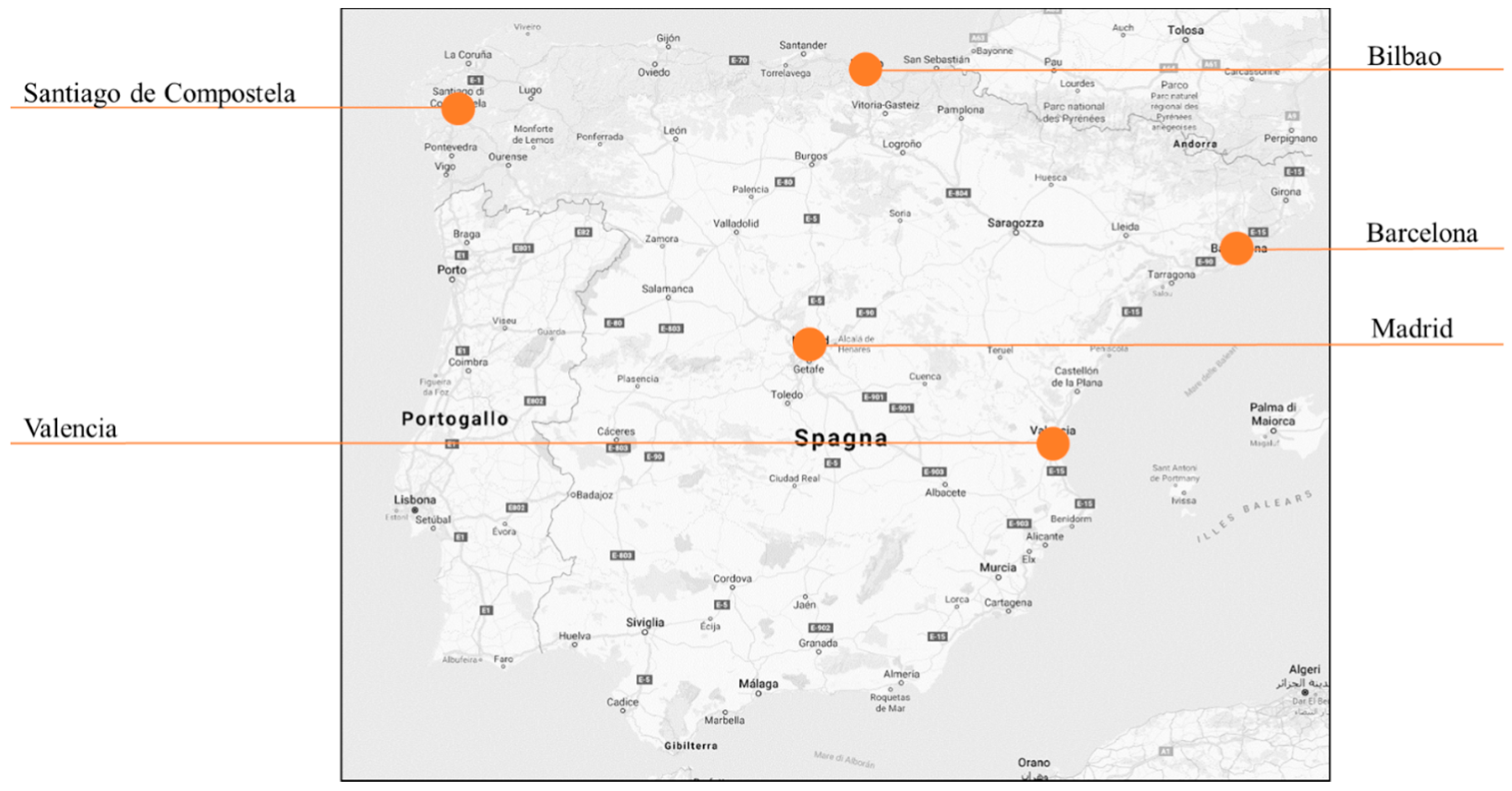
The case studies of this research concern the metropolitan areas of five Spanish cities: Barcelona, Bilbao, Madrid, Santiago de Compostela and Valencia. The analyzed cities are located in different geographical areas of Spain and are characterized by dissimilar demographic factors.
The city of Barcelona, located in eastern Spain facing the Mediterranean Sea, is the capital of the autonomous community of Catalonia. It covers an area of about 101.4 km2 and is the second most populous city of Spain after the capital Madrid, with a population of about 1,600,000 inhabitants. The metropolitan area of Barcelona has a total population of around 3,250,000 people.
The city of Bilbao, located in northern Spain, is the largest city in the Basque territory and the capital of the province of Biscay. It is characterized by a territorial extension of 40.65 km2 and a total population of about 350,000 inhabitants. About 935,000 people live in the entire metropolitan area, that is the fifth largest urban area in Spain.
The capital Madrid extends over a total of 604.3 km² and is located on the Manzanares River. This is the most populous city in Spain, with 3,141,991 inhabitants, whereas almost 6.5 million people are living in the metropolitan area. The city is the third most populous municipality in the European Union, whereas the metropolitan area is the sixth in the European ranking.
The city of Santiago de Compostela, located in the province of La Coruña, is the main city of the autonomous community of Galicia. Geographically, the city is in a depression in the interior of the north-western coast of Spain, on the Atlantic Ocean. It covers an area of about 220 km2 with a population just under 100,000 inhabitants. The metropolitan area of Santiago involves about 2,700,000 inhabitants, with 313 municipalities belonging to the territory.
The city of Valencia is located on the east coast of Spain, near the mouth of the Turiariver. Valencia is the third most populous city in Spain, with a population of about 790,000 inhabitants on a municipal area of about 135 km2. The metropolitan area is characterized by a total population of about 1,800,000 inhabitants and a territorial extension of about 1400 km².
Figure 1 shows a map of the Iberian Peninsula with the location of the five cities analyzed in the present research.
Variables
Taking into account the main influencing factors on the property price formation identified in the reference literature, for each of the five metropolitan areas of the Spanish cities analyzed, the time series of the following socio-economic variables concerning a period of about seventeen years, on a quarterly basis—from the first quarter of year 2001 to the third quarter of the year 2017—have been collected, through elaborations on the data published online by Spanish public entities (
www.fomento.gob.es;
www.ine.es;
www.sepe.es):
- -
Unit selling prices of residential properties, expressed in €/m2 (Y). It represents the dependent variable of the model. The minimum value of this variable for the five samples detected was 625.27 €/m2 (in the Valencia area, first quarter of the year 2001), and the maximum value was 3335.34 €/m2 (in the Bilbao area, first quarter of the year 2007).
- -
Number of total transactions of residential properties (T). With reference to the samples studied, the minimum value of 842 was recorded for the Bilbao area (first quarter of the year 2013) and the maximum value was equal to 31,980 transactions for the Madrid area (fourth quarter of the year 2004).
- -
Total number of residences (N) in the metropolitan area considered. In particular, there has been an increasing trend for all five metropolitan areas analyzed, with a minimum value of 470,595 residences recorded in the Bilbao area in the year 2001 and a maximum value equal to 2,962,048 residences in the year 2016 for the Madrid area.
- -
Total population (P). For this variable, in each of the five metropolitan areas there was a progressive growth, with the minimum value equal to 1,108,002 recorded in the year 2001 for the Santiago de Compostela area and the maximum value of 6,507,184 in the year 2017 for the Madrid area.
- -
Total number of firms (I]) in the territorial contexts of the five metropolitan areas. The minimum number of firms was equal to 66,276 for the Santiago de Compostela area (year 2002), whereas the maximum recorded value was 526,156 (year 2017) for the Madrid area.
- -
Total number of “new” mortgages for housing purchases (M). The minimum number recorded was equal to 1248 (3rd quarter of the year 2013) and was observed for the Santiago de Compostela area, whereas the maximum number was equal to 58,879 (first quarter of the year 2006) for the Barcelona area.
- -
Number of unemployed (D). Over the analyzed period, the minimum unemployment level was recorded in the Bilbao area (3rd quarter of the year 2007), equal to 122,999 unemployed, whereas the maximum number of 1,703,709 was recorded in the Madrid area (1st quarter of the year 2013).
- -
Number of employment contracts (C). The minimum number of contracts in the period considered was 146,901 (1st quarter of the year 2012), in the metropolitan area of Valencia, and the maximum number was equal to 683,311 (4th quarter of the year 2006), in the Madrid area.
- -
Housing market rents (L]), expressed in €/m2 × month. The values recorded varied from a minimum value observed for the metropolitan area of Valencia, equal to 5.01 €/m2 × month (3rd quarter of the year 2014) to a maximum value of 13.24 €/m2 × month for the Barcelona area (2nd quarter of the year 2017).
- -
Average selling prices of the buildable soils located in the five metropolitan areas (S). The minimum value detected was 45.35 €/m2 (1st quarter of the year 2015), in the Santiago de Compostela metropolitan area, whereas the maximum value was equal to 641.82 €/m2 (2nd quarter of the year 2007), in the Madrid area.
In
Table 1 the main descriptive statistics (mean, standard deviation, minimum and maximum values of the time series) of the variables considered for the five metropolitan areas studied have been summarized.
5. Method
The method implemented in the present research was a hybrid data-driven technique, named Evolutionary Polynomial Regression [
67]. This method constitutes a generalization of the stepwise regression, that is linear with reference to the regression parameters and non-linear in the model structures. In particular, the method uses a genetic algorithm in order to iteratively investigate the model mathematical structures [
66,
68]. The key idea of the method is to search firstly for the best form of the function, i.e., a combination of vectors of independent variables (inputs), and then to perform least squares regression to find the adjustable parameters elevated by the appropriate exponents for each combination of inputs.
The general symbolic expression returned by the methodology is:
where
y is the estimated output of the process,
aj is an adjustable parameter determined by the method,
F is a function constructed by the process,
X is the matrix of the input variables,
f is a function defined by the user, m is the length (number of terms) of the expression (bias excluded).
With reference to the dynamic analysis on the time series collected, the dependent variable is the unit selling price at the time t (Yt), whereas the matrix X of the input variables involves the unit selling price with the relative lags—Yt–1, …, Yt–p, where p is the maximum lag established by the user and the selected input variables, with the related lags included Xi,t, …, Xi,t–p, where i = 1, …, k represents a specific variable among the k variables identified in the preliminary phase, and p is the maximum lag established by the user. Moreover, in order to obtain the maximum explanatory performance of the final function, it is admitted that each variable of the matrix X can be raised to a suitable exponent, within a range of real numbers determined by the user in the preliminary phase of the method implementation and iteratively modified until the statistically most reliable exponent is found.
The accuracy of each equation returned is checked through its coefficient of determination (COD), defined in Equation (2):
where
yestimated are the values of the dependent variable estimated by the methodology,
ydetected are the collected values of the dependent variable,
N is the sample size in analysis. The fitting of a model is greater when the COD is close to the unit value.
The ability of the algorithm to simultaneously “pursue” the Paretian frontier for three objectives is another potentiality of the methodology used: these objectives are conflicting, and aim at (i) the maximization of the model accuracy, through the satisfaction of appropriate statistics criteria of verification of the equation; (ii) the maximization of the model’s parsimony, through the minimization of the number of terms (
aj) of the equation; (iii) the reduction of the complexity of the model, through the minimization of the number of the input variables (
X) of the final equation. The method allows, at the end of the modeling phase, a set of model solutions to be obtained (i.e., the Pareto front of the optimal models) for the three objectives considered. Therefore, the method proposed allows a more or less consistent range of solutions for the user to be gathered, that are different from each other for the statistical accuracy (COD) and the complexity of the algebraic form. Among the different models offered to the user, it is possible to choose the most appropriate solution according to the specific needs, the knowledge of the phenomenon in analysis and the type of experimental data used. In this sense, the method proposed constitutes an evolution of the classical machine learning techniques, such as the lasso method [
69] or the ridge regression [
70]: in fact, on the one hand, the pursuing of the Paretian frontier of the optimal models allows the prediction accuracy to be enhanced and the interpretability of the equations obtained; on the other hand, the ability of the genetic algorithm underlying the method to consider the combinations of the variables and the set of the eligible exponents in single terms significantly increases the possibility that the “best” correlations among the variables involved in the analysis will be obtained.
In the case of dynamic analysis on time series, a further advantage of the implementation of the multi-objective genetic algorithm proposed is the identification, after having verified the possible presence of structural breaks in the data sample, of the best lag of each considered input variable, and consequently the best combination of the possible lags of the variables involved in the model, such as to optimize the three objectives described above. This is certainly an innovative and fundamental benefit, taking into account that in a classic multivariate econometric technique such as ARIMA or VAR models—it is the user that iteratively combines the input variables with different lags, searching the model characterized by the best statistical reliability.
Finally, it should be outlined that this is the first research which implements the methodology proposed to the dynamic analysis of the housing prices: so far, the main applications have concerned the static functional linkages between the selling prices and the influencing factors [
71].
Basic Assumptions of the Method Applied
The methodology has been implemented for each of the five case studies chosen, by assuming the additive function F and no function f selected among those admitted by the application software (logarithmic, semi-logarithmic, exponential, etc.). Each additive monomial term was assumed to be a combination of the inputs (Yt–1, …, Yt–p, Xi t, …, Xi t–p) elevated by the proper exponents. In particular, given the low number of the time series collected, the analysis was carried out considering, as the auto-regressive input variable, exclusively the one associated to the first lag (Yt–1), whereas for the other input variables a maximum lag equal to 12 quarter has been assumed (p = 12). Candidate exponents belong to the set (−3; −2; −1; −0.5; 0; 0.5; 1; 2; 3).
Therefore, the genetic algorithm considers all the possible combinations according to the lag of the input parameters (that ranges from t to t–12 for each factor considered), to the selected exponent, to the number of variables within the same additive term: the result was, for each case study, a wide range of solutions that defined the Pareto frontier for the conflicting objectives imposed by the methodology, among which the best compromise between the statistics performance, the simplicity of the algebraic form of the model and the empirical reliability of the relationship between candidate inputs and the dependent variable should be identified. The maximum number m of additive terms in final expressions set by the user in the preliminary phase was equal to four. Finally, in order to eliminate the distorting effects that could be generated by the various numerical entities of the time series, a normalization of each historical series was performed, with respect to the highest numerical value detected for each variable: in this way, according to the Augmented Dickey-Fuller (ADF) test for the verification of the existence of a unit root, a good stationarity of the variables has been ensured; both the Portmanteau test and the Ljung–Box test have always verified the absence of correlation between the residuals.
6. Models for the Case Studies Analyzed
With reference to the five case studies analyzed, in
Table 2 the models selected as the best in terms of statistical performance and simplicity of the functional form have been reported. All the models were characterized by a good statistical accuracy in terms of COD, that was always higher than 85%. Furthermore, in order to investigate the stability of the functional models selected and to flag problems like overfitting (or selection bias), a ten-fold cross-validation [
72] was performed for each case study. The outputs obtained confirmed the high prediction performance of the functional models chosen: in all the tests, the average percentage error between the detected housing prices and the estimated prices was less than 3%; moreover, in many iterations the average percentage error calculated for the validation set was less than the corresponding statistical indicator for the training set.
All the mathematical expressions of the five case studies were defined by an algebraic form that allowed a simple interpretation of the functional correlations between the dependent variable (housing prices) and the independent variables selected by each model.
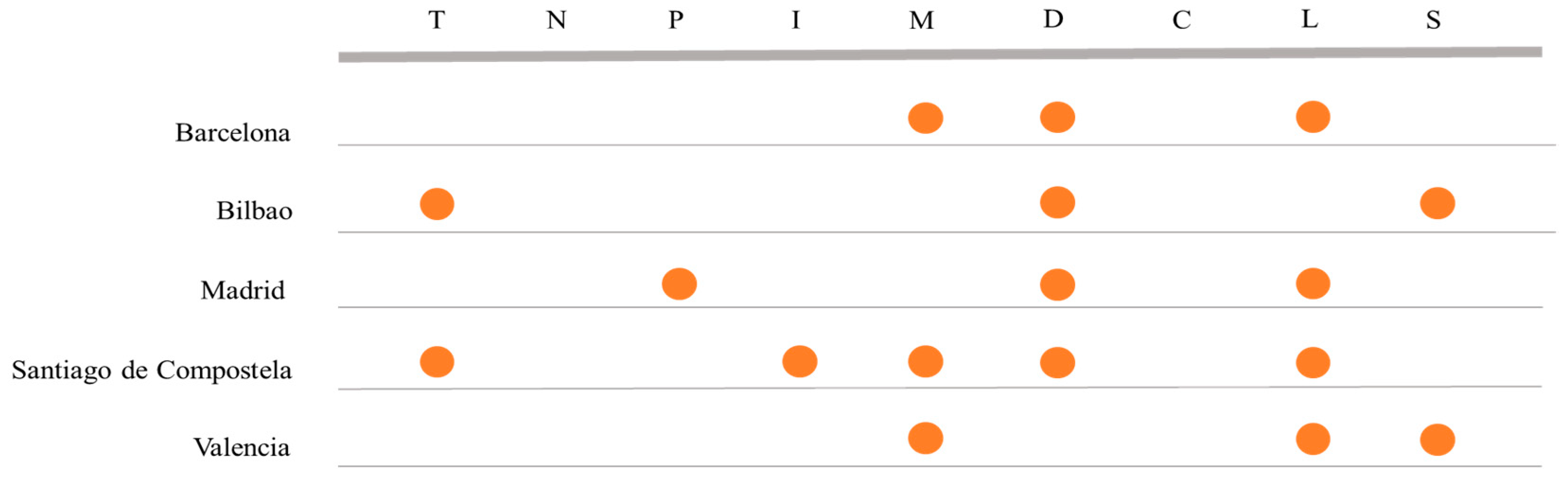
Figure 2 summarizes, for each case study, the variables selected by the corresponding model obtained.
First of all, it should be underlined that none of the generated models recognized the number of employment contracts (C) and the total number of residences (N) as significant variables in the housing price formation.
For the five metropolitan areas analyzed, the market rents and the unemployment level were almost always identified by the algorithm implemented—four times out of five—, whereas the number of mortgages appeared in three models. These phenomena confirmed the predominant influence of the income-type characteristics on the property selling prices, attested by a wide reference literature [
39,
73,
74]. The rents, in particular, are interpreted by the market as a proxy of the dividend related to the property purchase; furthermore, it should be outlined that during the period preceding the crisis (2000–2005) in Spain the ratio between housing prices and rents strongly increased compared to its historical average, as a sign of an overvaluation of the property prices [
75]: therefore, the relationship detected by the models represents a useful reference for checking any speculative housing market bubbles. In fact, it is interesting to observe that the models obtained showed different correlations between the housing selling prices and the market rents, with different lags of the effects determined by the dependent variable. In particular: for the metropolitan area of Barcelona, the lags of the functional relationships between the housing prices and the market rents were equal to four quarters (
Lt–4), through a direct functional relationship, and two quarters (
Lt–2) with an inverse functional link; for the metropolitan area of Madrid, the model showed an inverse correlation, delayed by four quarters between the market rents (
Lt–4) and the housing prices; for the metropolitan area of Santiago de Compostela, an inverse functional relationship between the housing selling prices at time
t and the market rents at time
t–6 (
Lt–6) has been detected by the respective model; for the metropolitan area of Valencia, the market rents influence the housing prices with an inverse functional relationship and a lag of five quarters (
Lt–5).
Regarding the unemployment level, the correlation with the housing prices was affected by the high rate reached by this independent variable in Spain during the current economic crisis, that led to the adoption of the labor market reform in 2012 (Royal Decree-Law No. 3/2012), in order to encourage the worker recruitment. It is not by chance that numerous Spanish studies, analyzing the psychological effects of the economic crisis, have highlighted the negative impacts in terms of anxiety and stress about the future related to a long-term unemployment period [
76]. Therefore, in the four models in which this variable appears, the unemployment level was always correlated to the housing prices through an inverse functional relationship, although with different lags: eight quarters (
Dt–8) for the metropolitan area of Barcelona, six quarters (
Dt–6) for the metropolitan area of Bilbao, no lags (
Dt) and seven quarters (
Dt–7) for the metropolitan area of Madrid, seven quarters (
Dt–7) for the metropolitan area of Santiago de Compostela.
The number of mortgages was identified by three models (Barcelona, Santiago del Compostela and Valencia) as a significant variable in the housing price formation, characterized by the following lags: eight quarters (Mt–8) for the metropolitan area of Barcelona, two quarters (Mt–2) for the metropolitan area of Santiago de Compostela, four quarters (Mt–4) for the metropolitan area of Valencia. The increase of mortgages in the last few years has determined a demand growth in properties, that led to an increase in housing prices and in the transactions of residential units. With the exception of the model for the metropolitan area of Valencia, in which the number of mortgages appeared in a single additive term and was characterized by a direct relationship with the housing prices—that is consistent with the empirical expected phenomena, in the other two models the variable is combined with other factors. In particular, for the model of the metropolitan area of Barcelona the number of mortgages and the unemployment level appeared in the same additive term, with the same lag (t–8) and the same exponent (=0.5); the inverse correlation of this term with the housing prices outlined the higher weight of the unemployment level on the property value formation. For the model of the metropolitan area of Santiago de Compostela, the number of mortgages and the number of residential transactions was in the same additive term with different lags, and the detected correlation with the housing prices was direct, as empirically expected.
It should be noted that the population was identified as a significant factor only for the metropolitan area of Madrid, i.e., the most populous of the areas analyzed. The lag detected was equal to five quarters (Pt–5), and it was characterized by a direct correlation with the housing prices.
The variable “average selling prices of buildable soils” was characterized by a consistent direct correlation with the housing prices in the model for the metropolitan area of Valencia, with a lag of four quarters (St–4): in this case, the average incidence rate, i.e., the ratio between the average soil values and the average housing prices, was the highest (=21%) among the metropolitan area analyzed. This variable was also selected by the model for the metropolitan area of Bilbao, that was characterized by the highest average housing prices: the functional relationship with the housing prices was always direct, but with a greater lag (St–7) and a lower weight, determined by the exponent “0.5”. Furthermore, in this model the number of residential transactions was related to the housing prices through a direct and contemporary functional relationship (Tt), although in this case the variable was characterized by the minimum value—in absolute terms and in percentage of the respective population among the metropolitan areas analyzed.
Finally, the number of firms was only selected in the model for the metropolitan area of Santiago de Compostela with a lag of four quarters (It–4). The direct functional correlation detected by the model among this variable and the housing prices confirmed the empirically expected phenomena.
7. Practical Use of the Models Obtained: The Empirical Forecast of the Future Market Trends
An interesting peculiarity of the models obtained through the implementation of the methodology proposed was the forecasting capacity of the housing prices in the quarters following the last historical data recorded (referred to the III quarter of the year 2017), through an empirical procedure, alternative to the impulse response functions to be implemented in a classical VAR. Since each model correlated the property prices at time
t with socio-economic variables referring to different time lags, it is possible, for each case study analyzed, to assess the future market trend through the following logical procedure: (i) the temporally nearest independent variable to time
t with the exception of the variable
Yt–1 represents the control variable, i.e., a sensitivity analysis of the property prices subsequent to the third quarter of the year 2017 is developed through constant variations of the independent variable in the future quarters, within a range of variation appropriately established; (ii) the independent variable that temporally comes before the control variable establishes the duration of the forecast period (time variable) of the housing prices.
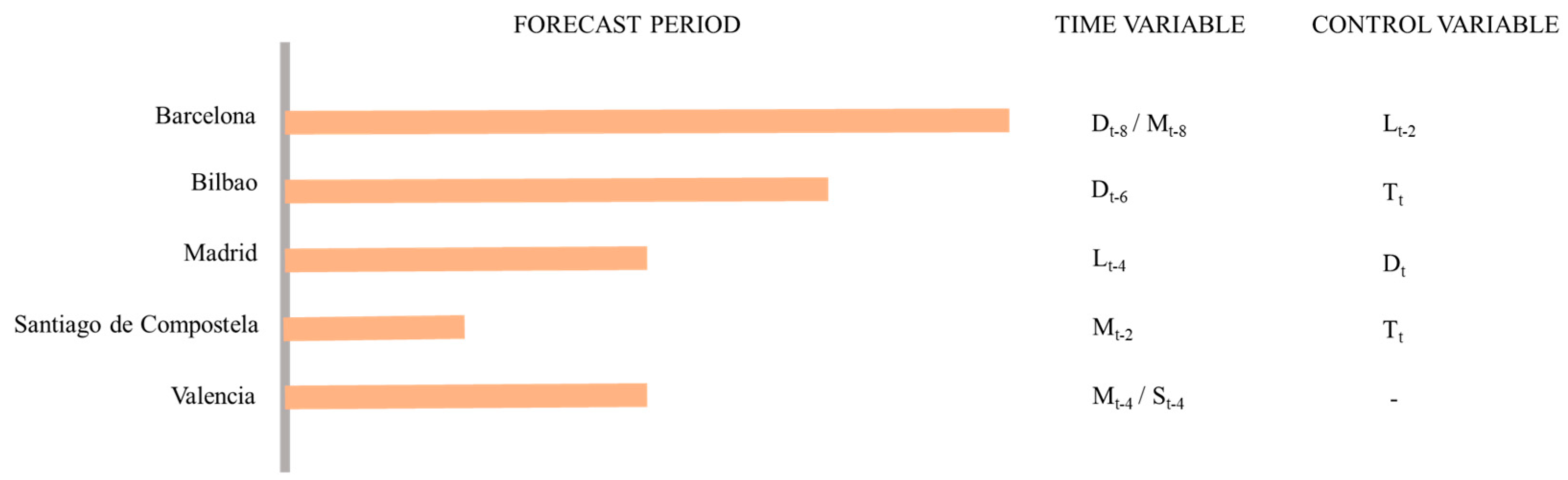
Figure 3 shows, for each of the five case studies, the forecast period for which the construction of the future market trend is obtained, the time variable and the control variable.
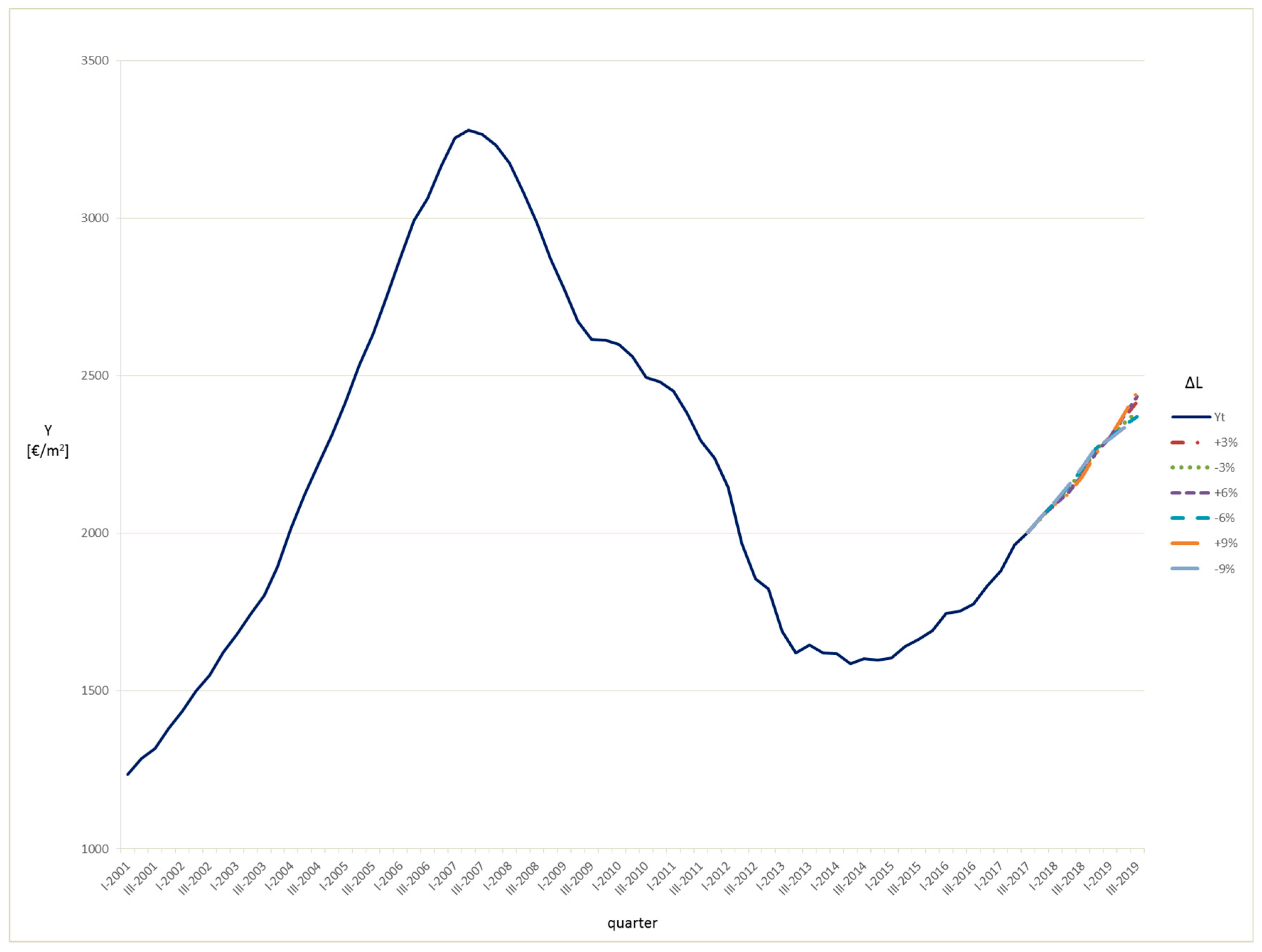
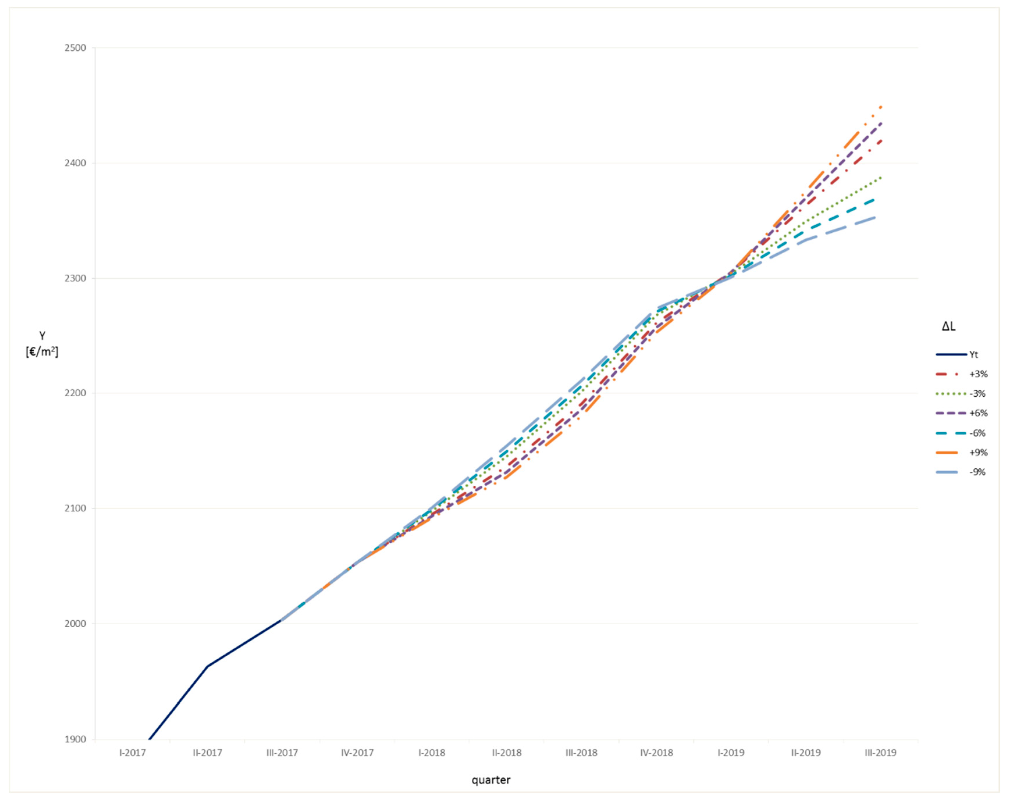
For the metropolitan area of Barcelona (
Figure 4 and
Figure 5), the housing prices after the third quarter of the year 2017 were obtained by varying the market rents in eight future quarters and considering the volatility of this factor in a range [−9%; +9%]. The graphical outputs show a positive correlation over time between the market rents and the housing selling prices: this relationship is more evident starting from the convergence point that occured in the first quarter of the year 2019, after which positive changes in the market rents determined increases in the housing prices, whereas decreasing changes in the market rents negatively affect the trends in the property prices. However, in the two years considered, the maximum housing selling price differential between a very positive trend in the market rents (+9%) and a respective very negative trend (−9%) was not very significant, being equal to about 4%. Therefore, according to the model and the possible variations considered for the market rents, in the metropolitan area of Barcelona the housing prices should increase in the following two years.
For the metropolitan area of Bilbao (
Figure 6 and
Figure 7), the housing prices after the third quarter of the year 2017 were obtained by varying the number of the residential transactions in six future quarters and, taking into account the volatility of this factor, in a range [−15%; +15%]. The trend was always increasing, except for a very high negative change in the purchase transactions (−15%), for which, starting from the second quarter of the year 2018, the property prices decreased. In the year and a half assessed, the maximum housing selling price differential between a very positive trend in the residential transactions (+15%) and a respective very negative trend (−15%) was equal to about 11%. The model developed showed that in the metropolitan area of Bilbao the housing prices should tend to grow, and even a strong reduction in the residential transactions would result in a substantially stable trend of the property prices.
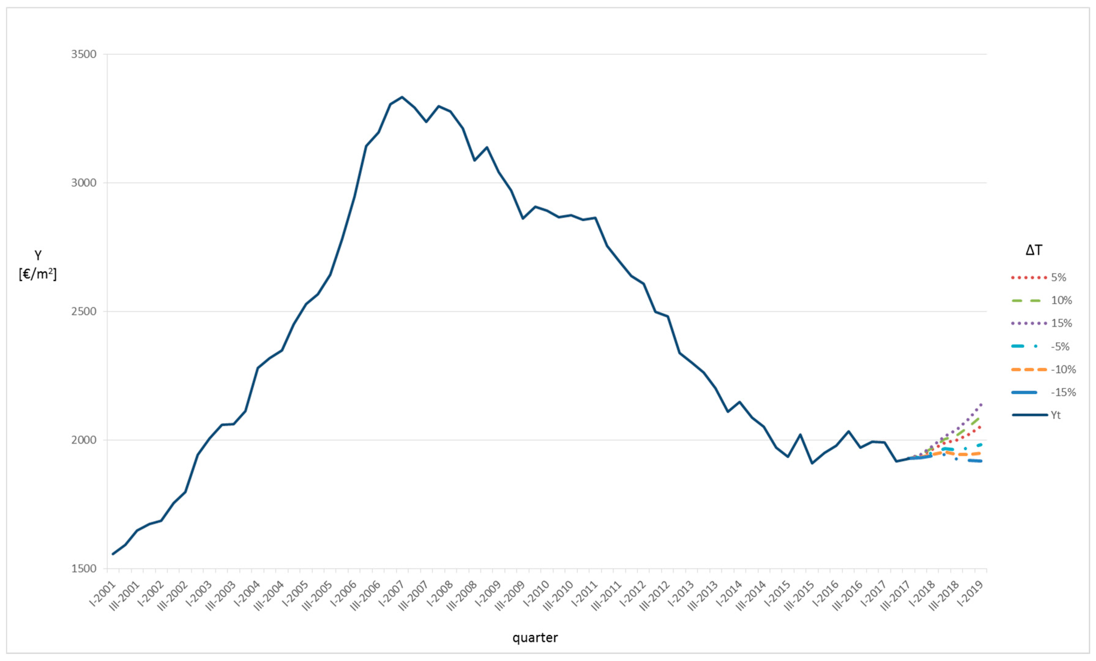
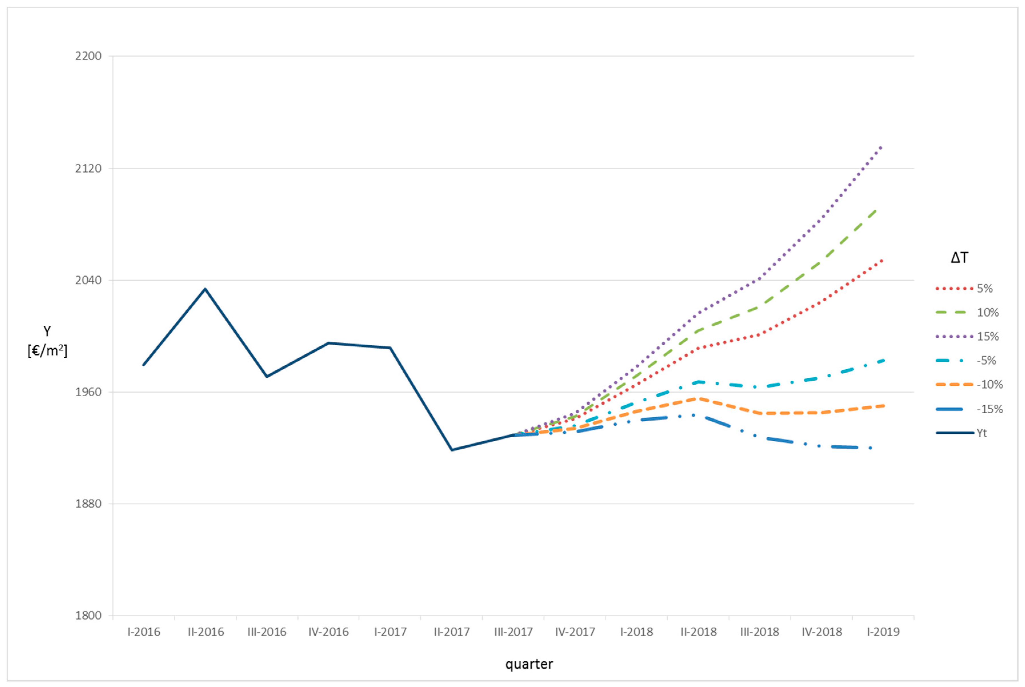
For the metropolitan area of Madrid (
Figure 8 and
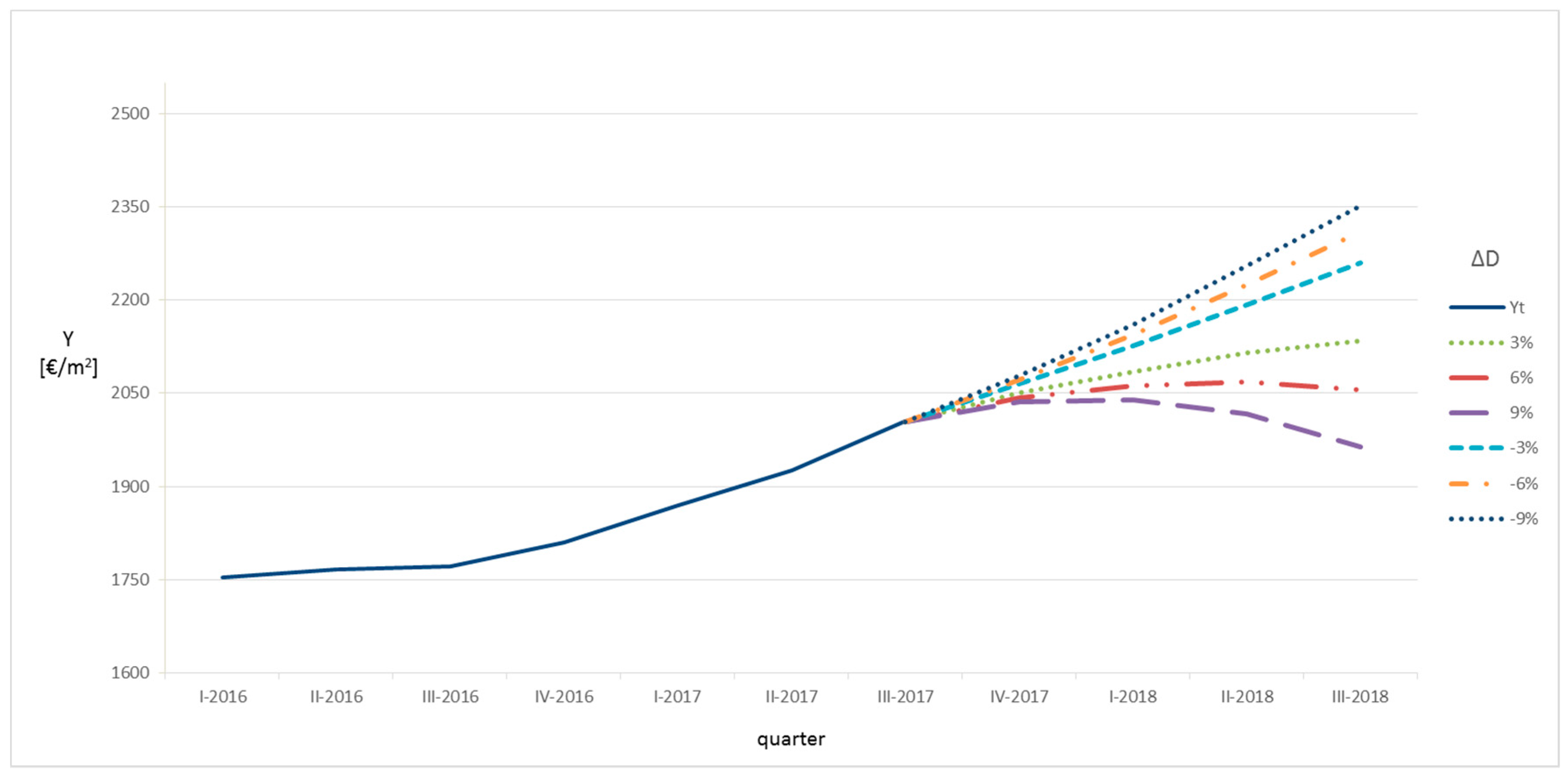
Figure 9), the future property prices were determined by varying the unemployment level in the year (four quarters) that follows the third quarter of the year 2017, in a range [−9%; +9%]. The results obtained showed a significant sensitivity of the housing selling prices to variations in the unemployment level. In particular, the maximum housing selling price differential between a substantial increase in the unemployment level (+9%) and a trend characterized by a consistent increase in new jobs (−9%) was equal to about 20%. Therefore, it is evident that a good welfare policy, that continues the social improvements activated by the labor market reform in 2012, would have significant effects on the housing market in the metropolitan area of Madrid.
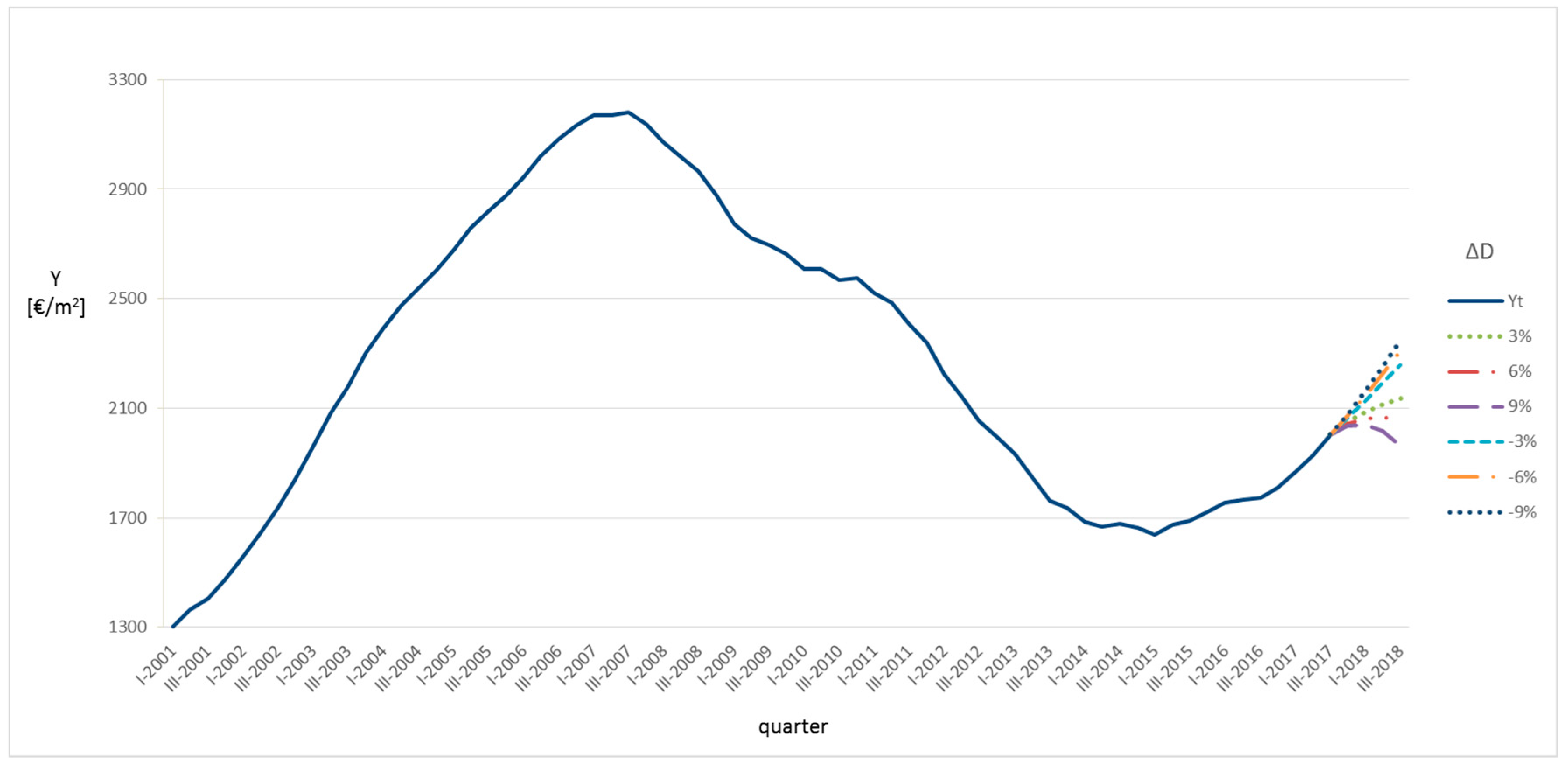
For the metropolitan area of Santiago de Compostela (
Figure 10 and
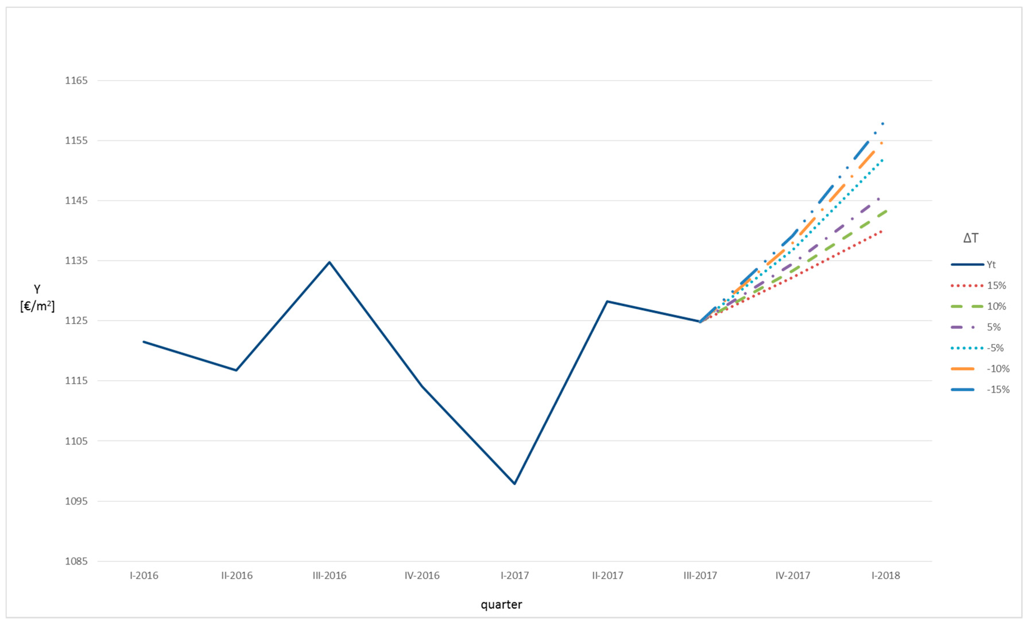
Figure 11), the future trends of the housing selling prices were obtained by changing the number of the residential transactions in the two quarters following the last reporting period (3rd quarter of the year 2017) and in a range [−15%; +15%]. It is evident that in all the forecasts the property prices tended to grow: in particular, the maximum housing selling price differential between a very positive trend in the residential transactions (+15%) and a respective very negative trend (−15%) was minimal, around 2%. Therefore, in the metropolitan area of Santiago de Compostela the housing prices tended to increase in the following two quarters.
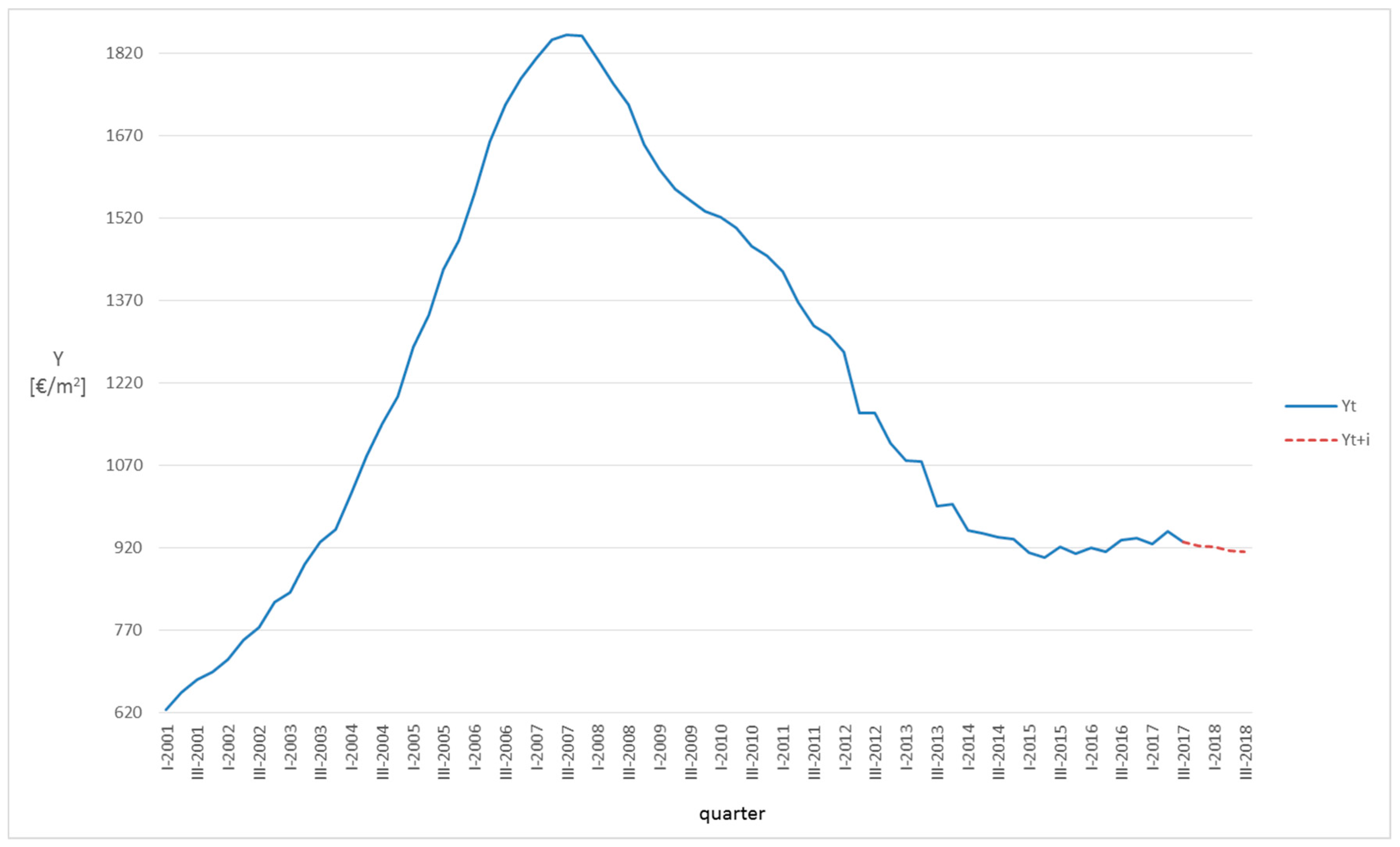
The model structure obtained for the metropolitan area of Valencia, in which the temporal correlation closest to time
t had a lag of four quarters (
St–4 and
Mt–4), allowed the construction of a single future evolution of the housing selling prices in the year following the third quarter of the year 2017 to be performed, i.e., to by-pass the definition phase of the control variable.
Figure 12 shows the property prices future trend in the year after the third quarter of the year 2017: the forecast was a rather negative housing market evolution, with an estimated decrease in the residential property prices of around −2%.
8. Conclusions
The determining role of the housing market on the global economic trends and the extreme volatility that has characterized the property values in recent years have spread the need for advanced econometric models, capable of forecasting future bubbles (and consequent bursts) and monitoring sudden scenario evolutions, in order to check the following effects.
The present research has studied the correlations between the housing prices and the main socio-economic influencing factors in five Spanish metropolitan areas. The methodology implemented is an innovative technique, that employs a genetic algorithm to identify the best functional relationships among the variables selected, and the data sample has been obtained by considering the main variables identified in the reference literature. The methodology used has allowed models of simple interpretation to be generated, characterized by both high statistical performance and compliance with the expected empirical phenomena, and to identify the best combination of the possible lags of the considered input variables in the explanation of housing prices. In this sense, the method applied represents an evolution of the classical machine learning techniques, as it allows the prediction accuracy, the interpretability and the simplicity of the models to be obtained simultaneously, by considering all the possible combinations among the variables and the respective lags, and taking into account a set of eligible exponents.
For the metropolitan areas in analysis, the results have shown different functional relationships between the housing prices and the influencing factors selected by the methodology proposed, according to the respective economic conditions that affect the property value formation. Albeit with different lags and weights, the factors that indirectly represent the population’s income capacity—market rents, unemployment level, number of mortgages—play a decisive role in the Spanish housing price explanation.
The empirical procedure applied for the construction of the future trends of the property values has highlighted the forecasting and monitoring potentialities of the models generated by the methodology. Starting from the actual available data, the procedure implemented has allowed, for each case study analyzed, a frontier more or less wide to be described, according to the volatility of the control variable of the possible evolutions of the housing prices in the future. The results have shown that: the housing prices tend to grow in the metropolitan areas of Barcelona, Bilbao and Santiago de Compostela; a slight decrease in the housing prices would be expected in the metropolitan area of Valencia; the future trend of the housing prices in the metropolitan area of Madrid strongly depends on the evolution of the corresponding unemployment level. Therefore, a good welfare policy could determine significant effects on the housing market.
Definitely, according to the analysis carried out for the five metropolitan areas considered, Barcelona, Bilbao and Santiago de Compostela constitute the most convenient territories in which the operators could invest, due to a lower risk and almost certain increases in the future property values.
The fundamental support that could derive from the implementation of the methodology proposed is essentially evident: in fact, the forecasting models could be used (i) by public entities, in order to be able to define a more transparent and lower uncertain framework in the decisional phases for welfare, monetary and/or fiscal policy interventions, and consequently to anticipate and check future housing bubbles through appropriate economic policies, (ii) by private investors, in order to optimize the management of the property assets and to identify the most attractive territorial areas for new urban development initiatives, (iii) by credit institutions, in order to have more reliable valuation tools for the assessment of the mortgage lending values of properties as securities for credit exposures, (iv) by construction companies, interested in planning the beginning of the works in order to capture the opportunities deriving from the best market conditions: among the metropolitan cities analyzed, this is the case of Madrid, where the construction companies could plan their activities on the territory in relation to the lags in property value increases determined by the model, starting from the welfare policies to be launched by the Public Administration.
Further insights may involve, when sufficient data are available, other variables (interest rate, money supply, housing stock, number of construction, etc.) and consider the possibility of simplifying the functional relationships between the housing prices and the influencing factors, through a generalization of the mathematical correlations, that could be valid for several territorial contexts, in which the market specificities should be obviously expressed through different and appropriate multiplicative coefficients of the selected variables.

 ,
, 


