Investigating a Serious Challenge in the Sustainable Development Process: Analysis of Confirmed cases of COVID-19 (New Type of Coronavirus) Through a Binary Classification Using Artificial Intelligence and Regression Analysis

Abstract

Nowadays, sustainable development is considered a key concept and solution in creating a promising and prosperous future for human societies. Nevertheless, there are some predicted and unpredicted problems that epidemic diseases are real and complex problems. Hence, in this research work, a serious challenge in the sustainable development process was investigated using the classification of confirmed cases of COVID-19 (new version of Coronavirus) as one of the epidemic diseases. Hence, binary classification modeling was used by the group method of data handling (GMDH) type of neural network as one of the artificial intelligence methods. For this purpose, the Hubei province in China was selected as a case study to construct the proposed model, and some important factors, namely maximum, minimum, and average daily temperature, the density of a city, relative humidity, and wind speed, were considered as the input dataset, and the number of confirmed cases was selected as the output dataset for 30 days. The proposed binary classification model provides higher performance capacity in predicting the confirmed cases. In addition, regression analysis has been done and the trend of confirmed cases compared with the fluctuations of daily weather parameters (wind, humidity, and average temperature). The results demonstrated that the relative humidity and maximum daily temperature had the highest impact on the confirmed cases. The relative humidity in the main case study, with an average of 77.9%, affected positively, and maximum daily temperature, with an average of 15.4 °C, affected negatively, the confirmed cases.

1. Introduction

The concept of sustainable development as a new concept, process, and undeniable fact has emerged in the policies of major governments, and plays a key role in the development of human societies [1,2,3]. Sustainable development is, generally, a combination of the three social, economic, and environmental goals in which political goals are involved. In fact, sustainable development is the advancement of the quality of all aspects of life of today’s generation without creating negative impacts on the lives of future generations. While it may seem easy to create sustainability in theory, the process of sustainable development faces many unforeseen problems and obstacles that slow down the process. One of the anticipated problems is the emergence of epidemic diseases that not only have a negative impact on the economy but also cause social problems, both of which are fundamental to sustainable development. Although this is a temporary and transient problem, it has the potential to disrupt the process, which can have years of adverse effects. The COVID-19 (a new version of Coronavirus) is one of the newest and most serious challenges facing governments, and there has not been much research into this problem [4,5,6]. Although the understanding of COVID-19 is limited, interim guidance on laboratory biosafety was introduced by the World Health Organization (WHO) [7]. Kampf et al. investigated the persistence of coronaviruses on inanimate surfaces and ways to deal with it. They found that the period of persistence is nine days for coronaviruses, and some disinfectants, such as 62%–71% ethanol, 0.5% hydrogen peroxide, or 0.1% sodium hypochlorite can be very efficient in dealing with this virus [8]. Lai et al. have evaluated the outbreak of COVID-19 and its challenges. Based on their results, they made some recommendations for the prevention of more outbreaks of the virus [9]. In another study, the role of inanimate surfaces in the outbreak of coronaviruses is investigated by Kampf. Based on the obtained results, he provided some recommendations about the impact of surface disinfection to prevent further viral spread [10]. Telles has conducted an overview of the behaviors of viruses. Some datasets were investigated, and the obtained results show that dynamic mathematical modeling was essential to predict behaviors of viruses [11]. The role of media coverage on the public was evaluated by Wen et al. Their obtained results indicated that misleading and biased media coverage could have a negative impact on individuals’ mental health [12]. Chen et al. carried out an investigation for predicting the number of confirmed cases of COVID-19. They evaluated the trend of transmission and recovery rates based upon time, and a mathematical model was proposed. The obtained results show that the proposed model had a suitable performance to predict the confirmed cases [13]. In another study, the trend of the COVID-19 outbreak was estimated in China by Li and Feng. Their results show that rapid and dynamic strategies can be useful to diminish and constrain the current crisis [14]. Chinazzi et al. evaluated the effect of travel constraints to reduce the COVID-19 outbreak. The obtained results indicated that travel restrictions are highly effective in reducing the spread of this new coronavirus [15].

It is worth mentioning that the impact of temperature on virus spread and survival show different results. There have been some investigations on the effects of environmental parameters on epidemic diseases, too. The flu virus spreads quickly in cold and dry conditions, while it is completely inactive at temperatures above 30 °C [16,17]. However, the epidemic of one type of coronavirus, MERS-CoV, was between April and August, which meant that the virus spread quickly in warm temperature, low wind speed, low relative humidity, and high ultraviolet index [18].

A review of previous studies shows that very few researchers have addressed the challenges of the COVID-19 (new version of Coronavirus) in the sustainable development process and, also, unpredictable problems and complexity of the issues require the use of highly capable approaches like artificial intelligence methods to understanding these types of issues. Hence, due to the importance of the subject, the present study investigated the feasibility of artificial intelligence in the classification of confirmed cases of COVID-19, which is a severe challenge in the sustainable development process, and it is an imperative task. In addition, statistical analysis was carried out, and the obtained results were discussed. It is worth mentioning that this type of analysis has not been used in previous research.

2. Materials and Methods

Two approaches were used in the current study, as follows:

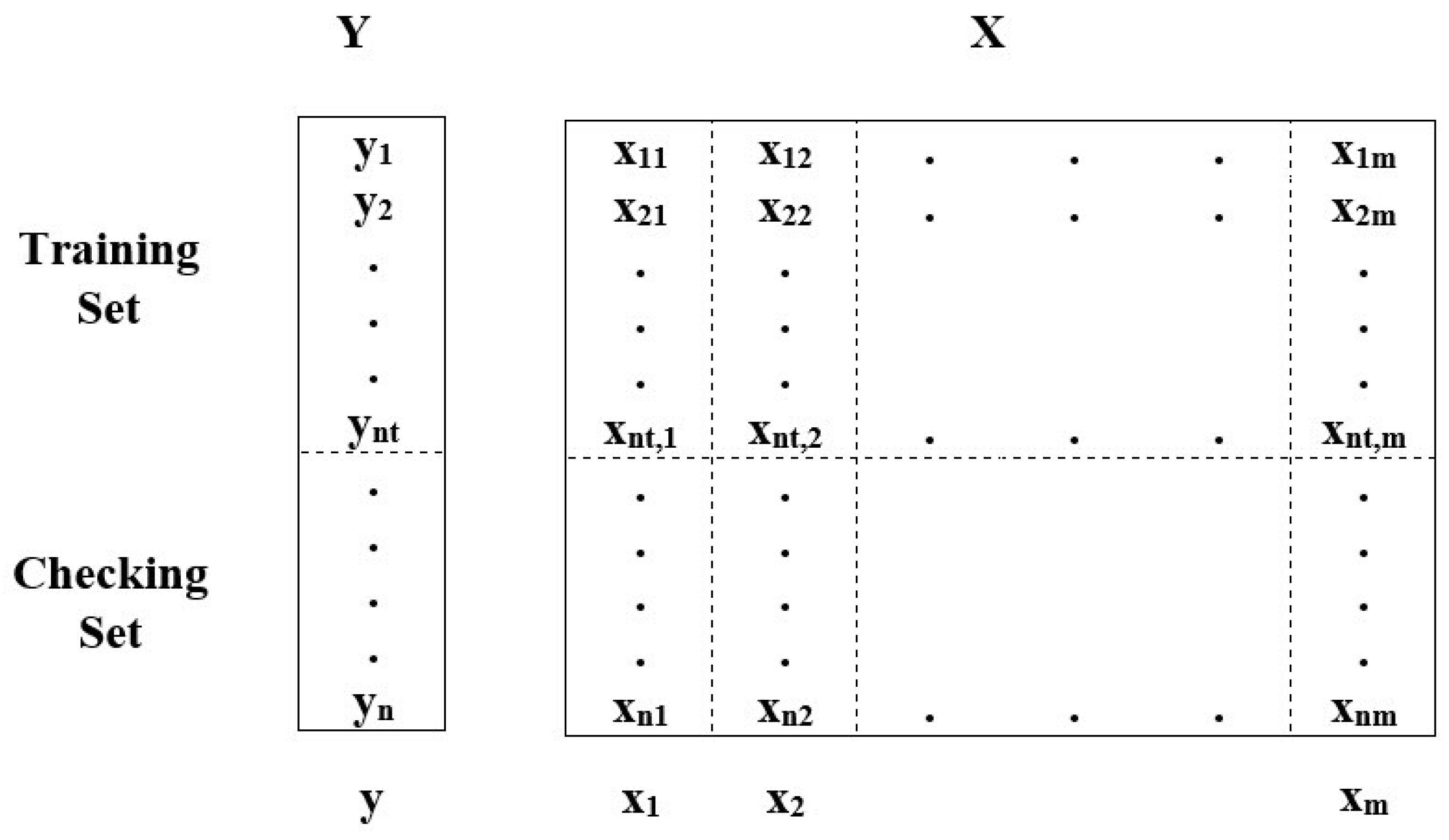
• The possible correlations among the trends of confirmed cases in different case studies were investigated, and then a binary classification model was constructed to predict and classify using the group method of data handling (GMDH) algorithm based upon some critical factors; maximum, minimum, and average temperature, the density of a city, relative humidity, and wind speed were considered as the input dataset and the number of confirmed cases was selected as the output dataset for 30 days.
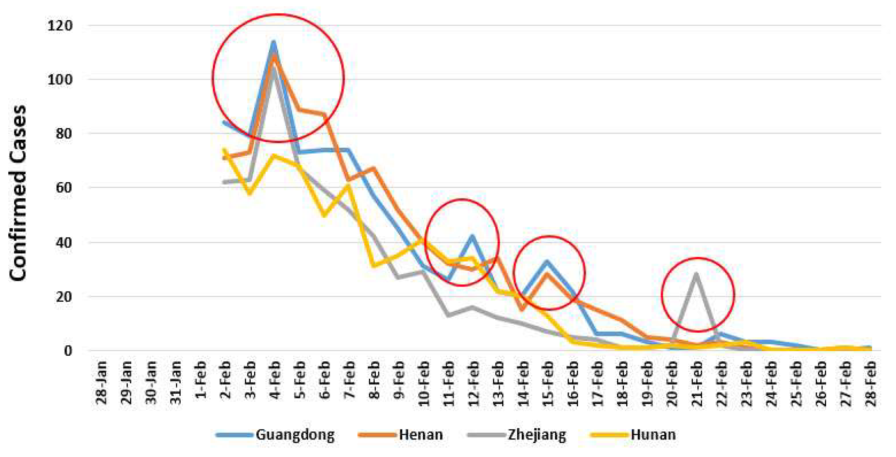
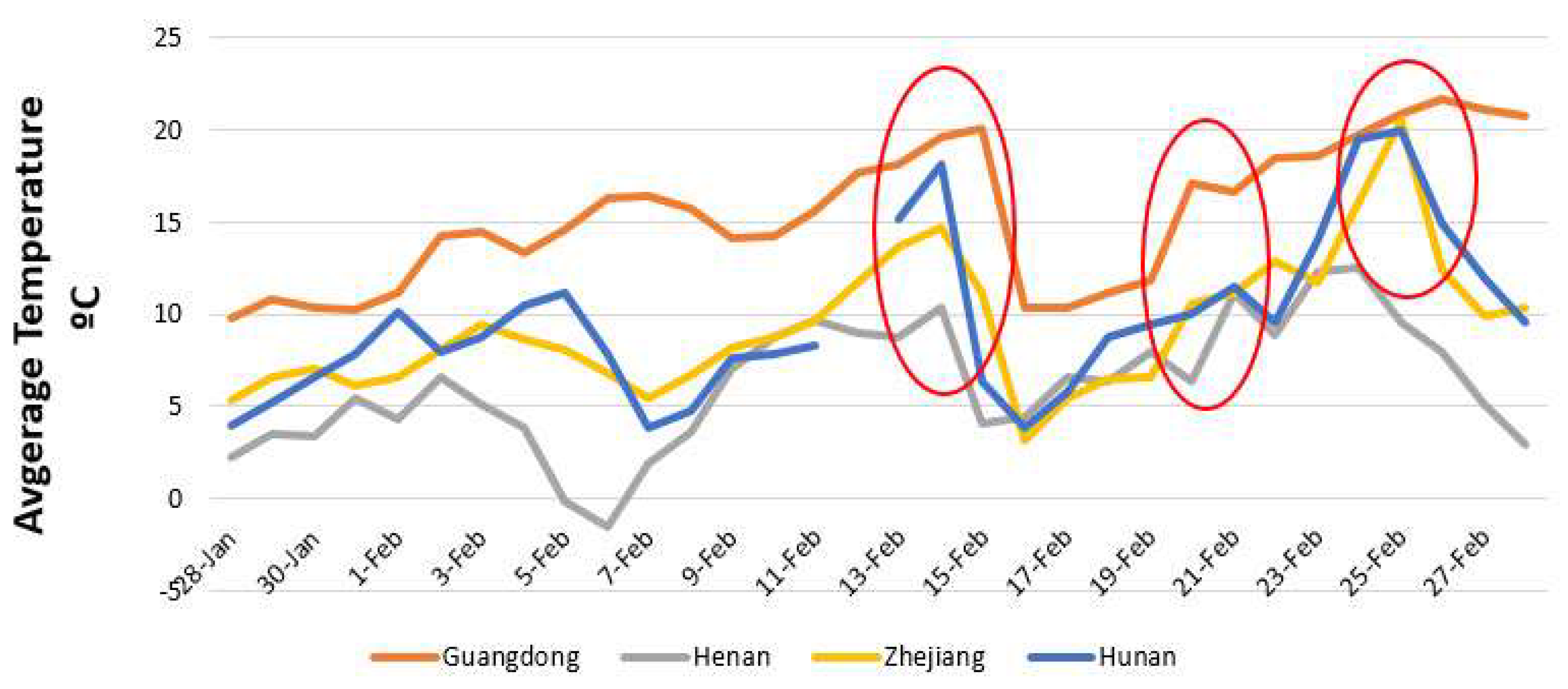
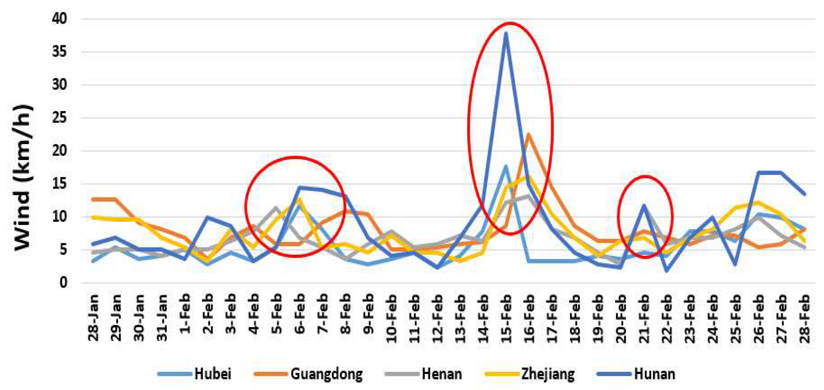
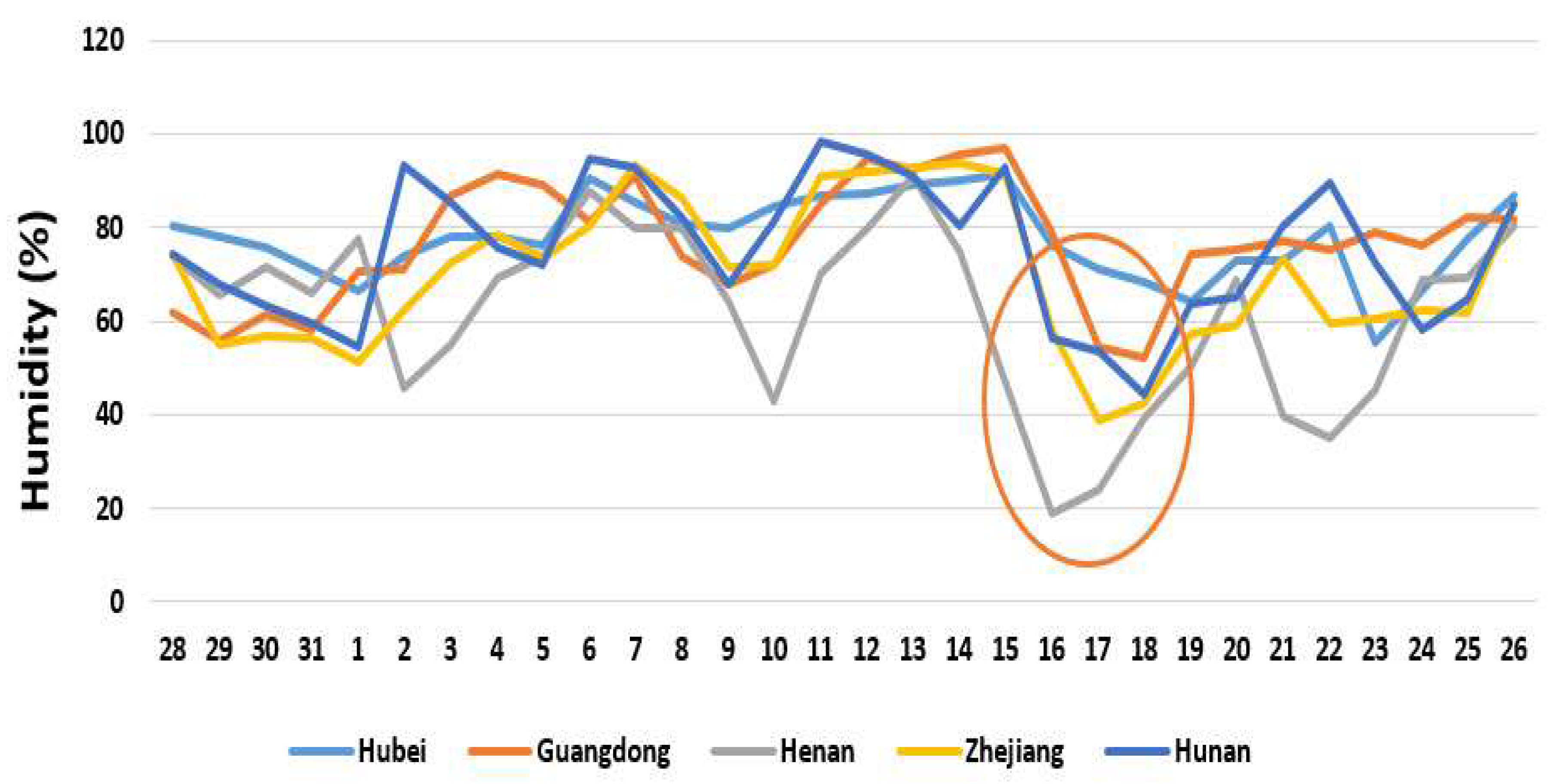
• Regression analysis was used, and a trend of the confirmed cases of COVID-19 analyzed in the five provinces with the highest confirmed cases, including Hubei, Guangdong, Henan, Zhejiang, and Hunan, and the daily fluctuations of confirmed cases were compared with fluctuations of weather parameters.

Conditions of analysis

• The environmental and urban parameters in the analysis included density, sex ratio, average age, elevation, maximum, minimum, and average temperature, relative humidity, and wind.
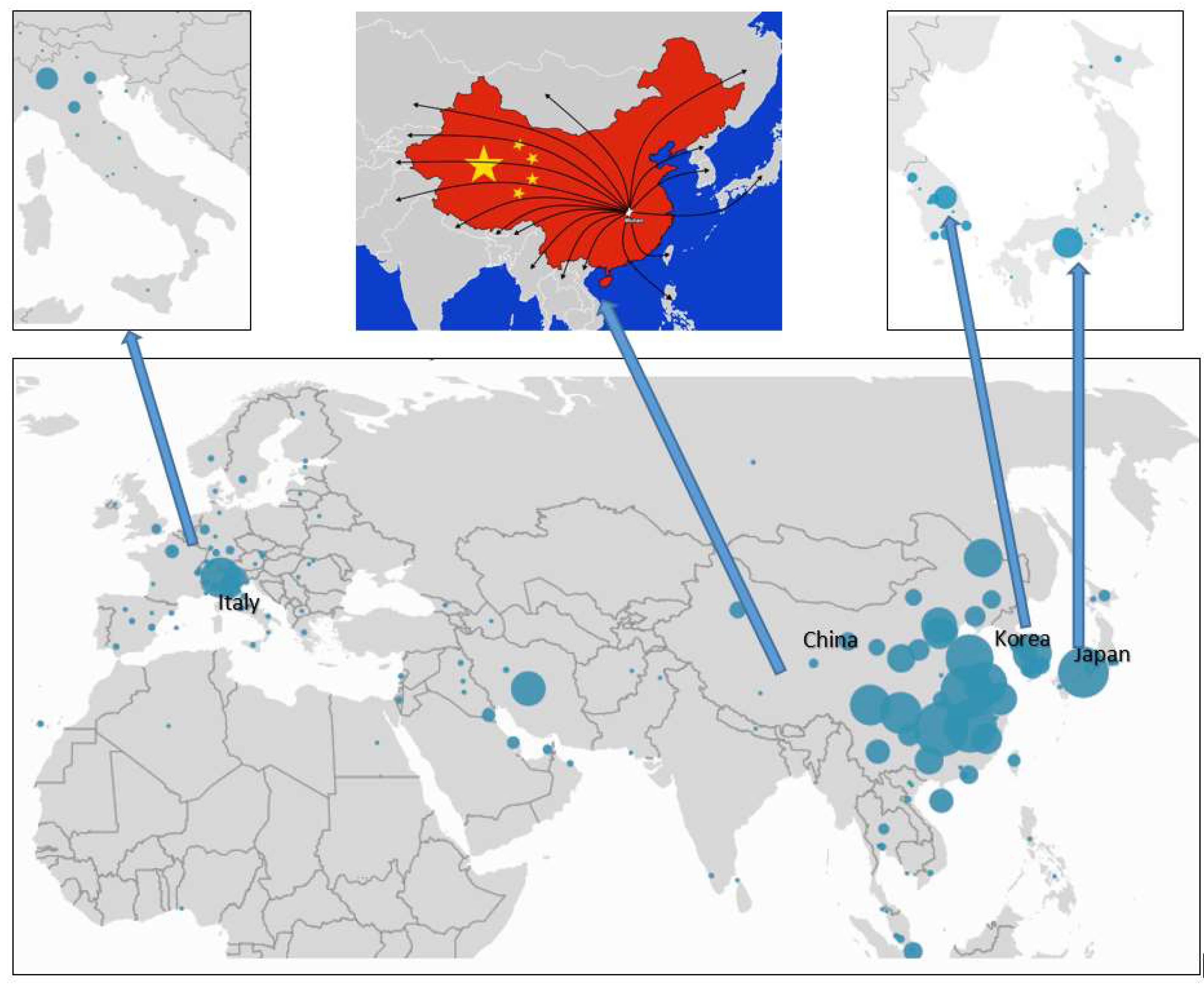
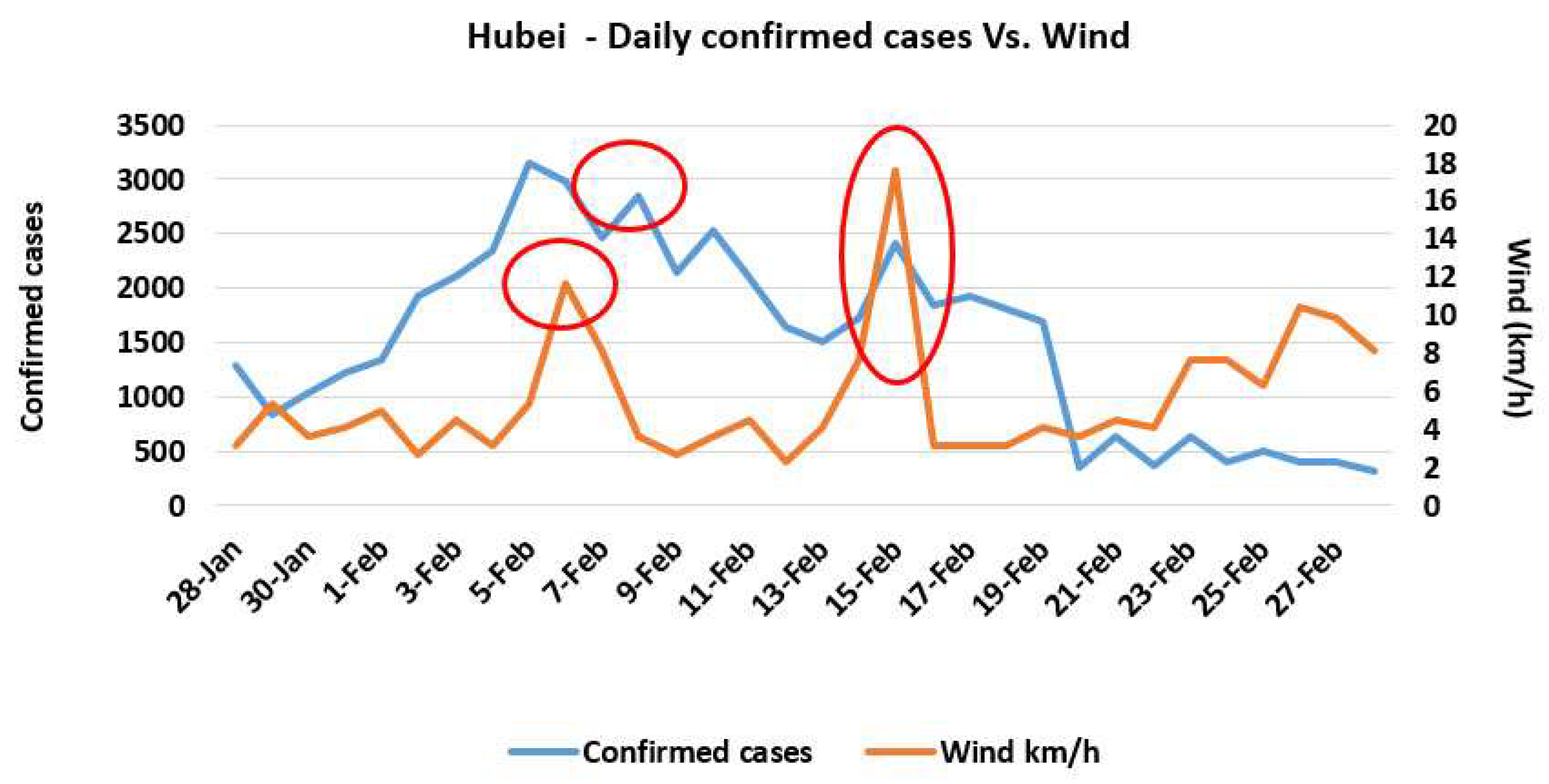
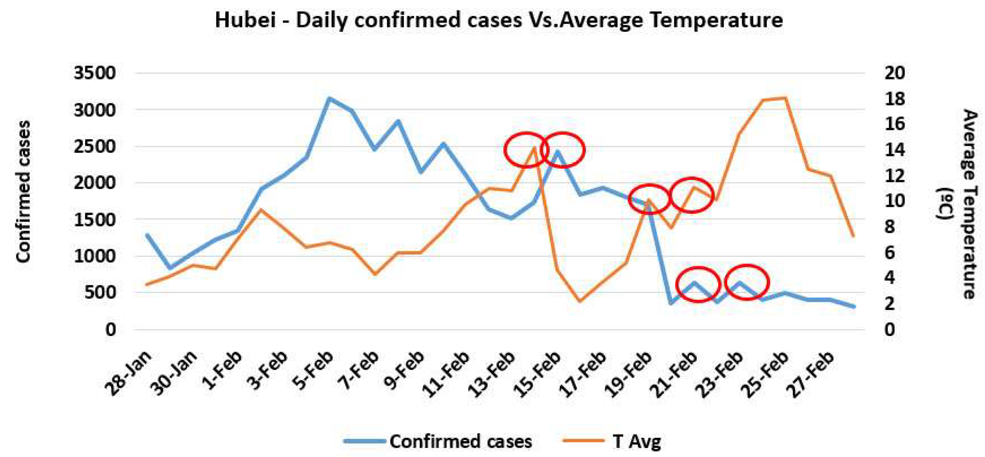
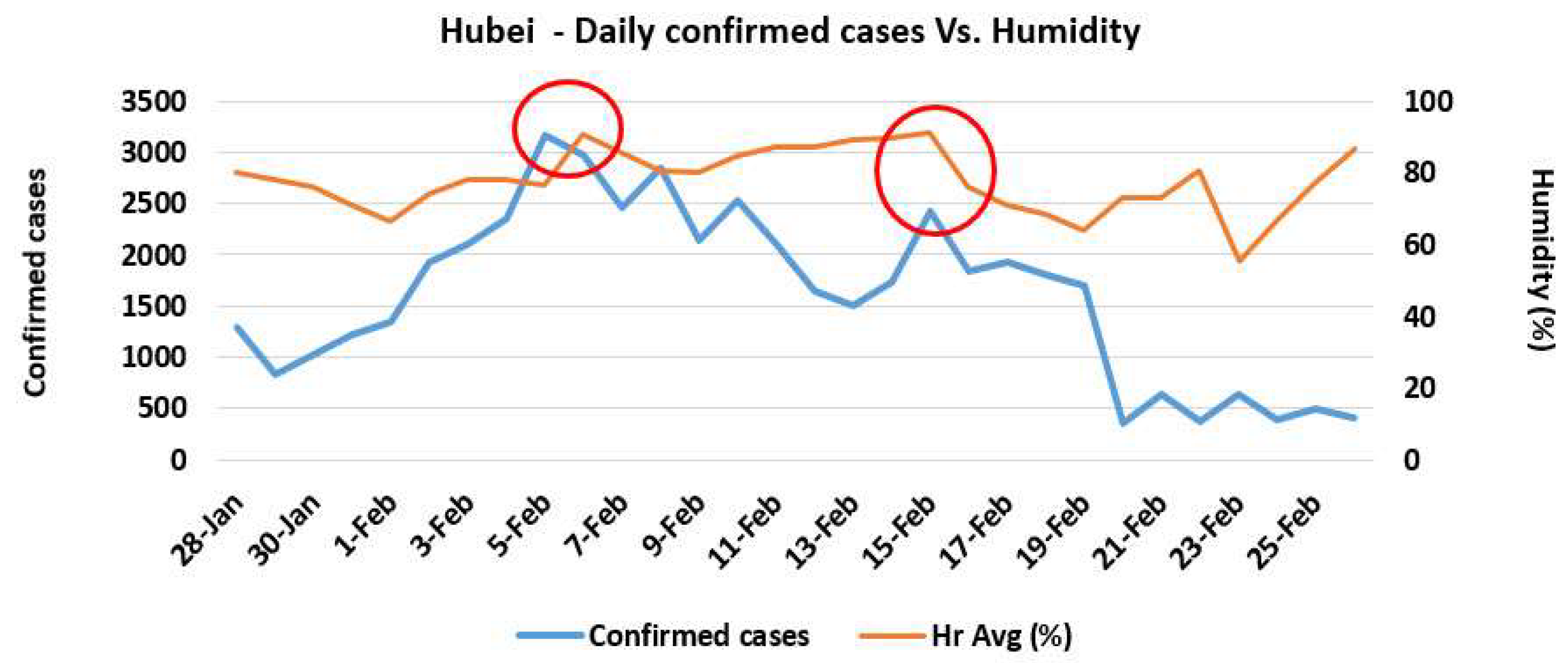
• For daily analysis of the possible trend between confirmed cases of COVID-19 and environmental factors, the data of Hubei province was used.
• The climate data is based on the stations situated in the capital of the provinces or regions because the population is generally higher in these areas.
• The analysis period was from 28 January 2020 to 26 February 2020 (30 days).
• The analysis of the possible correlations about trends of confirmed cases in different case studies was based on the average values in one month.

2.1. Case Study

To carry out the analysis of correlation among environmental factors and confirmed cases of COVID-19, a set of data, including 42 provinces in China, Japan, South Korea, and Italy, were used. The selected case studies can be seen in

Table 1. The selected case studies.

Country	Province/ Region	Capital	Population [21,22,23]	Density, Population/km2 [22,24,25,26,27,28,29,30,31,32,33]	Gender Ratio [34,35]	Average Age, years [36,37]	Elevation, m [38]
China	Hubei	Wuhan	59,170,000	318	1.06	38.4	37
	Guangdong	Canton (Guangzhou)	113,460,000	630	1.06	38.4	21
	Henan	Zhengzhou	96,050,000	575	1.06	38.4	104
	Zhejiang	Hangzhou	57,370,000	562	1.06	38.4	19
	Hunan	Changsha	68,990,000	329	1.06	38.4	63
	Anhui	Hefei	63,240,000	454	1.06	38.4	37
	Jiangxi	Nanchang	46,480,000	278	1.06	38.4	37
	Shandong	Jinan	100,470,000	653	1.06	38.4	23
	Jiangsu	Nanchino	80,510,000	785	1.06	38.4	15
	Chongqing	Chongqing	31,020,000	377	1.06	38.4	244
	Sichuan	Chengdu	83,410,000	172	1.06	38.4	500
	Heilongjiang	Harbin	37,730,000	83	1.06	38.4	126
	Beijing	Beijing	21,540,000	1313	1.06	38.4	43.5
	Shanghai	Shanghai	24,240,000	3823	1.06	38.4	4
	Hebei	Shijiazhuang	75,560,000	403	1.06	38.4	83
	Fujian	Fuzhou	39,410,000	324	1.06	38.4	14
	Guangxi	Nanning	49,260,000	209	1.06	38.4	499
	Shaanxi	Xi’an	38,640,000	247	1.06	38.4	405
	Yunnan	Kunming	48,300,000	123	1.06	38.4	1892
	Hainan	Haikou	9,340,000	275	1.06	38.4	222
	Guizhou	Guiyang	36,000,000	205	1.06	38.4	1275
	Tianjin	Tianjin	15,600,000	1380	1.06	38.4	1078
	Shanxi	Taiyuan	37,180,000	181	1.06	38.4	800
	Liaoning	Shenyang	43,590,000	299	1.06	38.4	55
	Jilin	Changchun	27,040,000	2704	1.06	38.4	202
South Korea	Seoul	Seoul	10,010,983	16541	1	43.2	38
	Daejeon	Daejeon	1,493,979	2767	1	43.2	94
	Gyeonggi	Suwon	13,653,984	1341	1	43.2	87
	South Gyeongsang	Changwon	3,438,676	326	1	43.2	2
Italy	Lazio	Rome	5,879,082	341	0.93	44.6	13
	Veneto	Venice	4,905,854	272	0.96	45.1	1
	Emilia-Romagna	Bologna	4,459,477	199	0.95	45.7	54
	Lombardy	Milan	10,060,574	422	0.94	44.8	120
Japan	Tokyo	Tokyo	13,929,286	6349	0.95	48.6	40
	Kanagawa Prefecture	Yokohama	9,058,094	3770	0.95	48.6	500
	Aichi Prefecture	Nagoya	7,552,873	1500	0.95	48.6	56
	Nara Prefecture	Nara	1,348,930	365	0.95	48.6	56.4
	Kansai region	Kyoto	22,757,897	690	0.95	48.6	50
	Tokushima Prefecture	Tokushima	728,633	180	0.95	48.6	11

and are based on the most confirmed cases of COVID-19 and available data, as shown in Figure 1. It is worth mentioning that the quarantine on travel in and out of Wuhan and the suspension of flights, trains, public buses, and the metro system began on 23 January 2020 and also on 24 January 2020 in 15 cities in Hubei [19,20]. The estimated incubation period of COVID-19 is about 2–14 days [20].

2.2. Group Method of Data Handling (GMDH)

Artificial Intelligence includes a wide range of methods and algorithms that work based on machine intelligence and has many applications in various fields of science [40], including fuzzy logic theory and application [41,42,43,44,45,46], artificial intelligence techniques and sociology [47,48,49], risk assessment and hazard identification [50,51], machine learning [52,53,54,55,56,57], and meta-heuristic algorithms and clustering techniques [58,59,60,61,62]. The group method of data handling (GMDH) type of neural network is one of these algorithms that was proposed by Ivakhnenko [63]. GMDH is a self-organization algorithm that has been used successfully for pattern recognition, optimization of complex systems modeling, and prediction problems, and it is also called the polynomial of the Ivakhnenko equation [63,64]. This algorithm can predict the value of ${\widehat{y}}_i$ from an approximate function ($\stackrel{\wedge }{f}$), for each input vector (X), which is shown in Equation (1). The basic form of a relation between input and output data can be declared as a discrete type of the Volterra functional series, referred to as the Kolmogorov–Gabor polynomial. Equation (2) shows the underlying neural network map, which is also called the polynomial of Ivakhnenko [65,66].

$$\begin{array}{l}\stackrel{\wedge }{y}=\stackrel{\wedge }{f}(x_{i1},x_{i2},x_{i3} ,\dots \dots \dots x_{im})\\ i=(1,2,3,\dots \dots ,m)\end{array}$$

(1)

$$y=a+{\displaystyle \sum _{i=1}^m{b}_i}{x}_i+{\displaystyle \sum _{i=1}^m{\displaystyle \sum _{j=1}^m{c}_{ij}}{x}_i{x}_j+}{\displaystyle \sum _{i=1}^m{\displaystyle \sum _{j=1}^m{\displaystyle \sum _{k=1}^m{d}_{ijk}}{x}_i{x}_j{x}_k+}}{\displaystyle \sum _{i=1}^m{\displaystyle \sum _{j=1}^m{\displaystyle \sum _{k=1}^m{\displaystyle \sum _{l=1}^m{e}_{ijkl}}{x}_i{x}_j{x}_k{x}_l,\dots \dots \dots \dots }}}$$

(2)

where Y is the output, m is the number of data, and X₁, X₂, X₃… X_m is the input variables vector. In many cases, the quadratic and bivariate form of this polynomial is used as Equation (3).

$$\widehat{y}=G(x_i,x_j)=a_0+a_1{x}_i+a_2{x}_j+a_3{x}_i{x}_j+a_4{x}^2{}_i+a_5{x}^2{}_j$$

(3)

Figure 2 shows a schematic of input and output variables of the GMDH algorithm, where X= (X₁, X₂, X₃, …. X_m) is the input dataset and Y= (y₁, y₂, y₃,…. y_n) is the output dataset. In this algorithm, the input dataset is imported to the initial layer and then, after evaluation and optimization, the output is considered as a new input for the next layer. This process is continued and stopped if the algorithm reaches a better answer from layer (n+1) in comparison with layer (n). As mentioned before, to deal with unpredicted and uncertain problems, the GMDH algorithm can be applied as a powerful tool. Hence, a binary classification analysis was done by the GMDH algorithm in the present study [67,68,69].

3. Results

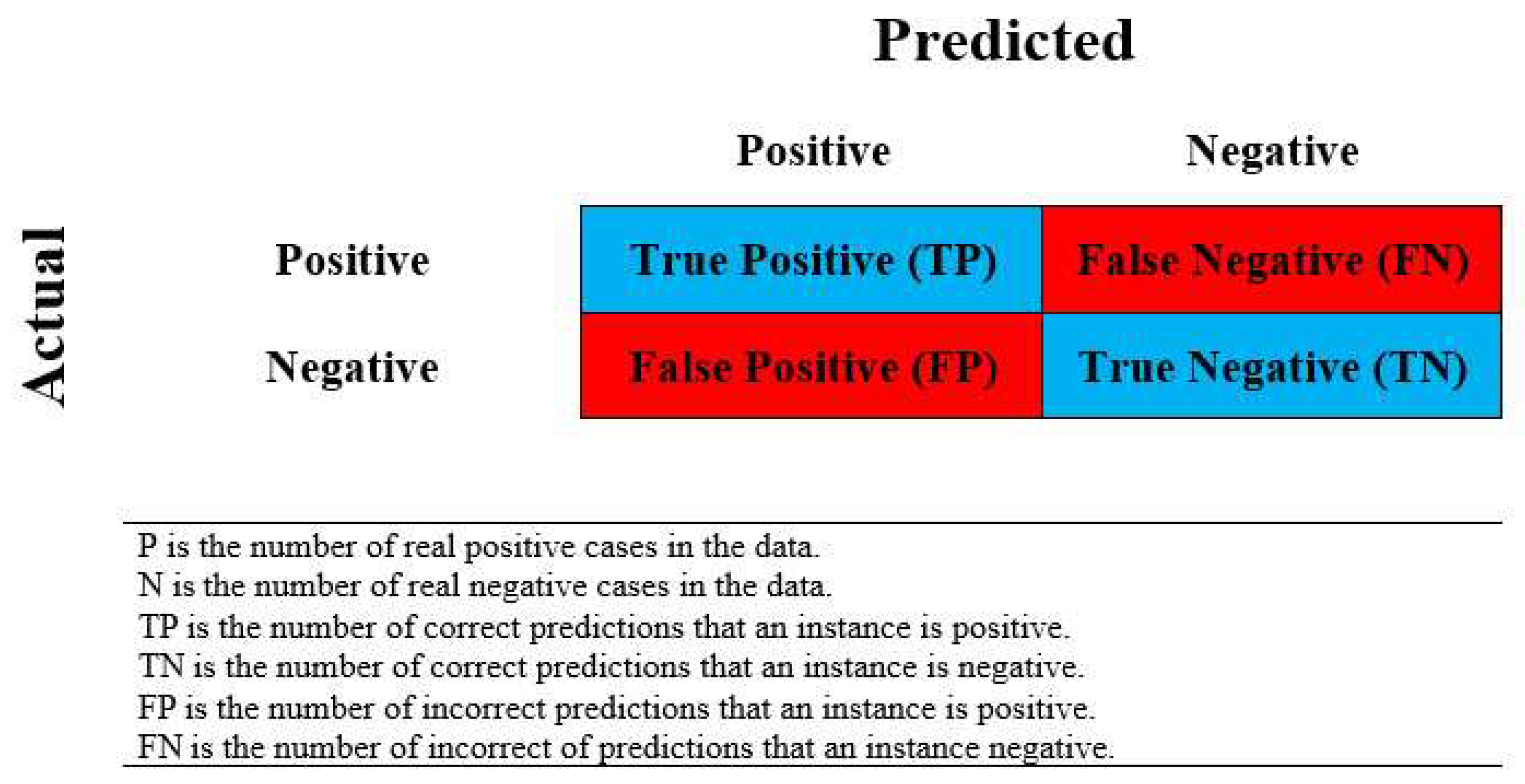
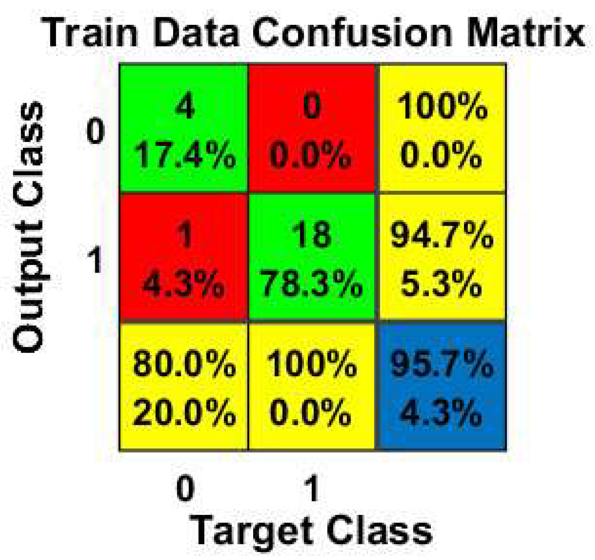
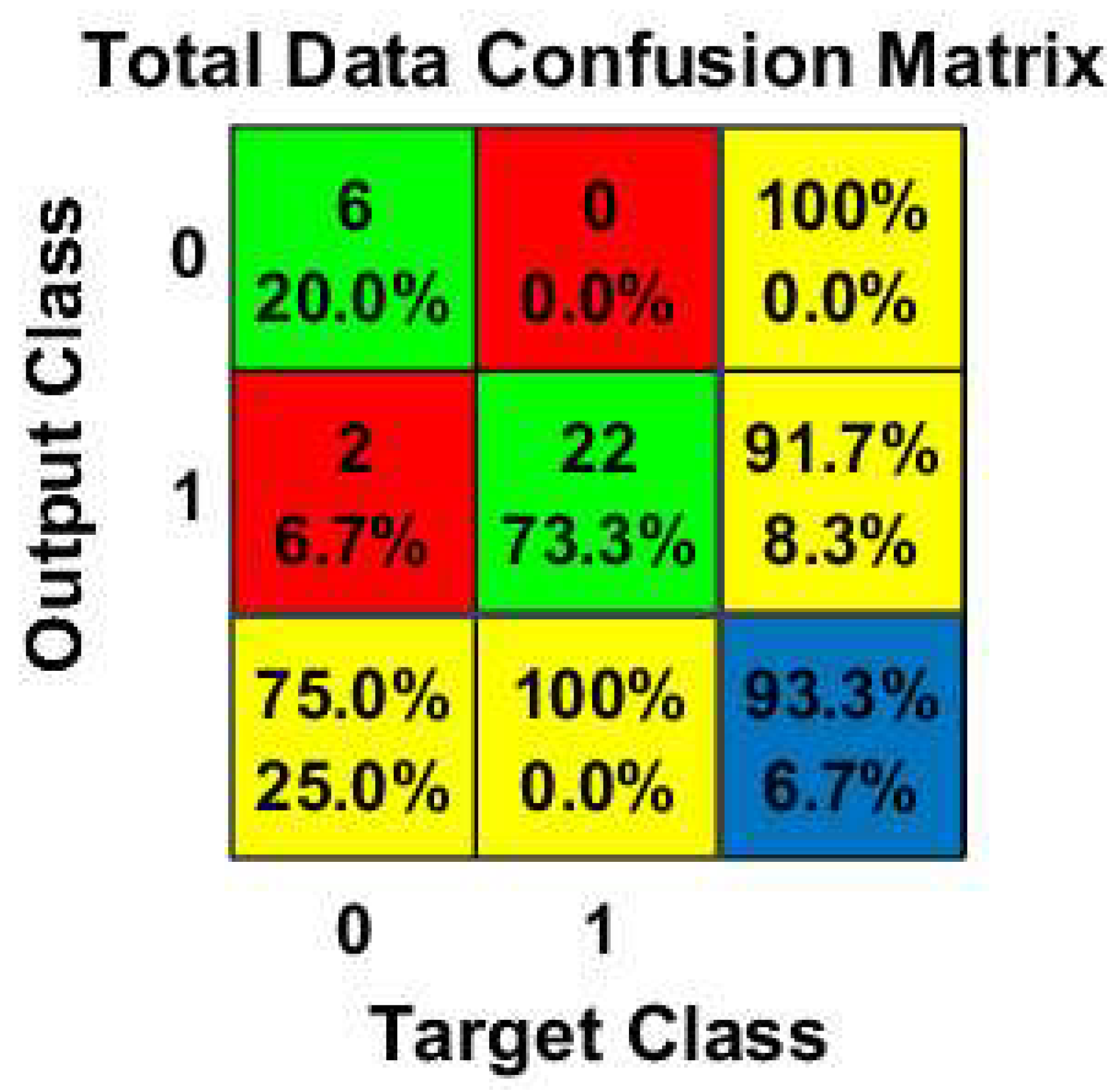
3.1. Binary Classification Modelling Using GMDH

Before binary classification modeling using the Gmdh algorithm, a regression analysis was conducted among the total data set (See

Table A1. The weather data in the case studies, [19,20,39,79,80,81,82,83,84,85,86,87,88,89].

Country	Province	Properties							February, 2020			COVID-19
		Population	Density, Population/km2	Gender Ratio	Average Age	Elevation, m	Max T °C	Min T °C	Average Temperature °C	Humidity %	Wind km/h	Confirmed Cases	Deaths
China	Hubei	59,170,000	318	1.06	38.4	37	15.4	1.4	8.3	77.9	5.4	64786	2563
	Guangdong	113,460,000	630	1.06	38.4	21	21.0	10.3	15.1	76.8	8.2	1347	7
	Henan	96,050,000	575	1.06	38.4	104	13.7	−0.1	6.3	61.9	6.8	1271	19
	Zhejiang	57,370,000	562	1.06	38.4	19	15.1	4.5	9.3	70.1	7.6	1205	1
	Hunan	68,990,000	329	1.06	38.4	63	16.2	4.4	9.6	75.2	8.4	1016	4
	Anhui	63,240,000	454	1.06	38.4	37	14.4	0.1	7.1	76.9	9.6	989	6
	Jiangxi	46,480,000	278	1.06	38.4	37	16.6	5.9	10.5	73.4	5.3	934	1
	Shandong	100,470,000	653	1.06	38.4	23	11.6	0.2	5.4	56.0	8.3	755	6
	Jiangsu	80,510,000	785	1.06	38.4	15	14.2	2.4	7.8	73.0	9.0	631	0
	Chongqing	31,020,000	377	1.06	38.4	244	14.3	8.0	10.7	78.3	3.4	576	6
	Sichuan	83,410,000	172	1.06	38.4	500	14.9	5.4	9.75	65.50	6.10	529	3
	Heilongjiang	37,730,000	83	1.06	38.4	126	−5.8	−20.6	−12.7	69.9	9.9	480	12
	Beijing	21,540,000	1313	1.06	38.4	43.5	7.8	−4.8	1.0	55.7	7.2	400	4
	Shanghai	24,240,000	3823	1.06	38.4	4	14.1	2.4	8.1	72.8	9.1	335	3
	Hebei	75,560,000	403	1.06	38.4	83	10.6	−1.5	4.1	54.6	8.5	311	6
	Fujian	39,410,000	324	1.06	38.4	14	18.4	8.3	12.7	70.6	7.4	294	1
	Guangxi	49,260,000	209	1.06	38.4	499	20.4	11.5	15.5	74.4	9.6	252	2
	Shaanxi	38,640,000	247	1.06	38.4	405	14.5	2.3	7.8	62.4	3.9	245	1
	Yunnan	48,300,000	123	1.06	38.4	1892	18.0	3.4	10.6	64.1	9.0	174	2
	Hainan	9,340,000	275	1.06	38.4	222	24.5	16.8	19.9	81.1	11.3	168	5
	Guizhou	36,000,000	205	1.06	38.4	1275	12.5	3.9	7.6	82.0	8.5	146	2
	Tianjin	15,600,000	1380	1.06	38.4	1078	8.6	−4.0	1.8	61.8	9.3	135	3
	Shanxi	37,180,000	181	1.06	38.4	800	10.0	−7.1	0.6	52.6	7.0	133	0
	Liaoning	43,590,000	299	1.06	38.4	55	2.0	−12.6	−5.36	64.22	8.26	121	1
	Jilin	27,040,000	2704	1.06	38.4	202	−2.4	−15.7	−8.96	66.52	9.60	93	1
South Korea	Seoul	10,010,983	16541	1	43.2	38	7.2	−1.1	2.6	56.1	9.1	4	0
	Daejeon	1,493,979	2767	1	43.2	94	9.2	−0.8	3.6	67.3	5.1	49	0
	Gyeonggi	13,653,984	1341	1	43.2	87	7.4	−1.8	2.5	79.3	7.1	2	0
	South Gyeongsang	3,438,676	326	1	43.2	2	12.0	4.5	8.0	67.0	10.3	922	10
Italy	Lazio	5,879,082	341	0.93	44.6	13	15.9	6.5	11	71	9	3	0
	Veneto	4,905,854	272	0.96	45.1	1	11.3	3.1	7	83	7	42	1
	Emilia−Romagna	4,459,477	199	0.95	45.7	54	14.5	3.1	8	72	7	23	0
	Lombardy	10,060,574	422	0.94	44.8	120	15.2	0.1	7	69	8	240	9
Japan	Tokyo	13,929,286	6349	0.95	48.6	40	13.5	4.3	8	58	10	14	0
	Kanagawa Prefecture	9,058,094	3770	0.95	48.6	500	13.3	5.5	9.1	56.3	13.9	1	0
	Aichi Prefecture	7,552,873	1500	0.95	48.6	56	12.1	3.6	7	65	12	2	0
	Nara Prefecture	1,348,930	365	0.95	48.6	56.4	11.6	2.9	6.6	71.5	7.7	1	0
	Kansai region	22,757,897	690	0.95	48.6	50	11.8	3.8	7.2	68.3	7.5	1	0
	Tokushima Prefecture	728,633	180	0.95	48.6	11	12.6	5.2	8.59	64.02	11.94	831	5

in Appendix A) for 42 case studies in four countries, including China, Japan, South Korea, and Italy. This analysis shows that there is a low correlation coefficient (R²); hence, it can be concluded that we should evaluate case by case for binary classification modeling, and Hubei province in China was selected as a case study for this part of the analysis.

Initially, evaluating the parametric correlation of each independent input dataset is necessary for carrying out reliable modeling [70,71,72,73]. Hence, before modeling, a correlation analysis was conducted using Pearson’s correlation coefficient among the dataset for five independent input data, including maximum, minimum, and average temperature, relative humidity, and wind speed. Furthermore, it should be noted that independent input data, including the density of the city, is not considered for evaluating the parametric correlation because the value of this parameter is constant. The mathematical relations of Pearson’s method can be expressed in Equations (4)–(7) [74].

$$\rho =r=\frac{S{P}_{Dxy}}{\sqrt{S{S}_X.S{S}_Y}}$$

(4)

$$S{P}_{Dxy}={\displaystyle \sum xy-\frac{({\displaystyle \sum x})({\displaystyle \sum y})}{n}}$$

(5)

$$S{S}_X={\displaystyle \sum _i^n{x}_i^2}-\frac{{({\displaystyle \sum x_i})}^2}{n}$$

(6)

$$S{S}_Y={\displaystyle \sum _i^n{y}_i^2}-\frac{{({\displaystyle \sum y_i})}^2}{n}$$

(7)

where $\rho$ is the Pearson’s correlation coefficient for two independent parameters that are shown with X and Y, and $S{P}_{Dxy}$ is the covariance between them. The standard deviation of X and Y are indicated with $S{S}_X$ and $S{S}_Y$.

Table 2. The correlation coefficient between five environmental factors.

Environmental Factors	Maximum Temperature °C	Minimum Temperature °C	Average Temperature °C	Relative Humidity %	Wind Speed km/h
Maximum Temperature	1	0.63	0.83	−0.11	0.35
Minimum Temperature	0.63	1	0.78	0.24	0.28
Average Temperature	0.83	0.78	1	−0.14	0.15
Relative Humidity	−0.11	0.24	−0.14	1	0.33
Wind Speed	0.35	0.28	0.15	0.33	1

shows the results of the correlation coefficient analysis for five independent input data. According to the previous studies, when $\left|\rho \right|\rangle 0.8$, the correlation coefficient is strong, hence the obtained results show that independent input data were correctly selected. Although there is a correlation coefficient of 0.83 between the maximum and average temperatures, it can be accepted because this value is very insignificant.

Secondly, determining the control parameters of the algorithm is an important task because it plays a key role in the fast convergence of the algorithm. There are no specific relations about most of these parameters, and they are determined based upon previous studies, experts, and trial and error. Hence, the selection pressure is dimensionless and has an impact on the sensitivity of the modeling error [75]. It is selected as 0.6 based upon the most recent studies. However, the maximum number of layers and the maximum number of neurons in a layer are considered based upon expert opinions and trial and error [76]. For this purpose, a range of values was determined for the maximum number of layers equal to 5, 10, and 15, and also another range of values was considered including 5, 10, 15, 20, and 30. It is worth mentioning that the confusion matrix is used as the measure of accuracy to evaluate the performances of the binary classification model by the GMDH algorithm. The basic form of a confusion matrix is shown in Figure 3, and Equations (8) and (9) indicate the mathematical relations of accuracy and error.

$$Acc=\frac{TP+TN}{TP+FP+TN+FN}$$

(8)

$$Error=\frac{TP+TN}{TP+FP+TN+FN}=1-Acc$$

(9)

According to the maximum number of layers and the maximum number of neurons in a layer, in total, 20 models were constructed. The six notable factors, namely the maximum, minimum, and average temperature, the density of cities, relative humidity, and wind speed were considered as the input dataset and the number of confirmed cases was chosen as the output dataset for 30 days. It should be noted that the two classes (label) are assigned and considered for the number of confirmed cases, and this means that, for the number of confirmed cases under 850, people were given label “0” and, for the number of confirmed cases above 850, people were given label “1”. In addition, there is the information of Wuhan city for 30 days as the number of cases studies; for modeling, 75% of cases were considered as training cases and the rest were considered as testing cases [77]. The obtained results of the accuracy of the training and testing models are shown in

Table 3. The accuracy of the GMDH algorithm to classify days based upon confirmed cases.

Models No.	SP	Maximum Number of Layers	Maximum Number of Neurons in a Layer	Accuracy of Training (%)	Accuracy of Testing (%)
1	0.6	5	5	73.9	71.4
2	0.6	5	10	91.3	71.4
3	0.6	5	15	95.7	85.7
4	0.6	5	20	80.5	42.9
5	0.6	5	25	91.3	71.4
6	0.6	10	5	95.7	71.4
7	0.6	10	10	73.9	71.4
8	0.6	10	15	82.6	71.4
9	0.6	10	20	95.7	57.1
10	0.6	10	25	87	71.4
11	0.6	15	5	82.6	71.4
12	0.6	15	10	91.3	71.4
13	0.6	15	15	87	71.4
14	0.6	15	20	91.3	71.4
15	0.6	15	25	87	85.7
16	0.6	20	5	91.3	85.7
17	0.6	20	10	95.7	42.9
18	0.6	20	15	91.3	42.9
19	0.6	20	20	82.6	85.7
20	0.6	20	25	95.7	71.4

.

After modeling, a simple ranking was conducted for determining the best model based on the study of Zorlu et al. [78]. The results of this ranking have been shown in

Table 4. The Ranking of binary classification models.

Models No.	SP	Maximum Number of Layers	Maximum Number of Neurons in a Layer	Ranking for Accuracy of Training	Ranking for Accuracy of Testing	Total Rank
1	0.6	5	5	15	19	34
2	0.6	5	10	19	19	38
3	0.6	5	15	20	20	40
4	0.6	5	20	16	18	33
5	0.6	5	25	19	19	38
6	0.6	10	5	20	19	39
7	0.6	10	10	15	19	34
8	0.6	10	15	17	19	36
9	0.6	10	20	20	18	38
10	0.6	10	25	18	19	37
11	0.6	15	5	17	19	36
12	0.6	15	10	19	19	38
13	0.6	15	15	18	19	37
14	0.6	15	20	19	19	38
15	0.6	15	25	18	20	38
16	0.6	20	5	19	20	39
17	0.6	20	10	20	17	37
18	0.6	20	15	19	17	36
19	0.6	20	20	17	20	37
20	0.6	20	25	20	19	39

.

The obtained results from Table 4 indicate that the 3rd model has highly acceptable degrees of accuracy and robustness. Figure 4, Figure 5 and Figure 6 demonstrate the results of the confusion matrix for training, test, and total data set, respectively.

According to Figure 4, the proposed model could predict four cases with label “0” correctly with 100% accuracy and also, from 19 cases, it could correctly predict 18 cases with label “1”, and only 1 case was wrongly estimated with label “1” in label “0”. Generally, this model had a 95.7% accuracy for train data. For test data based upon Figure 5, the proposed model correctly estimated two confirmed cases with label “0”. It could also correctly predict four cases with label “1” with 80% accuracy, and the accuracy of test data was 85.7% in total. Consequently, it can be concluded that, according to Figure 6, the third model (the proposed model) had the suitable performance capacity in predicting and classifying the confirmed cases of COVID-19 for all data.

3.2. Regression Analysis

The impact of weather parameters and confirmed cases was analyzed with the multi linear regression (MLR) technique. The analysis is based on the weather data of Wuhan, as presented in

Table A2. The weather data in the case studies, [19,20,39,79,80].

Hubei (Wuhan)	Date	Max T °C	Min T °C	T Avg °C	Hr Avg (%)	Wind km/h	Confirmed Cases
Jan 28	28	8.3	−1.6	3.5	80.3	3.2	1291
Jan 29	29	12.2	−2.7	4.1	78.2	5.4	840
Jan 30	30	14	−2.7	5	75.9	3.6	1032
Ian 31	31	14	−2.2	4.7	71.2	4.1	1220
Feb 1	1	14.1	−2.2	7.1	66.6	5	1347
Feb 2	2	14.1	0.1	9.3	74.1	2.7	1921
Feb 3	3	14	1.8	7.9	78.1	4.5	2103
Feb 4	4	16.2	−0.6	6.4	78.2	3.2	2345
Feb 5	5	16.2	−0.6	6.8	76.4	5.4	3156
Feb 6	6	15.4	0.6	6.2	90.6	11.7	2977
Feb 7	7	8.2	3.3	4.3	85.6	8.1	2457
Feb 8	8	9.4	3.3	6	80.6	3.6	2841
Feb 9	9	14.7	−1.2	6	80.1	2.7	2147
Feb 10	10	14.7	−1.2	7.6	84.5	3.6	2531
Feb 11	11	11.8	2.8	9.8	86.9	4.5	2097
Feb 12	12	14.1	7.4	11	87.1	2.3	1638
Feb 13	13	18.7	4.1	10.8	89.3	4.1	1508
Feb 14	14	18.7	4.1	14.2	89.9	7.7	1728
Feb 15	15	16.8	−0.2	4.6	91.3	17.6	2420
Feb 16	16	8.4	−1.3	2.2	76	3.2	1843
Feb 17	17	12.7	−2.7	3.7	70.9	3.2	1933
Feb 18	18	13	−2.7	5.2	68.5	3.2	1807
Feb 19	19	15	−2.5	10.1	64	4.1	1693
Feb 20	20	18	0.5	7.9	73	3.6	349
Feb 21	21	18	0.5	11.1	72.9	4.5	631
Feb 22	22	17.9	2.9	10.1	80.5	4.1	366
Feb 23	23	20.1	2.9	15.2	55.5	7.7	630
Feb 24	24	24.9	10.6	17.9	66.7	7.7	398
Feb 25	25	24.9	10.6	18.1	77.4	6.3	499
Feb 26	26	22.8	10.6	12.5	86.7	10.4	401

(See Appendix B). In this regard, the regression calculations between weather parameters and confirmed cases have been done for data from 28-Jan to 26-Feb and from 5-Feb to 26-Feb. For this purpose, maximum, minimum, and average daily temperature, relative humidity, and wind speed were considered equal to “A”, ”B”, ”C”, ”D”, and ”E”, respectively, and the number of confirmed cases was considered as “Y”. Equations (10) and (11) demonstrate two relations for data from 28-Jan to 26-Feb and from 5-Feb to 26-Feb, respectively.

$$Y=-148.13-107.7A-72.7B+52.6C+35.9D+51.3E$$

(10)

$$Y=642.9-127.6A-84.2B+43.1C+31.6D+61E$$

(11)

The result shows the R² in the first case is equal to 0.44, and in the second case, 0.65, which shows an increase. In addition, according to the results of collinearity diagnostics of the regression analysis from Equation (11), the obtained results show that relative humidity, maximum daily temperature, average daily temperature, wind speed, and the minimum daily temperature had the highest to the lowest share in the expression of changes of output (confirmed cases), respectively. Since the data in the second case started from 5-Feb, which is about 14 days after the Wuhan lockdown on 23-Jan, it seems that the rate of confirmed cases from 5-Feb might be affected more by the environmental factors.

3.3. The Correlations among the Trends of Confirmed Cases and Weather Parameters

The correlations among the trends of confirmed cases in Hubei and weather parameters are presented in Figure 7, Figure 8 and Figure 9. It is clear from Figure 7 that the confirmed rate increased from 28-Jan to 5-Feb, which is about 14 days after the start of quarantine, and then decreased with some fluctuations. According to the comparisons, it seems there are some correlations between the fluctuation of weather data (wind, humidity, and average temperature) and the confirmed cases.

The daily fluctuations of confirmed cases with fluctuations of weather parameters in four case studies in China are presented in Figure 10, Figure 11, Figure 12 and Figure 13. The same trend in the province of Hubei exists in the other four provinces, and the rate increased until 4-Feb and decreased with some fluctuations.

4. Discussions

According to the regression analysis, no correlation was found among the different case studies in four countries, which might be because of the policy and type of restrictions in different countries in confronting the issue. Therefore, the prediction for the trend could be case by case and based on the countries policy.

The GMDH algorithm had an appropriate performance to predict and classify, with reliable accuracies equal to 95.7% and 85.7% for the training and testing datasets, respectively. It should be noted that the proposed model and its obtained results are unique and should not be used to evaluate directly in other cities. The GMDH algorithm showed reliable result in the selected case study. Hence, the problem of collecting data and incomplete data could affect the analysis in case studies facing insufficient data, and the use of other artificial intelligence method algorithms like the naive bayes classifier can be useful. In addition, other qualitative and quantitative factors may be significant, such as policies of governments, accessibility of health and hygiene facilities, education level, and food culture.

The comparisons between the result of regression analysis for 42 case studies in four countries that show a low correlation coefficient (R²), and the binary classification modeling using GMDH that show high accuracy in Wuhan, demonstrate some unknown pattern between climate factors and confirmed cases of COVID-19. The analysis confirmed that GMDH could be an appropriate technique in predicting and classifying the confirmed cases of COVID-19, and for checking the possible pattern of the dataset. However, the impact of daily temperature, wind, and humidity might occur in the upcoming days, not the same day, and it could be the reason for the low correlation coefficient in the regression analysis.

The daily analysis in the main case study, Hubei, and other four case studies in China show the positive impact of quarantine in decreasing the number of confirmed cases. In fact, after about 14 days, which is equal to 5-Feb, the increasing trend of positive samples stopped. Moreover, the regression calculations between weather parameters and confirmed cases for data from 28-Jan to 26-Feb and from 5-Feb to 26-Feb show an increase and, therefore, it seems that the rate of confirmed cases from 5-Feb might be affected more by the environmental factors.

The comparisons among the trends of confirmed cases and daily weather parameters (wind, humidity, and average temperature) show similar fluctuations that could approve the role of weather parameters on the epidemic rate of COVID-19.

The results of the research are in good agreement with similar studies about the impact of environmental parameters on epidemic diseases, such as the quicker spread of flu virus in cold and dry conditions by Lowen et al., 2007 and Price et al., 2019 or the faster increase of MERS-CoV in warm temperature, low wind speed, low relative humidity, and high ultraviolet index by Altamimi and Ahmed, 2019.

5. Conclusions

In this research study, a serious challenge of sustainable development was investigated using the GMDH algorithm and regression analysis. According to the results, the GMDH algorithm has an appropriate performance to predict and classify the parameters of a case study affected by COVID-19, and the accuracies based on Wuhan datasets were equal to 95.7% and 85.7% for training and testing, respectively. No correlation was found among the different case study datasets in four countries, which might be due to different policies and types of restrictions in each country and means that the prediction of the trend could be made case by case. The results of collinearity diagnostics of the regression analysis demonstrated that the relative humidity and maximum daily temperature and average temperature had the highest share in the expression of changes of output (confirmed cases), respectively. The relative humidity (in the case study with an average of 77.9%) affected positively, and maximum daily temperature (in the case study with an average of 15.4 °C) affected negatively, the confirmed cases. The study shows the positive impact of quarantine in decreasing the number of confirmed cases, which was effective after about 14 days, alongside the impact of environmental factors in confirmed cases of COVID-19 and the role of regression analysis and binary classification by using artificial intelligence in the investigations.

Finally, since the analysis shows the impact of the weather parameters on confirmed cases of COVID-19, the development of a prediction model with more datasets is suggested for future studies.

References

- Andrijevic, M.; Crespo Cuaresma, J.; Muttarak, R.; Schleussner, C.F. Governance in socioeconomic pathways and its role for future adaptive capacity. Nat. Sustain. 2020, 3, 35–41. [Google Scholar] [CrossRef]
- Pirouz, B.; Arcuri, N.; Pirouz, B.; Palermo, S.A.; Turco, M.; Maiolo, M. Development of an assessment method for evaluation of sustainable factories. Sustainability 2020, 12, 1841. [Google Scholar] [CrossRef] [Green Version]
- Pirouz, B.; Arcuri, N.; Maiolo, M.; Talarico, V.C.; Piro, P. A new multi-objective dynamic model to close the gaps in sustainable development of industrial sector. IOP Conf. Ser. Earth Environ. Sci. 2020, 410, 012074. [Google Scholar] [CrossRef] [Green Version]
- Shen, M.; Peng, Z.; Guo, Y.; Xiao, Y.; Zhang, L. Lockdown may partially halt the spread of 2019 novel coronavirus in Hubei province, China. medRxiv 2020. [Google Scholar] [CrossRef] [Green Version]
- Yu, H.; Sun, X.; Solvang, W.; Zhao, X. Reverse logistics network design for effective management of medical waste in epidemic outbreak: Insights from the Coronavirus Disease 2019 (COVID-19) in Wuhan. Int. J. Environ. Res. Public Health 2020, 17, 1770. [Google Scholar] [CrossRef] [Green Version]
- Phan, L.T.; Nguyen, T.V.; Luong, Q.C.; Nguyen, T.V.; Nguyen, H.T.; Le, H.Q.; Nguyen, T.T.; Cao, T.M.; Pham, Q.D. Importation and human-to-human transmission of a novel coronavirus in Vietnam. N. Engl. J. Med. 2020, 382, 872–874. [Google Scholar] [CrossRef] [PubMed] [Green Version]
- World Health Organization (WHO). Laboratory Biosafety Guidance Related to Coronavirus Disease 2019 (COVID-19). Available online: https://apps.who.int/iris/bitstream/handle/10665/331138/WHO-WPE-GIH-2020.1-eng.pdf (accessed on 21 February 2020).
- Kampf, G.; Todt, D.; Pfaender, S.; Steinmann, E. Persistence of coronaviruses on inanimate surfaces and its inactivation with biocidal agents. J. Hosp. Infect. 2020, 104, 246–251. [Google Scholar] [CrossRef] [Green Version]
- Lai, C.-C.; Shih, T.-P.; Ko, W.-C.; Tang, H.-J.; Hsueh, P.-R. Severe acute respiratory syndrome coronavirus 2 (SARS-CoV-2) and coronavirus disease-2019 (COVID-19): The epidemic and the challenges. Int. J. Antimicrob. Agents 2020, 55, 105924. [Google Scholar] [CrossRef]
- Kampf, G. Potential role of inanimate surfaces for the spread of coronaviruses and their inactivation with disinfectant agents. Infect. Prev. Pract. 2020, 2, 100044. [Google Scholar] [CrossRef]
- Telles, C.R. COVID-19, an overview about the epidemic virus behavior. MediArXiv 2020. [Google Scholar] [CrossRef]
- Wen, J.; Aston, J.; Liu, X.; Ying, T. Effects of misleading media coverage on public health crisis: A case of the 2019 novel coronavirus outbreak in China. Anatolia 2020. [Google Scholar] [CrossRef]
- Chen, Y.C.; Lu, P.E.; Chang, C.S. A time-dependent SIR model for COVID-19. arXiv 2020, arXiv:2003.00122. [Google Scholar]
- Li, Q.; Feng, W. Trend and forecasting of the COVID-19 outbreak in China. arXiv 2020, arXiv:2002.05866. [Google Scholar] [CrossRef] [Green Version]
- Chinazzi, M.; Davis, J.T.; Ajelli, M.; Gioannini, C.; Litvinova, M.; Merler, S.; Viboud, C. The effect of travel restrictions on the spread of the 2019 novel coronavirus (COVID-19) outbreak. Science 2020. [Google Scholar] [CrossRef] [Green Version]
- Lowen, A.C.; Mubareka, S.; Steel, J.; Palese, P. Influenza virus transmission is dependent on relative humidity and temperature. PLoS Pathog. 2007, 3, 1470–1476. [Google Scholar] [CrossRef]
- Price, R.H.M.; Graham, C.; Ramalingam, S. Association between viral seasonality and meteorological factors. Sci. Rep. 2019. [Google Scholar] [CrossRef]
- Altamimi, A.; Ahmed, A.E. Climate factors and incidence of Middle East respiratory syndrome coronavirus. J. Infect. Public Health 2019. [Google Scholar] [CrossRef]
- 2019–20 Coronavirus Outbreak. Available online: https://en.wikipedia.org/wiki/2019–20_coronavirus_outbreak (accessed on 21 February 2020).
- WHO. Coronavirus Disease (COVID-2019) Situation Reports. Available online: https://www.who.int/emergencies/diseases/novel-coronavirus-2019/situation-reports/ (accessed on 21 February 2020).
- AdminStat. Maps, Analysis and Statistics about the Resident Population. Available online: https://ugeo.urbistat.com/AdminStat/en/it/demografia/dati-sintesi/milano/15/3 (accessed on 21 February 2020).
- South Korea: Cities. Available online: https://www.citypopulation.de/en/southkorea/cities/ (accessed on 21 February 2020).
- World Population Review. Available online: http://worldpopulationreview.com/countries/ (accessed on 21 February 2020).
- List of Countries and Dependencies by Population Density. Available online: https://en.wikipedia.org/wiki/List_of_countries_and_dependencies_by_population_density (accessed on 21 February 2020).
- Regions of Italy. Available online: https://en.wikipedia.org/wiki/Regions_of_Italy (accessed on 21 February 2020).
- Area of Provinces of China. Available online: https://en.wikipedia.org/wiki/Provinces_of_China (accessed on 21 February 2020).
- Gyeonggi Province. Available online: https://en.wikipedia.org/wiki/Gyeonggi_Province (accessed on 21 February 2020).
- Busan Province. Available online: https://en.wikipedia.org/wiki/Busan (accessed on 21 February 2020).
- Seoul. Available online: https://en.wikipedia.org/wiki/Seoul (accessed on 21 February 2020).
- Ulsan. Available online: https://en.wikipedia.org/wiki/Ulsan (accessed on 21 February 2020).
- Daegu. Available online: https://en.wikipedia.org/wiki/Daegu (accessed on 21 February 2020).
- Incheon. Available online: https://en.wikipedia.org/wiki/Incheon (accessed on 21 February 2020).
- Daejeon. Available online: https://en.wikipedia.org/wiki/Daejeon (accessed on 21 February 2020).
- List of Countries by Sex Ratio. Available online: https://en.wikipedia.org/wiki/List_of_countries_by_sex_ratio (accessed on 22 February 2020).
- Countries by Sex Ratio. Available online: http://statisticstimes.com/demographics/countries-by-sex-ratio.php (accessed on 22 February 2020).
- The World Fact Book. Available online: https://www.cia.gov/library/publications/resources/the-world-factbook/fields/343rank (accessed on 22 February 2020).
- List of Countries by Median Age. Available online: https://en.wikipedia.org/wiki/List_of_countries_by_median_age (accessed on 22 February 2020).
- Topographic Maps. Available online: https://en-nz.topographic-map.com/places/stp (accessed on 22 February 2020).
- Coronavirus COVID-19 Outbreak: Latest News, Information and Updates. Available online: https://www.pharmaceutical-technology.com/special-focus/covid-19/coronavirus-covid-19-outbreak-latest-information-news-and-updates/ (accessed on 22 February 2020).
- Pirouz, B.; Khorram, E. A computational approach based on the ε-constraint method in multi-objective optimization problems. Adv. Appl. Stat. 2016, 49, 453. [Google Scholar] [CrossRef]
- Rad, M.Y.; Haghshenas, S.S.; Kanafi, P.R.; Haghshenas, S.S. Analysis of protection of body slope in the rockfill reservoir dams on the basis of fuzzy logic. In Proceedings of the 4th International Joint Conference on Computational Intelligence, Barcelona, Spain, 5–7 October 2012. [Google Scholar]
- Rad, M.Y.; Haghshenas, S.S.; Haghshenas, S.S. Mechanostratigraphy of cretaceous rocks by fuzzy logic in East Arak, Iran. In Proceedings of the 4th International Workshop on Computer Science and Engineering—Summer, Dubai, UAE, 22–23 August 2014. [Google Scholar]
- Petrudi, S.H.J.; Pirouz, M.; Pirouz, B. Application of fuzzy logic for performance evaluation of academic students. In Proceedings of the 13th Iranian Conference on Fuzzy Systems (IFSC), Qazvin, Iran, 27–29 August 2013; pp. 1–5. [Google Scholar]
- Naderpour, H.; Nagai, K.; Haji, M.; Mirrashid, M. Adaptive neuro-fuzzy inference modelling and sensitivity analysis for capacity estimation of fiber reinforced polymer-strengthened circular reinforced concrete columns. Expert Syst. 2019, 36, e12410. [Google Scholar] [CrossRef]
- Haghshenas, S.S.; Ozcelik, Y.; Haghshenas, S.S.; Mikaeil, R.; Moghadam, P.S. Ranking and assessment of tunneling projects risks using fuzzy MCDM (Case study: Toyserkan doolayi tunnel). In Proceedings of the 25th International Mining Congress and Exhibition of Turkey, Antalya, Turkey, 11–14 April 2017. [Google Scholar]
- Pirouz, B.; Palermo, S.A.; Turco, M.; Piro, P. New Mathematical Optimization Approaches for LID Systems; University of Calabria: Rende, Italy, 2020; ISBN 978-3-030-39080-8. [Google Scholar]
- Fairchild, G.; Polgreen, P.M.; Foster, E.; Rushton, G.; Segre, A.M. How many suffice? A computational framework for sizing sentinel surveillance networks. Int. J. Health Geogr. 2013, 12, 56. [Google Scholar] [CrossRef] [Green Version]
- De Pretis, F. A Quantitative Approach for Modeling Interacting Systems Starting from Empirical Data: The Point of View of Statistical Mechanics and a Case Study from the Social Sciences. Ph.D. Thesis, Università degli Studi di Modena e Reggio Emilia, Modena, Italy, 2014. [Google Scholar]
- Fairchild, G.; Hickmann, K.S.; Mniszewski, S.M.; Del Valle, S.Y.; Hyman, J.M. Optimizing human activity patterns using global sensitivity analysis. Comput. Math. Organ. Theory 2014, 20, 394–416. [Google Scholar] [CrossRef] [Green Version]
- Mikaeil, R.; Shaffiee Haghshenas, S.; Sedaghati, Z. Geotechnical risk evaluation of tunneling projects using optimization techniques (Case study: The second part of Emamzade Hashem tunnel). Nat. Hazards 2019, 97, 1099–1113. [Google Scholar] [CrossRef]
- Palermo, S.A.; Talarico, V.C.; Pirouz, B. Optimizing Rainwater Harvesting Systems for Non-Potable Water Uses and Surface Runoff Mitigation; Springer: Berlin/Heidelberg, Germany, 2020; ISBN 978-3-030-39080-8. [Google Scholar]
- Dormishi, A.; Ataei, M.; Mikaeil, R.; Khalokakaei, R.; Haghshenas, S.S. Evaluation of gang saws’ performance in the carbonate rock cutting process using feasibility of intelligent approaches. Eng. Sci. Technol. Int. J. 2019, 22, 990–1000. [Google Scholar] [CrossRef]
- Kidando, E.; Moses, R.; Sando, T.; Ozguven, E.E. An application of Bayesian multilevel model to evaluate variations in stochastic and dynamic transition of traffic conditions. J. Mod. Transp. 2019, 27, 235–249. [Google Scholar] [CrossRef] [Green Version]
- Behnood, A.; Golafshani, E.M. Machine learning study of the mechanical properties of concretes containing waste foundry sand. Constr. Build. Mater. 2020, 243, 118152. [Google Scholar] [CrossRef]
- Golafshani, E.M.; Behnood, A.; Arashpour, M. Predicting the compressive strength of normal and high-performance concretes using ANN and ANFIS hybridized with grey wolf optimizer. Constr. Build. Mater. 2020, 232, 117266. [Google Scholar] [CrossRef]
- Mehdi Hosseini, S.; Ataei, M.; Khalokakaei, R.; Mikaeil, R.; Shaffiee Haghshenas, S. Study of the effect of the cooling and lubricant fluid on the cutting performance of dimension stone through artificial intelligence models. Eng. Sci. Technol. Int. J. 2019, 23, 71–81. [Google Scholar] [CrossRef]
- Shaffiee Haghshenas, S.; Shirani Faradonbeh, R.; Mikaeil, R.; Haghshenas, S.S.; Taheri, A.; Saghatforoush, A.; Dormishi, A. A new conventional criterion for the performance evaluation of gang saw machines. Meas. J. Int. Meas. Confed. 2019, 146, 159–170. [Google Scholar] [CrossRef]
- Mikaeil, R.; Haghshenas, S.S.; Haghshenas, S.S.; Ataei, M. Performance prediction of circular saw machine using imperialist competitive algorithm and fuzzy clustering technique. Neural Comput. Appl. 2018, 29, 283–292. [Google Scholar] [CrossRef]
- Mikaeil, R.; Haghshenas, S.S.; Hoseinie, S.H. Rock penetrability classification using Artificial Bee Colony (ABC) algorithm and self-organizing map. Geotech. Geol. Eng. 2018, 36, 1309–1318. [Google Scholar] [CrossRef]
- Salemi, A.; Mikaeil, R.; Haghshenas, S.S. Integration of finite difference method and genetic algorithm to seismic analysis of circular shallow tunnels (Case study: Tabriz urban railway tunnels). KSCE J. Civ. Eng. 2018, 22, 1978–1990. [Google Scholar] [CrossRef]
- Aryafar, A.; Mikaeil, R.; Haghshenas, S.S.; Haghshenas, S.S. Application of metaheuristic algorithms to optimal clustering of sawing machine vibration. Meas. J. Int. Meas. Confed. 2018, 124, 20–31. [Google Scholar] [CrossRef]
- Shirani Faradonbeh, R.; Shaffiee Haghshenas, S.; Taheri, A.; Mikaeil, R. Application of self-organizing map and fuzzy c-mean techniques for rockburst clustering in deep underground projects. Neural Comput. Appl. 2019. [Google Scholar] [CrossRef]
- Ivakhnenko, A.G. Self-Organizing Methods in Modelling and Clustering: GMDH Type Algorithms; Springer: Berlin/Heidelberg, Germany, 1988; ISBN 978-0-387-97091-2. [Google Scholar]
- Ivakhnenko, A.G. Polynomial theory of complex systems. IEEE Trans. Syst. Man Cybern. 1971, 4, 364–378. [Google Scholar] [CrossRef] [Green Version]
- Ikeda, S.; Sawaragi, Y.; Ochiai, M. Sequential GMDH algorithm and its application to river flow prediction. IEEE Trans. Syst. Man Cybern. 1976, 7, 473–479. [Google Scholar] [CrossRef]
- Dag, O.; Karabulut, E.; Alpar, R. GMDH2: Binary classification via GMDH-type neural network algorithms—R package and web-based tool. Int. J. Comput. Intell. Syst. 2019, 12, 649–660. [Google Scholar] [CrossRef] [Green Version]
- Mikaeil, R.; Haghshenas, S.S.; Ozcelik, Y.; Gharehgheshlagh, H.H. Performance evaluation of adaptive neuro-fuzzy inference system and group method of data handling-type neural network for estimating wear rate of diamond wire saw. Geotech. Geol. Eng. 2018, 36, 3779–3791. [Google Scholar] [CrossRef]
- Park, D.; Cha, J.; Kim, M.; Go, J.S. Multi-objective optimization and comparison of surrogate models for separation performances of cyclone separator based on CFD, RSM, GMDH-neural network, back propagation-ANN and genetic algorithm. Eng. Appl. Comput. Fluid Mech. 2020, 14, 180–201. [Google Scholar] [CrossRef]
- Naderpour, H.; Fakharian, P.; Rafiean, A.H.; Yourtchi, E. Estimation of the shear strength capacity of masonry walls improved with Fiber Reinforced Mortars (FRM) using ANN-GMDH approach. J. Concr. Struct. Mater. 2016, 1, 47–59. [Google Scholar] [CrossRef]
- Shaffiee Haghshenas, S.; Shaffiee Haghshenas, S.; Mikaeil, R.; Sirati Moghadam, P.; Shafiee Haghshenas, A. A New model for evaluating the geological risk based on geomechanical properties—Case study: The second part of emamzade hashem tunnel. Electron. J. Geotech. Eng. 2017, 22, 309–320. [Google Scholar]
- Mohammadi, J.; Ataei, M.; Khalo Kakaei, R.; Mikaeil, R.; Shaffiee Haghshenas, S. Prediction of the production rate of chain saw machine using the Multilayer Perceptron (MLP) neural network. Civ. Eng. J. 2018, 4, 1575–1583. [Google Scholar] [CrossRef] [Green Version]
- Dormishi, A.; Ataei, M.; Khaloo Kakaie, R.; Mikaeil, R.; Shaffiee Haghshenas, S. Performance evaluation of gang saw using hybrid ANFIS-DE and hybrid ANFIS-PSO algorithms. J. Min. Environ. 2018, 10, 543–557. [Google Scholar] [CrossRef]
- Noori, A.M.; Mikaeil, R.; Mokhtarian, M.; Haghshenas, S.S.; Foroughi, M. Feasibility of intelligent models for prediction of utilization factor of TBM. Geotech. Geol. Eng. 2020. [Google Scholar] [CrossRef]
- Hosseini, S.M.; Ataei, M.; Khalokakaei, R.; Mikaeil, R.; Haghshenas, S.S. Investigating the role of coolant and lubricant fluids on the performance of cutting disks (Case study: Hard rocks). Rud. Geol. Naft. Zb. 2019, 34, 13–24. [Google Scholar] [CrossRef]
- Mikaeil, R.; Beigmohammadi, M.; Bakhtavar, E.; Haghshenas, S.S. Assessment of risks of tunneling project in Iran using artificial bee colony algorithm. SN Appl. Sci. 2019, 1, 1711. [Google Scholar] [CrossRef] [Green Version]
- Mikaeil, R.; Bakhshinezhad, H.; Haghshenas, S.S.; Ataei, M. Stability analysis of tunnel support systems using numerical and intelligent simulations (Case study: Kouhin tunnel of qazvin-rasht railway). Rud. Geol. Naft. Zb. 2019, 34, 1–10. [Google Scholar] [CrossRef] [Green Version]
- Looney, C.G. Advances in feedforward neural networks: Demystifying knowledge acquiring black boxes. IEEE Trans. Knowl. Data Eng. 1996, 8, 211–226. [Google Scholar] [CrossRef]
- Zorlu, K.; Gokceoglu, C.; Ocakoglu, F.; Nefeslioglu, H.A.; Acikalin, S. Prediction of uniaxial compressive strength of sandstones using petrography-based models. Eng. Geol. 2008, 96, 141–158. [Google Scholar] [CrossRef]
- New Coronavirus Cases in China. Available online: https://www.timesleader.com/interactives/774260/new-coronavirus-cases-in-china (accessed on 22 February 2020).
- Meteorological Conditions in the World. Available online: https://www.ogimet.com/ranking.phtml.en (accessed on 22 February 2020).
- Guangzhou January Weather. Available online: https://www.accuweather.com/it/cn/guangzhou/102255/january-weather/102255?year=2020 (accessed on 22 February 2020).
- Guangzhou Extended Forecast with High and Low Temperatures. Available online: https://www.timeanddate.com/weather/china/guangzhou/ext (accessed on 22 February 2020).
- Average Weather in February in Hubei. Available online: https://weatherspark.com/m/125701/2/Average-Weather-in-February-in-Hubei-China#Sections-Rain (accessed on 22 February 2020).
- Guangzhou Weather February. Available online: https://www.weather-atlas.com/en/china/guangzhou-weather-february (accessed on 22 February 2020).
- Climate-data. Available online: https://en.climate-data.org/asia/china/gansu/xizang-855625/ (accessed on 22 February 2020).
- Wuhan January Weather. Available online: https://www.accuweather.com/it/cn/wuhan/103847/january-weather/103847?year=2020 (accessed on 22 February 2020).
- Past Weather in Wuhan—Graph. Available online: https://www.timeanddate.com/weather/china/wuhan/historic (accessed on 22 February 2020).
- Annual Weather Averages near Wuhan. Available online: https://www.timeanddate.com/weather/china/wuhan/climate (accessed on 22 February 2020).
- Hubei Climate. Available online: http://en.hubei.gov.cn/hubei_info/climate/201305/t20130521_449918.shtml (accessed on 22 February 2020).