Energy Related CO₂ Emissions before and after the Financial Crisis

Abstract

The 2008–2009 financial crisis, often referred to as the Great Recession, presented one of the greatest challenges to economies since the Great Depression of the 1930s. Before the financial crisis, and in response to the Kyoto Protocol, many countries were making great strides in increasing energy efficiency, reducing carbon dioxide (CO₂) emission intensity and reducing their emissions of CO₂. During the financial crisis, CO₂ emissions declined in response to a decrease in economic activity. The focus of this research is to study how energy related CO₂ emissions and their driving factors after the financial crisis compare to the period before the financial crisis. The logarithmic mean Divisia index (LMDI) method is used to decompose changes in country level CO₂ emissions into contributing factors representing carbon intensity, energy intensity, economic activity, and population. The analysis is conducted for a group of 19 major countries (G19) which form the core of the G20. For the G19, as a group, the increase in CO₂ emissions post-financial crisis was less than the increase in CO₂ emissions pre-financial crisis. China is the only BRICS (Brazil, Russia, India, China, South Africa) country to record changes in CO₂ emissions, carbon intensity and energy intensity in the post-financial crisis period that were lower than their respective values in the pre-financial crisis period. Compared to the pre-financial crisis period, Germany, France, and Italy also recorded lower CO₂ emissions, carbon intensity and energy intensity in the post-financial crisis period. Germany and Great Britain are the only two countries to record negative changes in CO₂ emissions over both periods. Continued improvements in reducing CO₂ emissions, carbon intensity and energy intensity are hard to come by, as only four out of nineteen countries were able to achieve this. Most countries are experiencing weak decoupling between CO₂ emissions and GDP. Germany and France are the two countries that stand out as leaders among the G19.

1. Introduction

The 2008–2009 financial crisis, often referred to as the Great Recession, presented one of the greatest challenges to economies since the Great Depression of the 1930s. While the origins of the recession were with the collapse of the US subprime mortgage business, the close connection between banks in a global financial network facilitated the quick spread of the recession to other countries [1,2]. Before the financial crisis, and in response to the Kyoto Protocol, many countries were making great strides in increasing energy efficiency, reducing carbon dioxide (CO₂) emission intensity and reducing their emissions of CO₂. Under the Kyoto Protocol, carbon emissions trading was expanding, and the clean development mechanism offered emerging countries an attractive approach to pursue clean energy initiatives [3]. Some countries were pursuing aggressive energy policy to decarbonize their economies [4]. During the financial crisis, consumer spending declined, and firms reduced production. Access to financial capital became difficult and investment in capital-intensive projects declined. The reduction in economic activity resulted in a reduction in energy usage and CO₂ emissions fell. This is consistent with past experience. Giedraitis et al. [5] find that during the 1870s and 1930s economic depressions, global consumer demand fell and factories produced less leading to a decline in greenhouse gas (GHG) emissions. This reduction in GHG emissions resulted in cooler temperatures. The Asian financial crisis (1997–1998) led to a slowdown in 1) economic activity, 2) energy use, and 3) carbon dioxide emissions for those countries directly affected by the crisis [6]. In general, financial crises lead to a decrease in CO₂ and methane emissions [7].

An important topic to study is how carbon emissions and the main driving factors compare after the 2008–2009 financial crisis to the period before the financial crisis. During a financial crisis, funding for energy and environmental policy can either be cut, remain the same, or increased and the direction energy policy takes during and after the crisis will affect carbon dioxide emissions. The 2008–2009 financial crisis is different from previous crises because for the first time in history, some countries, like the US, China, and South Korea, implemented “Green stimulus packages,” where economic stimulus activities were matched towards achieving economic growth and environmental sustainability [8]. Using metabolic profiles for 18 European countries, Andreoni [9] finds that the largest reductions in energy usage after the financial crisis came from countries that were heavily affected by the crisis and wealthier countries that had improvements in energy efficiency. Socio-economic conditions affect the energy profiles of countries. In studying a panel of 130 countries, Dong et al. [10] find that increases in economic activity are the biggest driver behind CO₂ emission increases, while reductions in energy intensity are the biggest factor contributing to CO₂ emission declines. Emissions from the high-income countries have been stable after the financial crisis, but emissions from the lower–middle-income countries have been increasing. In studying CO₂ emissions in Greece, Roinioti and Koroneos [11] find that the energy intensity effect was the main contributor to reductions in CO₂ emissions, while economic activity was the major driver of carbon dioxide emissions. These results are consistent in the post-financial and pre-financial crisis periods. Timma et al. [12] study changes in energy use and intensity in Latvia. The decline in energy intensity before 2008 is largely due to a decline in energy intensities within sectors, while the increase in energy intensity after 2008 is largely due to the expansion of energy demanding sectors. Thombs [13] uses a country panel data set to study the relationship between non-fossil fuel energy sources and CO₂ emissions over the period 2000–2013. Wind reduced emissions at a faster rate after the financial crisis, while the elasticities for solar and geothermal were relatively constant over the period under study. Woo et al. [14], investigating renewable energy productivity in the OECD countries, find that renewable energy productivity in European Union and Asia and Oceania countries was less affected by the financial crisis than in North American countries. Mimouni and Temimi [15], studying 100 countries over the period 1980–2015, find that the financial crisis affected the relationship between trade, foreign direct investment (FDI) and energy intensity. The impact of trade or FDI on energy intensity was either amplified or reduced after the financial crisis but the results were country specific.

There is still much to learn about the impact of the financial crisis on CO₂ emissions. For example, how do the driving factors after the financial crisis compare to the driving factors before? Are the effects similar between developed and emerging economies? Has the momentum for transitioning to a low-carbon economy that had been growing before the financial crisis now been lost? Knowledge of this information is useful for gaining a deeper understanding of how factors affecting CO₂ emissions change with economic conditions.

This paper uses the logarithmic mean Divisia index (LMDI) method to study the driving factors behind trends in carbon dioxide (CO₂) emissions before and after the financial crisis for a group of 19 (G19) major economies. These 19 countries, along with the European Union, form the group of countries known as the G20. The G20 accounts for 85% of global economic output, two-thirds of the world’s population and 75% of international trade [16]. Comprised of important developed and developing countries that span the world, the G20 can form a solid platform for international energy and climate change policy [17]. Participation and leadership from the G20 are essential for a well-functioning global policy on climate change. Decomposition analysis was employed in this paper to evaluate the change in carbon dioxide emissions and its driving factors over the pre-financial crisis and post-financial crisis periods. While there are other decomposition methods, the LMDI is preferred because it is not path dependent, leaves no residual, and can handle zero values [18]. Country level CO₂ emissions are decomposed into factors for carbon intensity, energy intensity, economic activity, and population. The pre-financial period covers the years 2000–2007 and the post-financial period covers the years 2010–2017. This is consistent with the NBER dating of the US recession from December of 2007 to June of 2009 [19].

The results from this analysis reveal several important findings. For the G19, as a group, the increase in CO₂ emissions post-financial crisis was less than the increase in CO₂ emissions pre-financial crisis. Developed countries, as a group, experienced a reduction in carbon dioxide emissions over the post-financial period, while emerging countries experienced an increase. There are, however, differences between countries. For eight countries (two of which are developed), the change in CO₂ emissions after the financial crisis is greater than before the financial crisis. For these countries, improvements in carbon intensity and energy intensity were not enough to overcome the increases in CO₂ emissions resulting from increases in economic activity and population. China is the only BRICS (Brazil, Russia, India, China, South Africa) country to record changes in CO₂ emissions, carbon intensity and energy intensity in the post-financial crisis period that were lower than their respective values in the pre-financial crisis period. China, however, accounts for 72% of post-financial crisis emissions. Compared to the pre-financial crisis period, Germany, France, and Italy also recorded lower CO₂ emissions, carbon intensity and energy intensity in the post-financial crisis period. Germany’s success comes from cross-partisan policy consistency, shared goals between political leaders and renewable energy advocates, a strong social movement for renewable energy, and decentralized energy policies [20]. France’s reliance on nuclear energy for electricity generation has helped to reduce carbon emissions. Germany and Great Britain are the only two countries to record negative changes in CO₂ emissions over both periods. Continued improvements in reducing CO₂ emissions, carbon intensity and energy intensity are hard to come by, as only four out of nineteen countries were able to achieve this. Most countries are experiencing weak decoupling between CO₂ emissions and GDP. Germany and France are the two countries that stand out as leaders among the G19. Great Britain, the United States, and South Africa have also shown strong performance in reducing carbon dioxide emissions and energy intensity in the post-financial crisis period. A post-financial crisis world of declining CO₂ emissions is essential if the 2 degrees Celsius target of limiting global temperature increases agreed to at the Paris Climate Change Agreement is to be achieved [21]. If the G20 is going to be a global leader on climate change then they need a non-partisan energy policy and the role of environmental ministers must be expanded.

This paper is organized as follows. The following sections of the paper set out the methods and data, results, discussion and conclusions.

2. Methods and Data

2.1. The Logarithmic Mean Divisia Index (LMDI) Method

Index decomposition analysis (IDA) is a popular approach to analysing the driving factors behind trends in energy consumption and greenhouse gas (GHG) emissions [18,22]. IDA can be implemented using either the Laspeyres index or the Divisia index. Over the past 20 years, the LMDI has been the most preferred approach to IDA. The LMDI is desirable because it does not contain an unexplained residual term, handles zero values, and is consistent in aggregation. The LMDI method can be used to study changes in GHG emissions at both the theoretical and practical level. The analysis in this paper is carried out using the LMDI method. There are several recent research papers that use the LMDI method to study energy trends or CO₂ emissions trends at the country level for different groupings (world, OECD, European Union) of countries. The literature below is organized according to the size (largest to smallest) of the country groups.

Dong et al. [10] use the LMDI to decompose CO₂ emissions into factors for carbon intensity, energy intensity, economic activity, and population. The analysis uses a balanced panel data set of 130 countries for the years 1997–2015. In order to investigate the effect of the financial crisis, analysis was also conducted over two subsamples (1997–2007, 2009–2015). Economic activity has been the biggest driver behind increasing CO₂ emissions, while energy intensity has been the biggest driver behind declining emissions. While emissions from the high-income countries have been stable after the financial crisis, emissions from the lower–middle-income countries have been increasing. Goh et al. [23] use multidimensional index decomposition to analyse the factors behind global aggregate carbon intensity (ACI) from electricity production. Using data from 1990 to 2014, they find that the level of ACI has changed very little over this time period. There has been a shift in electricity production from developed to developing countries and this geographical shift has offset improvements in power generation efficiency. One approach to addressing this issue is to increase the share of renewables used in electricity generation but this is difficult, since many developing countries primarily rely on fossil fuels for electricity generation.

Yao et al. [24] use a LMDI decomposition to analyse the driving forces behind CO₂ emissions in the G20. The data set covers the years 1971–2010. Economic growth was the main factor increasing CO₂ emissions. Decreasing energy intensity and emission intensity were major contributors to reduced CO₂ emissions. The impacts of these factors varied by country.

Chen et al. [25] use the LMDI to study the decomposition of CO₂ emissions in the OECD. The change in CO₂ emissions is decomposed into factors representing CO₂ intensity of fossil fuel energy, energy consumption structure, energy intensity, per capita GDP, population distribution, and size of the population. Per capita GDP and population size are the main factors behind increasing CO₂ emissions. Energy intensity is the main factor behind decreasing CO₂ emissions. The other factors have a relatively small effect on the decomposition of OECD CO₂ emissions. A Tapio decoupling analysis shows that different decoupling states apply to different time periods. In general, technical factors have a greater impact on the decoupling elasticity.

There has been a lot of research on decomposing CO₂ emissions in European countries. Bhattacharyya and Matsumura [26] use the LMDI to analyse the reduction in greenhouse gas emissions in 15 European Union countries over the period 1990–2007. They find that emission intensity has reduced in both energy related activities and other processes at the aggregate level. At the country level, the trend in greenhouse gas emissions varies. Changes in fuel mix, a reduction in energy intensity, and reduction in emission intensity are the main drivers behind the reduction in GHG emissions. Kopidou et al. [27] use the LMDI to study the drivers of CO₂ emissions and employment in the industrial sector of a selection of European Union countries. The time frame for the study is divided into two periods (2000–2007 and 2007–2011) corresponding to the pre-financial crisis and post-financial crisis periods. In both periods, the main drivers of industrial CO₂ emissions and employment were economic growth and resource intensity. Changes in the fuel mix were especially beneficial in reducing carbon dioxide emissions in the post-financial crisis period. Moutinho et al. [28] use the LMDI to identify the factors influencing CO₂ emissions in four groups (eastern, western, northern, southern) of European countries. Carbon dioxide emissions are decomposed into six effects representing carbon intensity, energy mix, energy intensity, renewable energy productivity, renewable energy capacity, and population. Analysis is conducted over the pre-Kyoto period and the post-Kyoto period. The post-Kyoto period shows a reduction in carbon dioxide emissions. This is mainly driven by changes in the energy mix and a reduction in the usage of fossil fuels.

Chapman et al. [29] uses the LMDI to analyse drivers of CO₂ emissions in six Northeast Asian economies. The analysis was conducted for the years 1991–2015. CO₂ emissions are decomposed into factors for carbon intensity, fuel mix, energy intensity, economic activity, and population. CO₂ emissions are driven by economic growth in China and Korea and energy efficiency in Russia and the Democratic People’s Republic of Korea. For Japan and Mongolia, no one factor clearly dominates. Regional policy focused on one factor is unlikely to be successful, since the driving factors behind CO₂ emissions varies by country.

Su et al. [30] use index decomposition (Shapley value) to compare the drivers of carbon dioxide emissions between the G7 countries and the BRICS countries. Analysis was conducted over the period 1990–2015. For the G7 countries, energy intensity was the main factor in reducing carbon dioxide emissions. The energy intensity effect was much lower for the BRICS countries and was offset by increases in economic activity. Wang and Jiang [31] use the LMDI to investigate decoupling between economic growth and carbon dioxide emissions in the BRICS countries. They start with the standard Kaya identity that specifies carbon emissions equal the product of carbon intensity, energy intensity, GDP per capita, and population and then specify a Cobb–Douglas production function for GDP. This yields a total of six decomposition factors (carbon intensity, energy intensity, energy structure, technology, labour and capital). The Tapio decoupling method is used to estimate decoupling elasticities. The impact of the decomposition factors and the state of decoupling change across time but there are some major findings. Russia and South Africa show a long period of strong decoupling. Energy intensity improvements are one of the major drivers behind Russia’s decoupling. For South Africa, energy structure, energy intensity, and carbon intensity are major drivers behind the decoupling of economic growth and carbon dioxide emissions. China’s decoupling is characterized as expansive decoupling, while India’s decoupling is characterized as weak decoupling. For China and India, the investment effect and energy intensity were the two largest drivers. Brazil is characterized as negative decoupling. Investment, labour, and technical drivers are the main factors behind Brazil’s decoupling.

There are many papers that compare the decomposition of CO₂ emissions among non-standard groupings of countries. Lima et al. [32] look into the main drivers of CO₂ emissions in Portugal, United Kingdom, Brazil, and China using LMDI decomposition. Energy intensity, affluence, and renewable energy sources are the main drivers of CO₂ emission change. For Brazil and Portugal, energy intensity is particularly important, while for China and the UK, increasing renewable fuel mix is most important for reducing CO₂ emissions. Lima et al. [33] use the LMDI to study trends in energy consumption for three developed countries (United Kingdom, Portugal, and Spain) and three emerging countries (Brazil, China, and India). The change in energy consumption is decomposed into components representing activity, structure, and intensity. Intensity and activity are the two major factors driving changes in energy consumption. In the case of Brazil, China, and India, energy intensity has been declining but is not enough to offset the increased activity which results in an increase in energy consumption. Moutinho et al. [34] use the LMDI to study the factors affecting CO₂ emissions in 23 developed and developing countries that rank high in the usage of renewable energy. CO₂ emissions are decomposed into factors for carbon trade intensity, trade of fossil fuels, fossil fuel intensity, renewable energy productivity, the electricity financial power effect, and the financial development effect. The impact of each of these factors changes across time and for countries. For most years and for most countries, the electricity financial power effect was the main contributing factor to the increase in CO₂ emissions, while the renewable source productivity effect was the main contributor towards a decrease in CO₂ emissions. Rustemoglu and Rodriques Andres [35] use decomposition analysis to study the drivers behind CO₂ emissions in Brazil and Russia for the period 1992–2011. They decompose CO₂ emissions into factors for carbon intensity, energy intensity, economic activity, and population. For Brazil, economic activity and population are major drivers in increasing carbon dioxide emissions. For Russia, economic activity increased emissions, while improvements in energy intensity reduced emissions. For both countries, carbon intensity had a small impact on carbon emissions. Streimikiene and Balezentis [36] use index decomposition (Shapley value) to determine the most important factors driving greenhouse gas emissions in the Baltic States. Energy efficiency is the most important factor behind reducing GHG emissions. Although renewable energy usage has increased significantly over the time period under study, it is still a relatively small factor behind reducing GHG emissions. Sun et al. [37] use the LMDI to study the carbon footprint in energy consumption, referred to as ecological pressure, for 56 countries over the years 1994–2014 involved in China’s Belt and Road initiative. Growth in ecological pressure has slowed across time. Resource-rich countries have a greater ecological pressure. Energy structure, international trade, and energy intensity can reduce ecological pressure. Zhang et al. [38] use the LMDI to study the decomposition of CO₂ emissions in ten Asian countries (Brunei, Cambodia, China, Indonesia, Malaysia, Myanmar, the Philippines, Singapore, Thailand, and Vietnam). For most countries, the time period covers the years 1990–2014. The main results are that increases in economic activity increase carbon dioxide emissions, while decreases in energy intensity decrease carbon emissions.

In summary, the literature studying the decomposition of CO₂ emissions at the country level finds a reduction in energy intensity to be one of the most important drivers of reducing carbon dioxide emissions, while increases in economic activity are usually the largest factor increasing carbon dioxide emissions.

2.2. The Empirical Model

Decomposition analysis is useful for understanding the interactions between carbon dioxide emissions and socio-economic activities. The Kaya identity is an equation that is used to decompose CO₂ emissions into important driving factors [39,40]. Using a Kaya identity, country level CO₂ emissions can be decomposed into four main factors representing carbon intensity, energy intensity, economic activity, and population [38,41].

$$C{O}_2=C{O}_2/E·E/GDP·GDP/POP·POP$$

(1)

The symbol E represents energy consumption, GDP represents gross domestic product, and POP represents population. Equation (1) can be expressed as:

$$C{O}_2=CI·EI·EA·POP$$

(2)

In Equation (2) CI = CO₂/E is carbon intensity, EI = E/GDP is energy intensity, EA = GDP/POP is economic activity, and POP is the population. Based on this representation, the LMDI can be used to decompose carbon dioxide emission changes between a base year (0) and a target year (T) using either an additive or multiplicative decomposition. The LMDI additive decomposition for ΔCO₂ = CO_2T − CO₂₀ in each country is given in Equation (3) [18].

$$\Delta C{O}_2=\Delta CIef+\Delta EIef+\Delta EAef+\Delta POPef$$

(3)

The equation for each component in the additive decomposition is:

$$\Delta CIef=\left(\frac{C{O}_{2T}-C{O}_{20}}{lnC{O}_{2T}-lnC{O}_{20}}\right)·\ln \left(\frac{C{I}_T}{C{I}_0}\right)$$

(4)

$$\Delta EIef=\left(\frac{C{O}_{2T}-C{O}_{20}}{lnC{O}_{2T}-lnC{O}_{20}}\right)·\ln \left(\frac{E{I}_T}{E{I}_0}\right)$$

(5)

$$\Delta EAef=\left(\frac{C{O}_{2T}-C{O}_{20}}{lnC{O}_{2T}-lnC{O}_{20}}\right)·\ln \left(\frac{E{A}_T}{E{A}_0}\right)$$

(6)

$$\Delta POPef=\left(\frac{C{O}_{2T}-C{O}_{20}}{lnC{O}_{2T}-lnC{O}_{20}}\right)·\ln \left(\frac{PO{P}_T}{PO{P}_0}\right)$$

(7)

The LMDI multiplicative decomposition DCO₂ = CO_2T/CO₂₀ is given in Equation (8) [18].

$$DC{O}_2=DCIef·DEIef·DEAef·DPOPef$$

(8)

The equation for each component in the multiplicative decomposition is:

$$DCIef=\exp \left(\left(\frac{\Delta CIef}{C{O}_{2T}-C{O}_{20}}\right)·\ln \left(\frac{C{O}_{2T}}{C{O}_{20}}\right)\right)$$

(9)

$$DEIef=\exp \left(\left(\frac{\Delta EIef}{C{O}_{2T}-C{O}_{20}}\right)·\ln \left(\frac{C{O}_{2T}}{C{O}_{20}}\right)\right)$$

(10)

$$DEAef=\exp \left(\left(\frac{\Delta EAef}{C{O}_{2T}-C{O}_{20}}\right)·\ln \left(\frac{C{O}_{2T}}{C{O}_{20}}\right)\right)$$

(11)

$$DPOPef=\exp \left(\left(\frac{\Delta POPef}{C{O}_{2T}-C{O}_{20}}\right)·\ln \left(\frac{C{O}_{2T}}{C{O}_{20}}\right)\right)$$

(12)

2.3. Tapio Decoupling

In the literature on economic growth and the environment, decoupling refers to the relationship between CO₂ emissions and economic growth. Tapio [42] developed a decoupling analysis, based on elasticity calculations, to study decoupling between European economic growth, transportation, and greenhouse gas emissions. The decoupling elasticity between CO₂ emissions and GDP is written as:

$$e=\left(\frac{\Delta C{O}_2/C{O}_2}{\Delta GD{P}_{}/GD{P}_{}}\right)$$

(13)

Decoupling is classified according to eight states: strong decoupling, weak decoupling, expansive decoupling, expansive negative decoupling, strong negative decoupling, weak negative decoupling, recessive coupling, and recessive decoupling. From an environmental perspective, strong decoupling is most desirable because economic growth is positive and carbon dioxide emission growth is negative.

Table 1. Tapio decoupling.

Decoupling Elasticity Values (e)	ΔCO2/CO2	ΔGDP/GDP	Decoupling States
e < 0	<0	>0	Strong decoupling
0 ≤ e < 0.8	>0	>0	Weak decoupling
0.8 ≤ e ≤ 1.2	>0	>0	Expansive coupling
e > 1.2	>0	>0	Expansive negative decoupling
e < 0	>0	<0	Strong negative decoupling
0 ≤ e < 0.8	<0	<0	Weak negative decoupling
0.8 ≤ e ≤ 1.2	<0	<0	Recessive coupling
e > 1.2	<0	<0	Recessive decoupling

shows the detailed criteria for determining these states. Tapio decoupling has been widely applied [25,31,43,44,45,46,47,48,49,50].

2.4. Data

Country level data on CO₂ emissions, GDP, population (POP), and energy usage (E) are required for the analysis. Data on GDP (real GDP in millions of 2011 US dollars: gdpna) and population (in millions) come from the Penn World Tables (PWT 9.1) [51]. Data on CO₂ emissions (MMtons) from the consumption of energy and energy consumption (Quad Btus) come from the United States Energy Information Agency (US EIA) [52]. CO₂ emissions from the consumption of energy include emissions that result from the consumption of petroleum, natural gas, and coal and from natural gas flaring. Total energy consumption includes coal, natural gas, petroleum and other liquids, nuclear, renewables and other. The 19 countries included in the study are Argentina, Australia, Brazil, Canada, China, France, Germany, India, Indonesia, Italy, Japan, South Korea, Mexico, Russia, Saudi Arabia, South Africa, Turkey, Great Britain, and the United States. These 19 countries along with the European Union form the group of countries known as the G20. The data set covers the years 2000–2017.

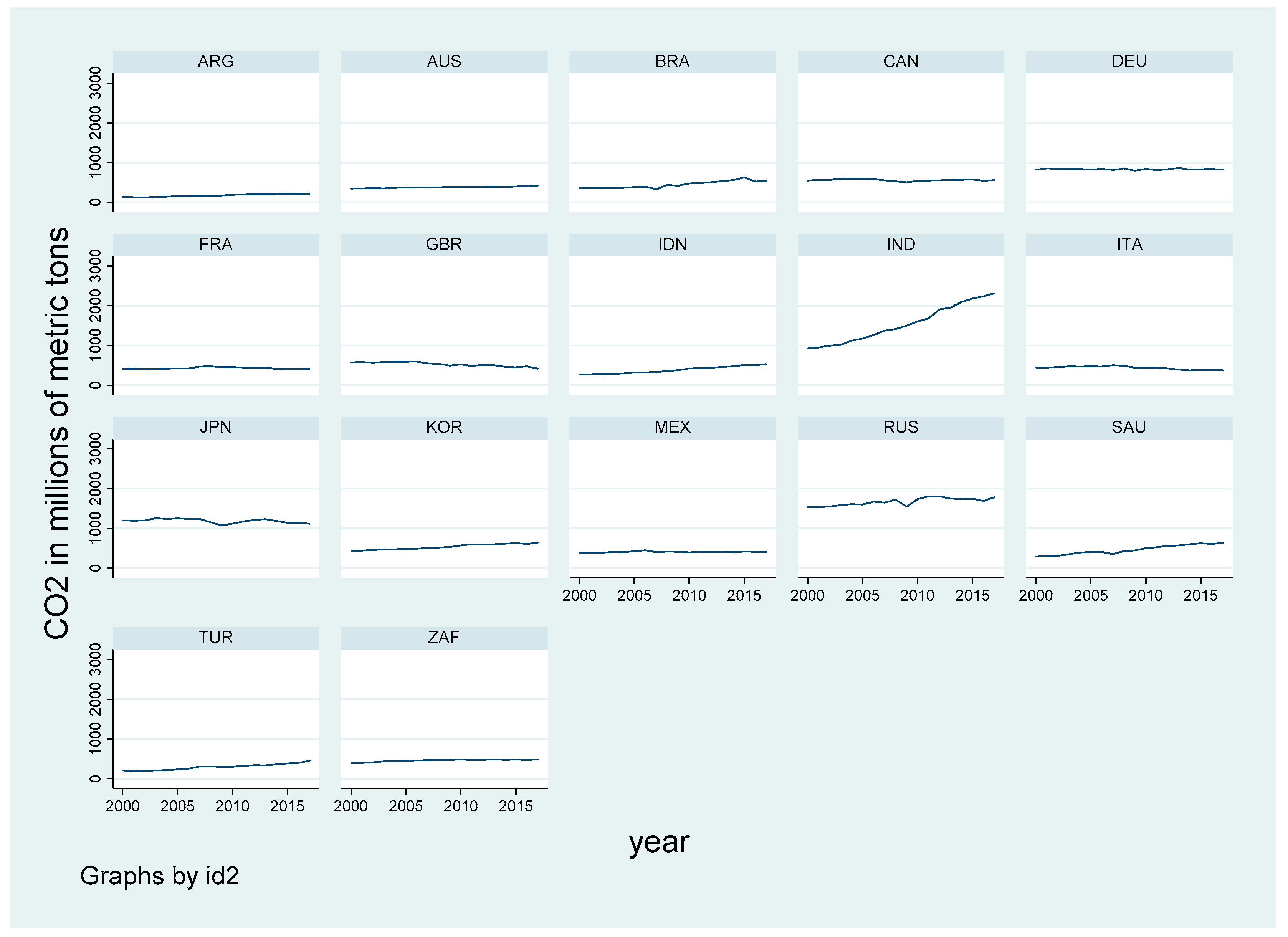
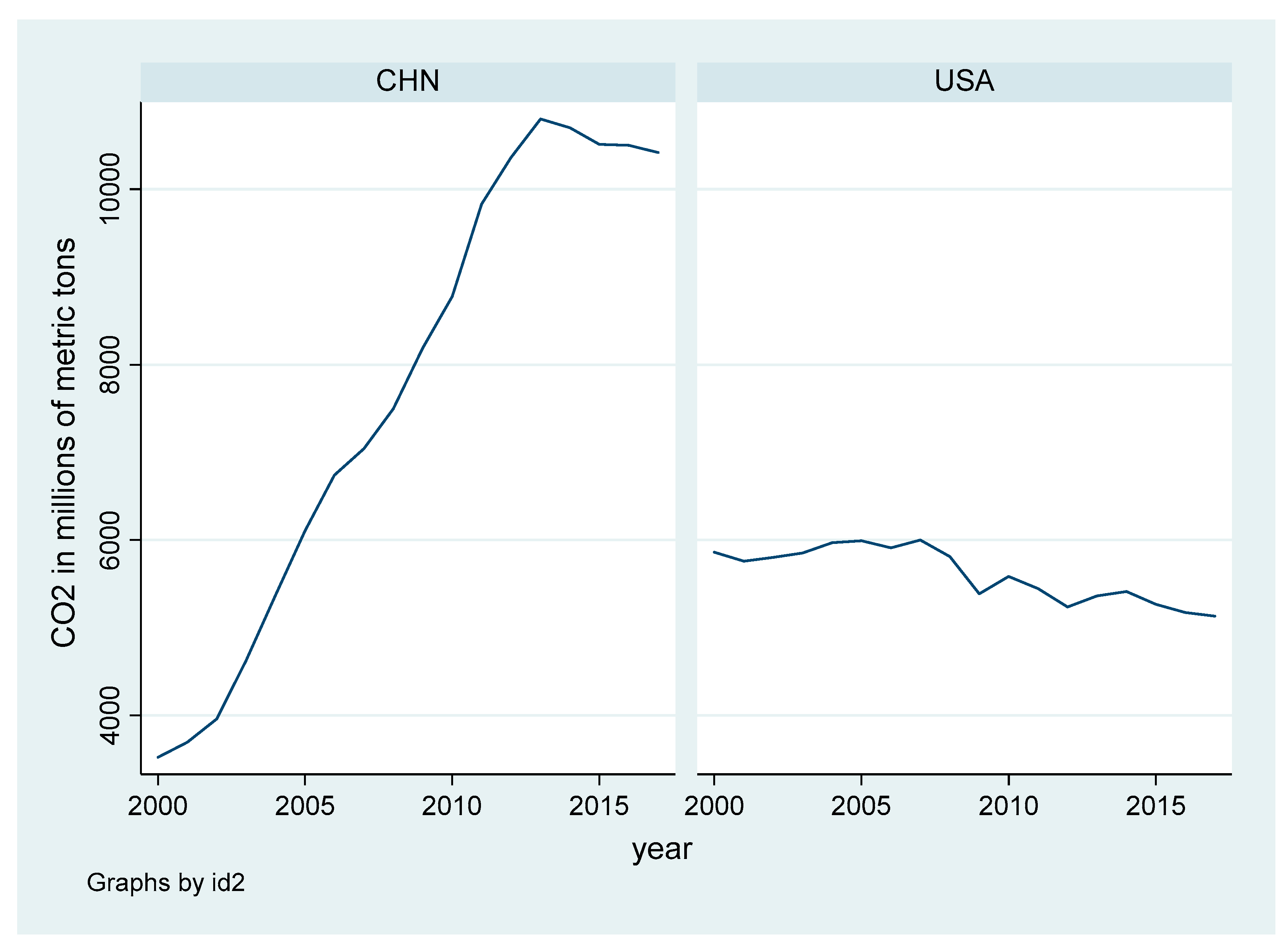
CO₂ emissions for most of the countries show a relatively flat pattern between 2000 and 2017 (Figure 1). Some countries like India experienced a large increase in emissions over the time period. China experienced a huge increase in emissions up to 2013 (10,800 million tonnes of CO₂), after which emissions declined due in part to changes in economic structure (Figure 2) [53]. US carbon emissions peaked at just about 6000 million tonnes of CO₂ in 2007 and have been experiencing a steady decrease in emissions since then due to fuel switching in power generation (coal to natural gas and renewables) and a decrease in industrial fuel use (Figure 2).

Summary statistics for CO₂, CO₂/E, E/GDP, GDP/POP, and POP indicate that CO₂ emissions are, on average, higher after the financial crisis (

Table 2. Summary statistics.

Variable	Obs	Mean	Std. D.	Min	Max
2001–2007
CO2	133	1113.96	1624.40	120.85	7043.43
CO2/E	133	59.32	12.62	31.18	86.91
E/GDP	133	6.00	2.39	2.96	11.91
GDP/POP	133	25,479.33	14,816.12	2830.72	51,005.43
POP	133	213.73	355.00	19.27	1336.80
2011–2017
CO2	133	1445.39	2412.82	192.53	10,801.77
CO2/E	133	59.02	12.36	36.89	84.58
E/GDP	133	5.33	2.07	2.43	9.75
GDP/POP	133	29,293.95	14,975.60	4721.00	54,586.25
POP	133	233.84	389.52	22.48	1409.52

CO₂ (MMtons), CO₂/E (MMtons/Quad Btus), E/GDP (Quad Btus/millions of real US dollars), GDP/POP (real US dollars per person), and POP (millions).

). In addition, GDP per capita and population are, on average, greater after the financial crisis. On average, there has been a slight reduction in carbon intensity and energy intensity between the pre-financial crisis and post-financial crisis period. In the case of CO₂ emissions, it seems that the reductions in carbon intensity and energy intensity have not been enough to compensate for the increase in CO₂ emissions coming from increased population and GDP per capita.

3. Results

3.1. The LMDI Analysis

This section presents results from the LMDI analysis. For each country, two decompositions are performed. The first decomposition covers the pre-financial crisis years 2000–2007 and the second decomposition covers the post-financial crisis years 2010–2017. Results from the additive decomposition show that for the G19, as a group, the change in CO₂ emissions post-financial crisis was less than the change in CO₂ emissions pre-financial crisis (

Table 3. Logarithmic mean Divisia index (LMDI) additive decomposition.

Country	Year	ΔCO2	ΔCI	ΔEI	ΔEA	ΔPOP
ARG	2007	20.555	−9.633	−8.465	27.367	11.285
ARG	2017	21.859	6.102	−0.780	2.345	14.191
AUS	2007	27.411	−23.068	−35.562	52.349	33.693
AUS	2017	32.380	−30.763	−12.448	35.540	40.051
BRA	2007	−32.431	−89.955	−21.843	50.296	29.070
BRA	2017	56.248	21.231	20.588	−16.426	30.856
CAN	2007	4.151	−41.283	−49.441	55.629	39.247
CAN	2017	19.017	−27.454	−38.536	46.911	38.096
CHN	2007	3520.278	−171.830	311.534	3172.617	207.957
CHN	2017	1639.622	−635.571	−1355.183	3286.201	344.174
DEU	2007	−7.388	−4.042	−82.423	80.515	−1.438
DEU	2017	−18.102	−15.020	−109.361	93.860	12.419
FRA	2007	60.627	47.087	−44.303	39.996	17.847
FRA	2017	−38.847	−7.760	−67.768	22.981	13.701
GBR	2007	−25.482	0.309	−132.440	83.673	22.976
GBR	2017	−107.478	−53.780	−118.347	43.875	20.774
IDN	2007	62.281	−0.423	−40.340	74.283	28.761
IDN	2017	108.252	42.864	−109.070	134.196	40.262
IND	2007	446.135	−0.126	−92.192	409.870	128.584
IND	2017	705.716	47.320	−212.426	707.566	163.256
ITA	2007	57.452	32.781	−13.855	22.089	16.437
ITA	2017	−70.610	−18.985	−50.412	1.333	−2.546
JPN	2007	38.979	19.568	−89.348	99.509	9.250
JPN	2017	−4.739	110.281	−201.449	95.763	−9.333
KOR	2007	81.054	−25.916	−49.525	140.249	16.246
KOR	2017	66.865	−13.178	−44.664	107.559	17.148
MEX	2007	17.011	−41.176	3.802	16.967	37.419
MEX	2017	9.045	−9.074	−60.022	39.499	38.643
RUS	2007	108.870	−29.116	−591.156	764.855	−35.714
RUS	2017	46.483	−70.183	−42.256	148.682	10.241
SAU	2007	62.393	−46.467	31.061	14.986	62.812
SAU	2017	129.230	4.090	−21.388	43.277	103.251
TUR	2007	100.328	20.316	−8.569	64.443	24.138
TUR	2017	150.012	18.798	−33.223	123.866	40.571
USA	2007	139.197	8.965	−901.593	652.706	379.118
USA	2017	−452.159	−462.628	−771.519	514.276	267.713
ZAF	2007	66.187	−12.131	−47.797	88.873	37.241
ZAF	2017	−4.649	−5.876	−60.344	16.130	45.441
G19	2007	4747.608	−366.140	−1862.455	5911.272	1064.929
G19	2017	2288.145	−1099.586	−3288.608	5447.434	1228.909
Developed	2007	294.947	40.317	−1348.965	1086.466	517.130
Developed	2017	−640.538	−506.109	−1369.840	854.539	380.875
Emerging	2007	4452.661	−406.457	−513.490	4824.806	547.799
Emerging	2017	2928.683	−593.477	−1918.768	4592.895	848.034

CO₂ is measured in millions of metric tons (MMtons).

). The biggest change was for the developed countries (Australia, Canada, France, Germany, Great Britain, Italy, Japan, and the US), where the change in CO₂ emissions in the post-financial crisis period was negative. For both developed countries and emerging countries, carbon intensity and energy intensity showed decreases in the post-financial crisis period. For emerging countries, the population effect was greater in the post-financial crisis period.

Country groupings can, however, mask individual country trends. For Argentina, Australia, Brazil, Canada, India, Indonesia, Saudi Arabia, and Turkey, the change in CO₂ emissions post-financial crisis was greater than the change in CO₂ emissions pre-financial crisis (Table 3). In other words, these countries experienced increases in CO₂ emissions over the period 2010–2017 that were greater than over the period 2000–2007. For example, in the case of Argentina, carbon emissions increased by 20.6 MMtons over the pre-financial crisis period and 21.9 MMtons over the post-financial crisis period. Notice that two of these countries are developed countries and major commodity exporters. Australia and Canada are similar in many ways, since both are small open economies and major commodity exporters (coal in the case of Australia and oil in the case of Canada). Australia has not experienced a recession since 1991 and was relatively unaffected by the financial crisis due to government stimulus spending and commodity (coal) exports. Canada was affected by the financial crisis, although not to the extent that the US was. After the financial crisis, operations in the oil sands ramped up production, which is a major source of carbon dioxide emissions. The oil sands account for approximately 9% of Canada’s GHG emissions [54].

Even though China recorded an increase in CO₂ emissions over the post-financial crisis that was less than over the pre-financial crisis, the post-financial crisis value of 1640 MMtons was the largest increase in CO₂ emissions post-financial crisis for any country studied. The next greatest increase in carbon dioxide emissions post-financial crisis was 706 MMtons (India).

Germany and Great Britain experienced decreases in CO₂ emission over both subsamples, which indicates strong continued support for reducing carbon dioxide emissions. In the case of Germany, CO₂ emissions decreased by 7.4 MMtons during the pre-financial crisis period and decreased by 18.4 MMtons in the post-financial crisis period. For Great Britain, CO₂ emissions decreased by 25.5 MMtons during the pre-financial crisis period and decreased by 107.5 MMtons in the post-financial crisis period. The largest factor for decreasing carbon emissions in Great Britain is a cleaner fuel mix in electricity generation, as coal was switched for natural gas and renewables [55]. Reduced fuel consumption by business and industry also contributed to the reduction in carbon dioxide emissions.

Among the BRICS countries, China, Russia, and South Africa recorded an increase in CO₂ emissions post-financial crisis that was smaller than over the pre-financial crisis period. Brazil and India recorded increases. Brazil experienced a decrease in emissions over the pre-financial period and then recorded a large increase in emissions over the post-financial crisis period. The post-financial crisis period encompassed the 2014 recession, which included the impeachment of the former president, political dissatisfaction, and a softening of commodity exports. Agriculture and activities associated with illegal deforestation contributed to the increase in post-financial crisis carbon dioxide emissions. In addition, the Brazilian government reduced environmental regulations in exchange for political support [56].

As an example of how to interpret the results in Table 3, consider the year 2007 for Argentina. Between 2000 and 2007, CO₂ emissions increased by 20.555 MMtons. The change in economic activity and population resulted in increases of 27.367 and 11.285 MMtons, respectively. Improvements in carbon intensity and energy intensity reduced carbon dioxide emissions by 9.663 and 8.465 MMtons, respectively. If there had been no change in energy intensity over this time period, carbon dioxide emission would have been 29.019 MMtons.

The carbon intensity effect is smaller in the post-financial crisis period for Australia, China, Germany, France, Great Britain, Italy, Russia, Turkey, and the USA (Table 3). The energy intensity effect is smaller in the post-financial crisis period for China, German, France, India, Indonesia, Italy, Japan, Mexico, Saudi Arabia, Turkey, and South Africa. China is the only BRICS country to record changes in CO₂ emissions, carbon intensity and energy intensity in the post-financial crisis period that were lower than their respective values in the pre-financial crisis period. Compared to the pre-financial crisis period, Germany, France, and Italy also recorded lower CO₂ emissions, carbon intensity and energy intensity in the post-financial crisis period. In the case of Italy, however, the population effect was negative, and the economic activity effect was positive but very small. The economic activity effect is smaller in the post-financial crisis period for Argentina, Australia, Brazil, Canada, France, Great Britain, Italy, Japan, South Korea, Russia, the United States, and South Africa. Most of these countries are developed countries. Brazil is the only country to record a negative economic effect in the post-financial crisis period, and this was due to the 2014 recession. The population effect is smaller in the post-financial crisis period for Canada, France, Great Britain, Italy, Japan, and the USA. These countries are all developed nations. In the post-financial crisis period, only Italy and Japan recorded negative values for the population effect. For most countries, reductions in energy intensity had a larger impact on reducing carbon dioxide emissions than reductions in carbon intensity, which is consistent with much of the published literature.

The Kaya identity is related to the IPAT model (I = CO₂ emissions, P = population, A = affluence (GDP per capita), T = technology (energy intensity)). As a robustness check a fixed effects regression was used to estimate an IPAT model in natural logarithm form for the pre-financial crisis and post-financial crisis periods. For each variable, in each period, the estimated coefficient is positive, close to unity, and statistically significant. This confirms the importance of population, affluence, and energy intensity in explaining CO₂ emissions.

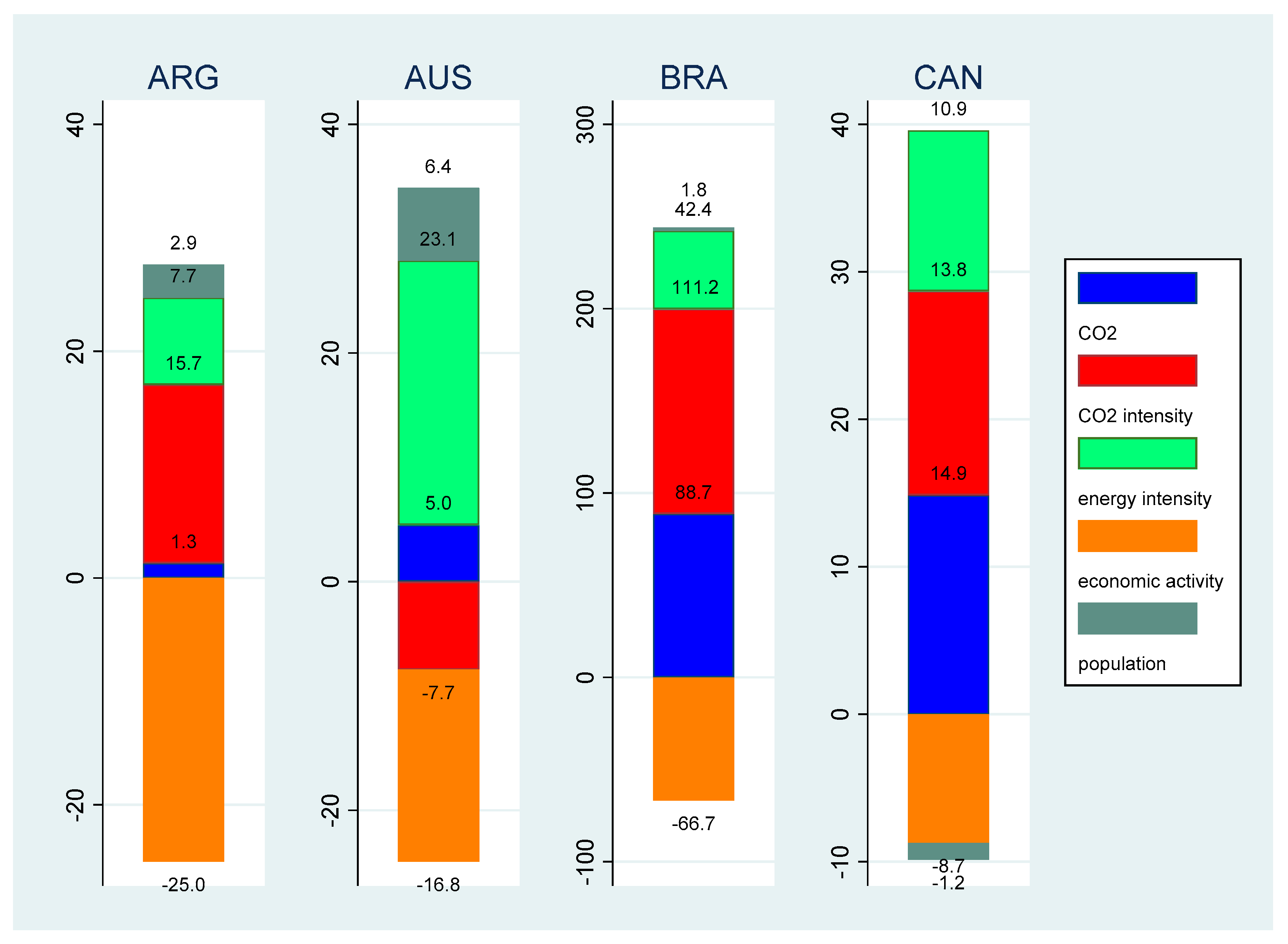
Figure 3 presents a graphical comparison of the difference in post-financial crisis and pre-financial crisis results from Table 3 for Argentina, Australia, Brazil and Canada. For each country, the 2007 values for each decomposition factor are subtracted from their respective 2017 values to determine which factor exhibited the greatest change between the two subperiods. For Argentina, the biggest factor was the decrease in economic activity. For Australia, the biggest factor was an increase in energy intensity. For Brazil and Canada, the biggest factor was an increase in carbon intensity.

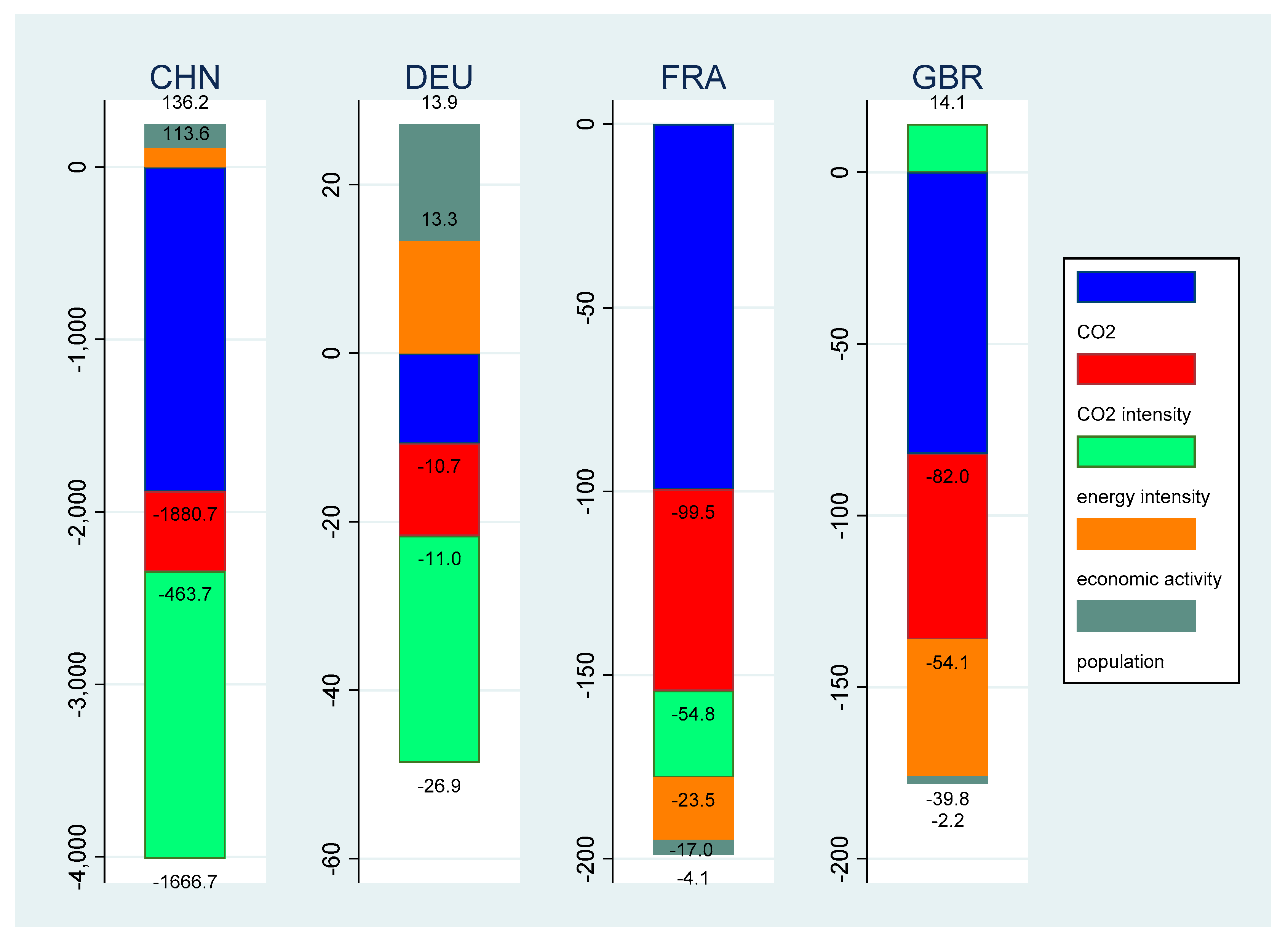
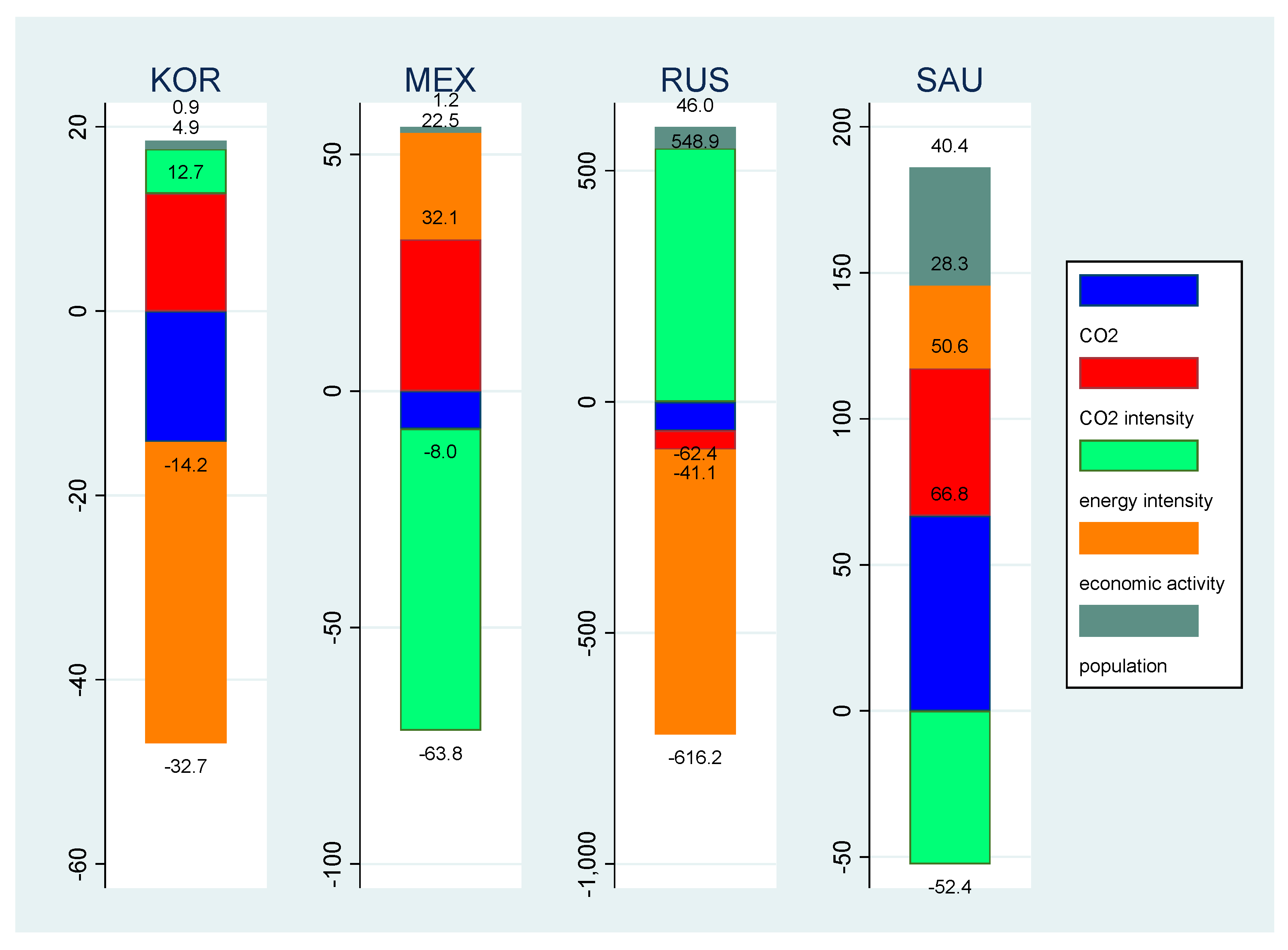
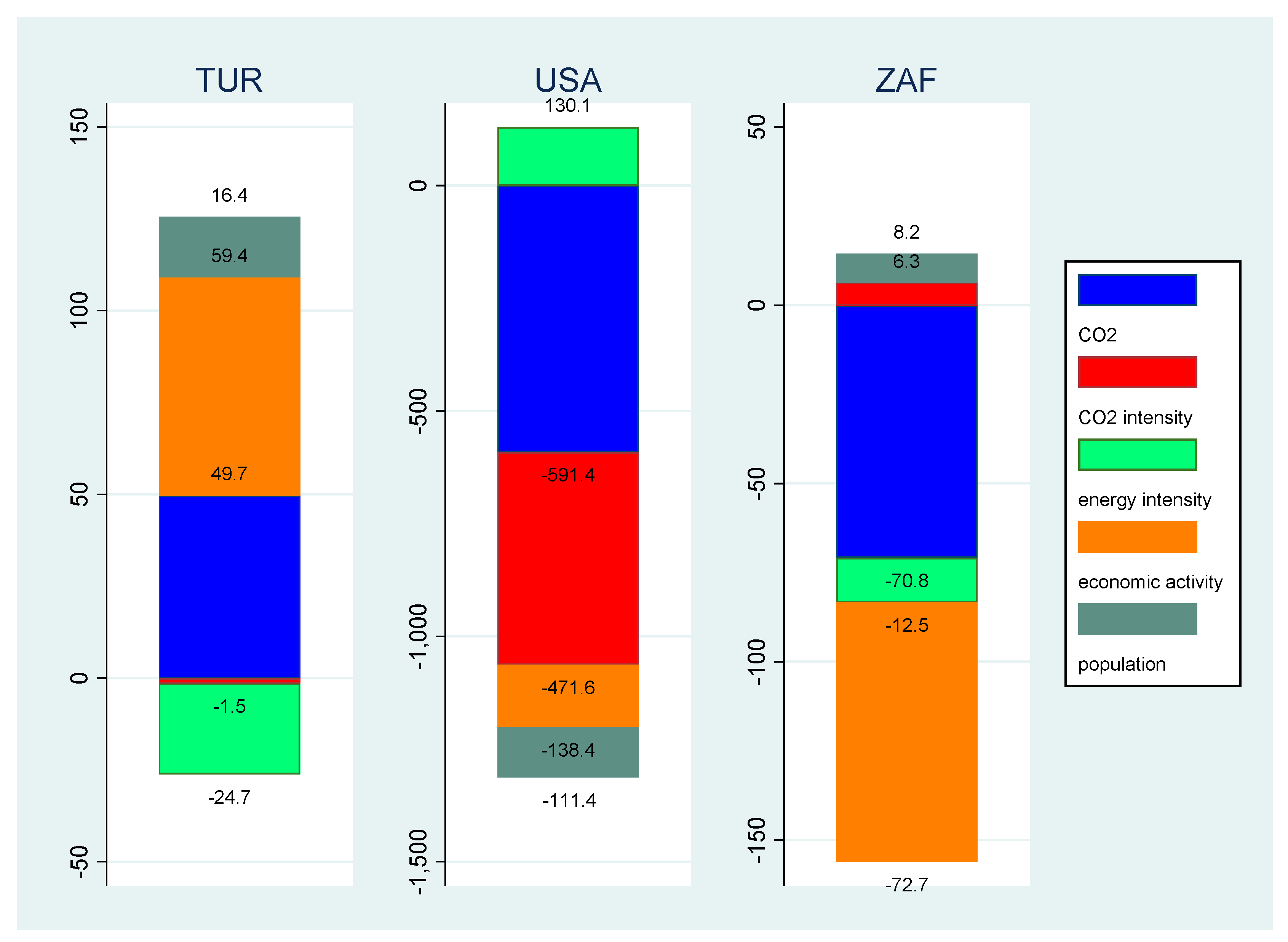
For China and Germany, the biggest factor was a decrease in energy intensity. For France and Great Britain, the biggest factor was a decrease in carbon intensity (Figure 4). For Indonesia, the biggest factor was a decrease in energy intensity (Figure 5). For India, the biggest factor was an increase in economic activity. For Italy, the biggest factor was a decrease in carbon intensity. For Japan, the biggest factor was a decrease in energy intensity. For South Korea, the biggest factor was a decrease in economic activity (Figure 6). For Mexico, the biggest factor was a decrease in energy intensity. For Russia, the biggest factor was an increase in energy intensity and for Saudi Arabia the biggest factor was a decrease in energy intensity. For Turkey, the biggest factor was an increase in economic activity (Figure 7). For the USA, the biggest factor was a decrease in carbon intensity. For South Africa, the biggest factor was a decrease in economic activity. In summary, when looking at the change in decomposition factors between the post-financial crisis and pre-financial crisis periods, carbon intensity was the most important factor affecting changes in carbon dioxide emissions for six countries, energy intensity was the most important factor for seven countries and economic activity was the most important factor for six countries.

LMDI multiplicative decomposition is another way of looking at the decomposition of CO₂ emissions (

Table 4. LMDI multiplicative decomposition.

Country	Year	DCO2	DCI	DEI	DEA	DPOP
ARG	2007	1.148	0.937	0.945	1.201	1.079
ARG	2017	1.116	1.031	0.996	1.012	1.074
AUS	2007	1.080	0.938	0.905	1.157	1.099
AUS	2017	1.084	0.926	0.969	1.093	1.105
BRA	2007	0.909	0.766	0.937	1.160	1.090
BRA	2017	1.119	1.043	1.042	0.968	1.063
CAN	2007	1.008	0.927	0.914	1.107	1.074
CAN	2017	1.035	0.951	0.932	1.089	1.072
CHN	2007	1.999	0.967	1.063	1.867	1.042
CHN	2017	1.187	0.936	0.868	1.409	1.037
DEU	2007	0.991	0.995	0.904	1.104	0.998
DEU	2017	0.978	0.982	0.877	1.120	1.015
FRA	2007	1.148	1.113	0.904	1.095	1.041
FRA	2017	0.915	0.982	0.856	1.054	1.032
GBR	2007	0.956	1.001	0.790	1.161	1.042
GBR	2017	0.795	0.891	0.776	1.098	1.045
IDN	2007	1.233	0.999	0.873	1.283	1.101
IDN	2017	1.256	1.095	0.795	1.327	1.089
IND	2007	1.483	1.000	0.922	1.436	1.120
IND	2017	1.439	1.025	0.896	1.441	1.088
ITA	2007	1.129	1.072	0.971	1.048	1.035
ITA	2017	0.842	0.955	0.884	1.003	0.994
JPN	2007	1.032	1.016	0.929	1.085	1.008
JPN	2017	0.996	1.104	0.835	1.089	0.992
KOR	2007	1.189	0.946	0.899	1.350	1.035
KOR	2017	1.117	0.978	0.929	1.195	1.029
MEX	2007	1.044	0.901	1.010	1.044	1.099
MEX	2017	1.023	0.978	0.861	1.103	1.101
RUS	2007	1.071	0.982	0.690	1.616	0.978
RUS	2017	1.027	0.961	0.976	1.088	1.006
SAU	2007	1.215	0.865	1.102	1.048	1.216
SAU	2017	1.258	1.007	0.963	1.080	1.201
TUR	2007	1.489	1.084	0.967	1.291	1.101
TUR	2017	1.502	1.052	0.914	1.400	1.116
USA	2007	1.024	1.002	0.859	1.116	1.066
USA	2017	0.919	0.917	0.866	1.101	1.051
ZAF	2007	1.167	0.972	0.894	1.231	1.091
ZAF	2017	0.990	0.988	0.882	1.034	1.099

). Values greater than unity indicate positive increases over the time period under consideration, while values less than unity indicated reductions over the time period. Multiplicative decomposition gives information on the direction of the changes in decomposition as well as the rates of change over specified time periods. In the case of Argentina, for example, CO₂ emissions increased between 2000 and 2007 by a factor of 1.148 and between 2010 and 2017 by a factor of 1.116. In the post-financial period, the carbon intensity component increased by a factor of 1.031, the energy intensity component increased by a factor of 0.996, the economic activity component increased by a factor of 1.012, and the population component increased by a factor of 1.074.

The largest rates of change in CO₂ in the post-recession period were observed in Turkey (1.502), India (1.439), and Saudi Arabia (1.258). The smallest rates of change in CO₂ in the post-recession period were observed in Great Britain (0.795), Italy (0.842), and France (0.915). Great Britain, USA, and Australia had the smallest rates of change in the carbon intensity factor, while Japan, Indonesia, and Turkey had the largest increase. The smallest rates of change in the energy intensity factor occurred in Great Britain, Indonesia, and Japan. The largest rates of change in the energy intensity factor occurred in Brazil, Argentina, and Russia. The smallest rates of change in the economic activity factor occurred in Brazil, Italy, and Argentina, while the largest rates of change occurred in India, China, and Turkey. Japan, Italy, and Russia had the lowest rates of change in the population effect, while Saudi Arabia, Turkey, and Australia had the largest rates of change. In general, the economic activity factor and population factor are most important for large fast-growing developing countries.

For most countries, the largest contributor to CO₂ emission rates of change in the post-recession period was economic activity (13 countries) or population (5). Japan is the outlier, because the largest contrition to CO₂ emission rates of change comes from carbon intensity. This is due to how the 2011 Fukushima nuclear disaster altered the energy supply in Japan [57,58,59]. The Japanese nuclear power sector was shut down in 2012, but some reactors have been allowed to come back online since then. For 16 countries, the smallest contributor to CO₂ emission rates of change was energy intensity.

3.2. Decoupling Analysis

The result from Tapio decoupling between CO₂ and GDP are reported in

Table 5. Tapio decoupling.

Country	Year	ΔCO2/CO2	ΔGDP/GDP	e	Decoupling
ARG	2007	0.1478	0.2958	0.4995	Weak decoupling
ARG	2017	0.1161	0.0866	1.3399	Expansive negative decoupling
AUS	2007	0.0795	0.2716	0.2929	Weak decoupling
AUS	2017	0.0844	0.2081	0.4053	Weak decoupling
BRA	2007	−0.0915	0.2646	−0.3457	Strong decoupling
BRA	2017	0.1187	0.0292	4.0660	Expansive negative decoupling
CAN	2007	0.0076	0.1892	0.0402	Weak decoupling
CAN	2017	0.0353	0.1675	0.2105	Weak decoupling
CHN	2007	0.9992	0.9450	1.0574	Expansive coupling
CHN	2017	0.1868	0.4610	0.4051	Weak decoupling
DEU	2007	−0.0090	0.1016	−0.0886	Strong decoupling
DEU	2017	−0.0216	0.1366	−0.1579	Strong decoupling
FRA	2007	0.1480	0.1408	1.0515	Expansive coupling
FRA	2017	−0.0853	0.0878	−0.9711	Strong decoupling
GBR	2007	−0.0444	0.2093	−0.2121	Strong decoupling
GBR	2017	−0.2053	0.1482	−1.3851	Strong decoupling
IDN	2007	0.2326	0.4134	0.5626	Weak decoupling
IDN	2017	0.2561	0.4441	0.5767	Weak decoupling
IND	2007	0.4829	0.6088	0.7931	Weak decoupling
IND	2017	0.4393	0.5673	0.7744	Weak decoupling
ITA	2007	0.1287	0.0846	1.5218	Expansive negative decoupling
ITA	2017	−0.1583	−0.0030	53.5593	Recessive decoupling
JPN	2007	0.0325	0.0933	0.3482	Weak decoupling
JPN	2017	−0.0042	0.0803	−0.0526	Strong decoupling
KOR	2007	0.1894	0.3977	0.4761	Weak decoupling
KOR	2017	0.1173	0.2297	0.5104	Weak decoupling
MEX	2007	0.0440	0.1478	0.2981	Weak decoupling
MEX	2017	0.0228	0.2147	0.1061	Weak decoupling
RUS	2007	0.0707	0.5806	0.1218	Weak decoupling
RUS	2017	0.0268	0.0946	0.2832	Weak decoupling
SAU	2007	0.2146	0.2743	0.7823	Weak decoupling
SAU	2017	0.2576	0.2968	0.8680	Expansive coupling
TUR	2007	0.4890	0.4212	1.1610	Expansive coupling
TUR	2017	0.5024	0.5624	0.8934	Expansive coupling
USA	2007	0.0237	0.1900	0.1250	Weak decoupling
USA	2017	−0.0810	0.1572	−0.5150	Strong decoupling
ZAF	2007	0.1673	0.3428	0.4880	Weak decoupling
ZAF	2017	−0.0097	0.1371	−0.0704	Strong decoupling

. Consistent with the decomposition analysis, the changes are calculated over seven-year intervals (2000–2007, 2010–2017). Twenty entries are weak decoupling, nine are strong decoupling, five are expansive coupling, three are expansive negative decoupling, and one is recessive decoupling. Weak decoupling is by far the most popular state. Nine countries experienced a change in decoupling state between the pre-financial crisis period and the post-financial crisis period (Argentina, Brazil, China, France, Italy, Japan, Saudi Arabia, USA, and South Africa). Germany, France, Great Britain, Japan, the United States and South Africa experienced strong decoupling in the post-financial crisis period. Two countries that have experienced surprising shifts towards less decoupling are Brazil (strong decoupling pre-financial crisis to expansive negative decoupling post-financial crisis) and Italy (expansive negative decoupling pre-financial crisis to recessive decoupling post-financial crisis). Brazil’s 2014 recession affected economic activity and policy related to energy and the environment. Italy has, in some ways, entered a “perma-recession”. Massive government debt, a historic debt to GDP ratio, fear of systemic risk, and a cloudy political situation limits the ability of the government to focus on energy policy. Under European Union rules, Italy’s debt problems and financial situation prevent government deficit spending to help grow the economy [60]. Notice that in the case of Italy, the 2017 CO₂ elasticity is negative and the GDP elasticity is negative, which is consistent with a slowdown in carbon dioxide emissions associated with a slowdown in economic activity. The green stimulus packages implemented by some countries may be one positive benefit stemming from the financial crisis [8] and may help to explain why some countries transitioned from weak decoupling to strong decoupling.

4. Discussion

In general, reductions in carbon intensity and energy intensity reduce CO₂ emissions, while increases in economic activity and population increase CO₂ emissions. This is consistent with the existing literature [10,24,25]. For most countries, reductions in energy intensity have had a bigger impact on reducing CO₂ emissions than reductions in carbon intensity, and this is true in both the pre-financial crisis period and post-financial crisis period. For most countries studied, increases in economic activity are the largest contributor to increasing CO₂ emissions, which is consistent with the existing literature [10,24]. Saudi Arabia is an exception, because the population effect was the greatest contributor to CO₂ emissions in both the pre-financial crisis and post-financial crisis periods. For each country, the energy intensity effect is negative in the post-financial crisis period except for Brazil. The 2014 recession in Brazil led to a negative economic effect and a positive energy intensity effect, with the population effect being the largest contributor to CO₂ emissions.

China is the only BRICS country to record changes in CO₂ emissions, carbon intensity and energy intensity in the post-financial crisis period that were lower than their respective values in the pre-financial crisis period. Fuel switching from fossil fuels to renewables, capital equipment modernization, industry sector realignment, and energy related technological improvements are important contributions to reducing carbon dioxide emissions in China [61]. Compared to the pre-financial crisis period, Germany, France, and Italy also recorded lower CO₂ emissions, carbon intensity and energy intensity in the post-financial crisis period, although these reductions were matched with a negative population effect and a negligible economic activity effect in the case of Italy. Continued improvements in reducing CO₂ emissions, carbon intensity and energy intensity are hard to come by, as only four out of nineteen countries were able to achieve this. These results are important, because reductions in carbon intensity and energy intensity are major factors in a country’s transition to a low-carbon economy.

The decoupling analysis reveals some important results. Germany, France, Great Britain, Japan, the United States and South Africa experienced strong decoupling in the post-financial crisis period. Strong decoupling is important for environmental sustainability, because this means that carbon dioxide emissions are declining while the economy is growing. Most of the other countries are characterized as weak decoupling.

Germany and France are the two countries that stand out as leaders among the G19. In the post-financial crisis period, they have shown reductions in carbon emissions, carbon intensity and energy intensity and both are characterized as strong decoupling. These results are consistent with the findings from some recent policy studies. While designing an energy policy is one thing, maintaining the intended direction of the policy can be challenging across time. In the case of Germany, cross-partisan policy consistency, shared goals between political leaders and renewable energy advocates, a strong social movement for renewable energy, and decentralized energy policies have been major factors to Germany’s continued success on transitioning to a low-carbon economy [20]. Nuclear power is the primary energy source in France’s transition to a low-carbon economy [62]. France’s almost sole focus on electricity development means that other sectors like transportation have been neglected. In France, oil remains an important fuel for transportation under most future energy consumption scenarios, but this may change if there is widespread adoption of electric vehicles. The results of this present paper are also consistent with those of Midova et al. [63], who study low-carbon scenarios of six north-west European countries (Netherlands, Germany, France, Denmark, the UK, and Belgium). In ranking these countries on ten criteria regarding low-carbon energy scenario design, Germany comes out on top, followed by the UK. France’s heavy reliance on nuclear power makes it less receptive to technological innovation for other renewable energy sources. Results from this present study show that Great Britain, the United States, and South Africa have also shown strong performance in reducing carbon dioxide emissions and energy intensity in the post-financial crisis period.

Among the developed countries, Australia and Canada are laggards. These countries are small open-economy natural resource-intensive exporters that have increased CO₂ emissions post-financial crisis. For Australia, the biggest change between the pre-financial period and post-financial period was an increase in energy intensity. For Canada, the biggest change was an increase in carbon intensity. For these countries, a reliance on the natural resource extraction (coal and oil) sector make it difficult to decrease carbon dioxide emissions. Den Elzen et al. [56] find that by comparing projected GHGs with 2030 target emissions, both Australia and Canada are unlikely to meet their nationally determined contributions (NDCs). Further increases in reducing carbon intensity and energy intensity can be obtained by decarbonizing energy supply and increasing energy efficiency in transportation, buildings, and industry. Decarbonizing energy supply is, however, at odds with maintaining fossil fuel exports.

Argentina, Brazil, India, Indonesia, Saudi Arabia, and Turkey are developing countries that experienced increases in CO₂ emissions over the period 2010–2017 that were greater than that over the period 2000–2007. Argentina and Brazil are the two countries experiencing CO₂ emission growth in the post-financial crisis period greater than GDP growth. Both of these countries have unusual economic situations (a deep recession in Brazil and a debt crisis in Argentina), which creates problems for developing and implementing clean energy policy. For these countries, a return to more orderly economic conditions must first precede a commitment to energy policy focusing on reducing carbon intensity and energy intensity. Of the BRICS countries, China, Russia, and South Africa recorded lower increases in CO₂ emissions post-financial crisis. China’s reductions in carbon intensity and energy intensity post-financial crisis are impressive but China’s carbon dioxide emission increases over this period are the largest of the countries studied and due to the large increases in economic activity and population. Nevertheless, Den Elzen et al. [56] find that China is on track to meet its NDC targets for GHG emissions. China, through a series of five-year plans, has ambitious targets to lower carbon intensity and energy intensity [64]. India, like China, suffers high vulnerability from climate change, but India has no strong numeric targets for their energy policy unlike China [64]. Sarangi et al. [65] find that the Indian government’s feed-in tariff policy has been successful in improving electricity accessibility and diversifying the electricity supply.

5. Conclusions and Policy Implications

The focus of this research is to study how energy related CO₂ emissions and their driving factors after the financial crisis compare to the period before the financial crisis. The logarithmic mean Divisia index (LMDI) method is used to decompose changes in country level CO₂ emissions into contributing factors representing carbon intensity, energy intensity, economic activity, and population. The analysis is conducted for a group of 19 major countries which form the core of the G20. The LMDI decomposition analysis reveals some important results. For the G19, as a group, the increase in CO₂ emissions post-financial crisis was less than the increase in CO₂ emissions pre-financial crisis. A decrease in energy intensity was the biggest driver behind reducing CO₂ emissions, while an increase in economic activity was the biggest factor increasing CO₂ emissions. There are, however, differences between countries. Germany and Great Britain are the only two countries to record negative changes in CO₂ emissions over both periods. Germany and France are the two countries that stand out as leaders among the G19 because, compared to the pre-financial crisis period, they recorded lower CO₂ emissions, carbon intensity and energy intensity in the post-financial crisis period and both are characterized as strong decoupling. Together, these two countries accounted for a reduction of 56.95 million metric tons in CO₂ emissions in the post-financial crisis period. This value was very similar to Brazil’s increase in emissions (56.25 MMtons) during the same period. Argentina, Australia, Brazil, Canada, India, Indonesia, Saudi Arabia, and Turkey, however, experienced increases in CO₂ emissions over the period 2010–2017 that were greater than over the period 2000–2007. For Argentina, Brazil, Canada, and Saudi Arabia, the biggest factor behind this increase was an increase in carbon emission intensity. For Australia, the biggest factor was an increase in energy intensity. For India, Indonesia and Turkey, the biggest factor was an increase in economic activity. Reducing CO₂ emissions in Australia, Canada, and Saudi Arabia is challenging because these countries are major exporters of fossil fuels. For these countries, a successful sustainable energy policy requires a decoupling of the fossil fuel export sector from the rest of the economy. An energy policy recommendation for Argentina, Brazil, India, Indonesia and Turkey is to set and maintain stronger NDC goals.

While the main focus of this paper is to compare carbon dioxide emissions post-financial crisis with those pre-financial crises for the G19 countries it is now apparent that a new crisis is unfolding. This time, however, the crisis is a health crisis. It is difficult to compare the 2008–2009 financial crisis with the current COVID-19 pandemic because the pandemic is a health crisis with far greater impacts than what was experienced during the financial crisis. Since COVID-19 has wider ranging impacts than the financial crisis, the impact on reducing CO₂ emissions will be greater and could affect weather patterns.

In summary, 11 of the 19 countries studied showed increases in carbon dioxide emissions over the post-financial crisis period that were lower than over the pre-financial crisis period. This is a step in the right direction for meeting NDCs and global climate change policies but, given the importance of the G19 to the world economy, all G19 countries must act as leaders in the fight against climate change and reduce their emissions. There are several policy implications. The goal should be for all G19 countries to exhibit strong decoupling but only six countries showed strong decoupling in the post-financial crisis period. The chair of the G20 rotates on a yearly basis, which means the G20 agenda for each year depends upon the interests of the chair. An important policy recommendation is for a non-partisan G20 energy policy focused on continuous improvements in reducing carbon intensity and energy intensity through fuel switching and changes in industry structure because this is crucial for future reductions in carbon dioxide emissions. A further policy recommendation is for the G20 environmental ministers to be allowed greater involvement in decision making [66]. The G20 can be a leader in meeting the Paris Climate Change Agreement but all countries must be fully committed to reducing carbon dioxide emissions and cooperate towards this shared goal.

References

- Demyanyk, Y.; Van Hemert, O. Understanding the Subprime Mortgage Crisis. Rev Financ. Stud. 2011, 24, 1848–1880. [Google Scholar] [CrossRef]
- Lewis, M. The Big Short: Inside the Doomsday Machine, reprint ed.; WW Norton: New York, NY, USA, 2011; ISBN 978-0-393-33882-9. [Google Scholar]
- Gupta, A. Chapter 1—Climate Change and Kyoto Protocol: An Overview. In Handbook of Environmental and Sustainable Finance; Ramiah, V., Gregoriou, G.N., Eds.; Academic Press: San Diego, CA, USA, 2016; pp. 3–23. ISBN 978-0-12-803615-0. [Google Scholar]
- Kanellakis, M.; Martinopoulos, G.; Zachariadis, T. European energy policy—A review. Energy Policy 2013, 62, 1020–1030. [Google Scholar] [CrossRef]
- Giedraitis, V.; Girdenas, S. Feeling the Heat: Financial Crises and Their Impact on Global Climate Change. Perspect. Innov. Econ. Bus. (PIEB) 2010, 4, 7–10. [Google Scholar] [CrossRef]
- Siddiqi, T.A. The Asian Financial Crisis—Is it good for the global environment? Glob. Environ. Chang. 2000, 10, 1–7. [Google Scholar] [CrossRef]
- Jalles, J.T. Crises and emissions: New empirical evidence from a large sample. Energy Policy 2019, 129, 880–895. [Google Scholar] [CrossRef] [Green Version]
- Mundaca, L.; Luth Richter, J. Assessing ‘green energy economy’ stimulus packages: Evidence from the U.S. programs targeting renewable energy. Renew. Sustain. Energy Rev. 2015, 42, 1174–1186. [Google Scholar] [CrossRef] [Green Version]
- Andreoni, V. The energy metabolism of countries: Energy efficiency and use in the period that followed the global financial crisis. Energy Policy 2020, 139, 111304. [Google Scholar] [CrossRef]
- Dong, K.; Hochman, G.; Timilsina, G.R. Do drivers of CO2 emission growth alter overtime and by the stage of economic development? Energy Policy 2020, 140, 111420. [Google Scholar] [CrossRef]
- Roinioti, A.; Koroneos, C. The decomposition of CO2 emissions from energy use in Greece before and during the economic crisis and their decoupling from economic growth. Renew. Sustain. Energy Rev. 2017, 76, 448–459. [Google Scholar] [CrossRef]
- Timma, L.; Zoss, T.; Blumberga, D. Life after the financial crisis. Energy intensity and energy use decomposition on sectorial level in Latvia. Appl. Energy 2016, 162, 1586–1592. [Google Scholar] [CrossRef]
- Thombs, R.P. Has the relationship between non-fossil fuel energy sources and CO2 emissions changed over time? A cross-national study, 2000–2013. Clim. Chang. 2018, 148, 481–490. [Google Scholar] [CrossRef]
- Woo, C.; Chung, Y.; Chun, D.; Seo, H.; Hong, S. The static and dynamic environmental efficiency of renewable energy: A Malmquist index analysis of OECD countries. Renew. Sustain. Energy Rev. 2015, 47, 367–376. [Google Scholar] [CrossRef]
- Mimouni, K.; Temimi, A. What drives energy efficiency? New evidence from financial crises. Energy Policy 2018, 122, 332–348. [Google Scholar] [CrossRef]
- Government of Canada. Canada’s Participation at the 2019 G20 Summit. Available online: https://www.international.gc.ca/gac-amc/campaign-campagne/g20/index.aspx?lang=eng (accessed on 8 April 2020).
- De Graaf, T.V.; Westphal, K. The G8 and G20 as Global Steering Committees for Energy: Opportunities and Constraints. Glob. Policy 2011, 2, 19–30. [Google Scholar] [CrossRef]
- Ang, B.W. The LMDI approach to decomposition analysis: A practical guide. Energy Policy 2005, 33, 867–871. [Google Scholar] [CrossRef]
- National Bureau of Economic Reserach US Business Cycle Expansions and Contractions. Available online: https://www.nber.org/cycles.html (accessed on 9 April 2020).
- Cheung, G.; Davies, P.J.; Bassen, A. In the transition of energy systems: What lessons can be learnt from the German achievement? Energy Policy 2019, 132, 633–646. [Google Scholar] [CrossRef]
- UNFCCC. The Paris Agreement|UNFCCC. Available online: https://unfccc.int/process-and-meetings/the-paris-agreement/the-paris-agreement (accessed on 8 April 2020).
- Ang, B.W. Decomposition analysis for policymaking in energy: Which is the preferred method? Energy Policy 2004, 32, 1131–1139. [Google Scholar] [CrossRef]
- Goh, T.; Ang, B.W.; Su, B.; Wang, H. Drivers of stagnating global carbon intensity of electricity and the way forward. Energy Policy 2018, 113, 149–156. [Google Scholar] [CrossRef]
- Yao, C.; Feng, K.; Hubacek, K. Driving forces of CO2 emissions in the G20 countries: An index decomposition analysis from 1971 to 2010. Ecol. Inform. 2015, 26, 93–100. [Google Scholar] [CrossRef]
- Chen, J.; Wang, P.; Cui, L.; Huang, S.; Song, M. Decomposition and decoupling analysis of CO2 emissions in OECD. Appl. Energy 2018, 231, 937–950. [Google Scholar] [CrossRef]
- Bhattacharyya, S.C.; Matsumura, W. Changes in the GHG emission intensity in EU-15: Lessons from a decomposition analysis. Energy 2010, 35, 3315–3322. [Google Scholar] [CrossRef]
- Kopidou, D.; Tsakanikas, A.; Diakoulaki, D. Common trends and drivers of CO2 emissions and employment: A decomposition analysis in the industrial sector of selected European Union countries. J. Clean. Prod. 2016, 112, 4159–4172. [Google Scholar] [CrossRef]
- Moutinho, V.; Moreira, A.C.; Silva, P.M. The driving forces of change in energy-related CO2 emissions in Eastern, Western, Northern and Southern Europe: The LMDI approach to decomposition analysis. Renew. Sustain. Energy Rev. 2015, 50, 1485–1499. [Google Scholar] [CrossRef]
- Chapman, A.; Fujii, H.; Managi, S. Key Drivers for Cooperation toward Sustainable Development and the Management of CO2 Emissions: Comparative Analysis of Six Northeast Asian Countries. Sustainability 2018, 10, 244. [Google Scholar] [CrossRef] [Green Version]
- Su, W.; Wang, Y.; Streimikiene, D.; Balezentis, T.; Zhang, C. Carbon dioxide emission decomposition along the gradient of economic development: The case of energy sustainability in the G7 and Brazil, Russia, India, China and South Africa. Sustainable Development 2019. [Google Scholar] [CrossRef]
- Wang, Q.; Jiang, R. Is carbon emission growth decoupled from economic growth in emerging countries? New insights from labor and investment effects. J. Clean. Prod. 2020, 248, 119188. [Google Scholar] [CrossRef]
- Lima, F.; Nunes, M.L.; Cunha, J.; Lucena, A.F.P. A cross-country assessment of energy-related CO2 emissions: An extended Kaya Index Decomposition Approach. Energy 2016, 115, 1361–1374. [Google Scholar] [CrossRef] [Green Version]
- Lima, F.; Nunes, M.L.; Cunha, J.; Lucena, A.F.P. Driving forces for aggregate energy consumption: A cross-country approach. Renew. Sustain. Energy Rev. 2017, 68, 1033–1050. [Google Scholar] [CrossRef] [Green Version]
- Moutinho, V.; Madaleno, M.; Inglesi-Lotz, R.; Dogan, E. Factors affecting CO2 emissions in top countries on renewable energies: A LMDI decomposition application. Renew. Sustain. Energy Rev. 2018, 90, 605–622. [Google Scholar] [CrossRef] [Green Version]
- Rüstemoğlu, H.; Andrés, A.R. Determinants of CO2 emissions in Brazil and Russia between 1992 and 2011: A decomposition analysis. Environ. Sci. Policy 2016, 58, 95–106. [Google Scholar] [CrossRef]
- Štreimikienė, D.; Balezentis, T. Kaya identity for analysis of the main drivers of GHG emissions and feasibility to implement EU “20–20–20” targets in the Baltic States. Renew. Sustain. Energy Rev. 2016, 58, 1108–1113. [Google Scholar] [CrossRef]
- Sun, Q.; Geng, Y.; Ma, F.; Wang, C.; Wang, B.; Wang, X.; Wang, W. Spatial–Temporal Evolution and Factor Decomposition for Ecological Pressure of Carbon Footprint in the One Belt and One Road. Sustainability 2018, 10, 3107. [Google Scholar] [CrossRef] [Green Version]
- Zhang, J.; Fan, Z.; Chen, Y.; Gao, J.; Liu, W. Decomposition and decoupling analysis of carbon dioxide emissions from economic growth in the context of China and the ASEAN countries. Sci. Total Environ. 2020, 714, 136649. [Google Scholar] [CrossRef] [PubMed]
- Kaya, Y. Impact of Carbon Dioxide Emission Control on GNP Growth: Interpretation of Proposed Scenarios; IPCC Energy and Industry Subgroup, Response Strategies Working Group: Paris, France, 1990. [Google Scholar]
- Kaya, Y.; Yokobori, K. (Eds.) Environment, Energy, and Economy: Strategies for Sustainable; United Nations Univ: Tokyo, Japan; New York, NY, USA, 1998; ISBN 978-92-808-0911-4. [Google Scholar]
- Raupach, M.R.; Marland, G.; Ciais, P.; Le Quéré, C.; Canadell, J.G.; Klepper, G.; Field, C.B. Global and regional drivers of accelerating CO2 emissions. Proc. Natl. Acad. Sci. USA 2007, 104, 10288. [Google Scholar] [CrossRef] [PubMed] [Green Version]
- Tapio, P. Towards a theory of decoupling: Degrees of decoupling in the EU and the case of road traffic in Finland between 1970 and 2001. Transp. Policy 2005, 12, 137–151. [Google Scholar] [CrossRef] [Green Version]
- Jorgenson, A.K.; Clark, B. Are the Economy and the Environment Decoupling? A Comparative International Study, 1960–2005. Am. J. Sociol. 2012, 118, 1–44. [Google Scholar] [CrossRef]
- Schandl, H.; Hatfield-Dodds, S.; Wiedmann, T.; Geschke, A.; Cai, Y.; West, J.; Newth, D.; Baynes, T.; Lenzen, M.; Owen, A. Decoupling global environmental pressure and economic growth: Scenarios for energy use, materials use and carbon emissions. J. Clean. Prod. 2016, 132, 45–56. [Google Scholar] [CrossRef]
- Wang, M.; Feng, C. Decoupling economic growth from carbon dioxide emissions in China’s metal industrial sectors: A technological and efficiency perspective. Sci. Total Environ. 2019, 691, 1173–1181. [Google Scholar] [CrossRef]
- Engo, J. Decoupling analysis of CO2 emissions from transport sector in Cameroon. Sustain. Cities Soc. 2019, 51, 101732. [Google Scholar] [CrossRef]
- Vavrek, R.; Chovancova, J. Decoupling of Greenhouse Gas Emissions from Economic Growth in V4 Countries. Procedia Econ. Financ. 2016, 39, 526–533. [Google Scholar] [CrossRef] [Green Version]
- Moutinho, V.; Fuinhas, J.A.; Marques, A.C.; Santiago, R. Assessing eco-efficiency through the DEA analysis and decoupling index in the Latin America countries. J. Clean. Prod. 2018, 205, 512–524. [Google Scholar] [CrossRef]
- Xie, P.; Gao, S.; Sun, F. An analysis of the decoupling relationship between CO2 emission in power industry and GDP in China based on LMDI method. J. Clean. Prod. 2019, 211, 598–606. [Google Scholar] [CrossRef]
- Sanyé-Mengual, E.; Secchi, M.; Corrado, S.; Beylot, A.; Sala, S. Assessing the decoupling of economic growth from environmental impacts in the European Union: A consumption-based approach. J. Clean. Prod. 2019, 236, 117535. [Google Scholar] [CrossRef] [PubMed]
- Feenstra, R.C.; Inklaar, R.; Timmer, M.P. The Next Generation of the Penn World Table. Am. Econ. Rev. 2015, 105, 3150–3182. [Google Scholar] [CrossRef] [Green Version]
- U.S. Energy Information Administration (EIA). International—U.S. Energy Information Administration (EIA) International Data. Available online: https://www.eia.gov/international/data/world (accessed on 10 April 2020).
- Mi, Z.; Meng, J.; Guan, D.; Shan, Y.; Song, M.; Wei, Y.-M.; Liu, Z.; Hubacek, K. Chinese CO2 emission flows have reversed since the global financial crisis. Nat. Commun. 2017, 8, 1–10. [Google Scholar] [CrossRef] [PubMed]
- Natural Resources Canada. Oil Sands: GHG Emissions-EU. Available online: https://www.nrcan.gc.ca/energy/publications/18725 (accessed on 16 April 2020).
- CarbonBrief. Analysis: Why the UK’s CO2 Emissions Have Fallen 38% since 1990. Available online: https://www.carbonbrief.org/analysis-why-the-uks-co2-emissions-have-fallen-38-since-1990 (accessed on 12 April 2020).
- Den Elzen, M.; Kuramochi, T.; Höhne, N.; Cantzler, J.; Esmeijer, K.; Fekete, H.; Fransen, T.; Keramidas, K.; Roelfsema, M.; Sha, F.; et al. Are the G20 economies making enough progress to meet their NDC targets? Energy Policy 2019, 126, 238–250. [Google Scholar] [CrossRef]
- Behling, N.; Williams, M.C.; Behling, T.G.; Managi, S. Aftermath of Fukushima: Avoiding another major nuclear disaster. Energy Policy 2019, 126, 411–420. [Google Scholar] [CrossRef]
- Aruga, K. Analyzing the condition of Japanese electricity cost linkages by fossil fuel sources after the Fukushima disaster. Energy Transit. 2020. [Google Scholar] [CrossRef] [Green Version]
- Kharecha, P.A.; Sato, M. Implications of energy and CO2 emission changes in Japan and Germany after the Fukushima accident. Energy Policy 2019, 132, 647–653. [Google Scholar] [CrossRef]
- Notermans, T.; Piattoni, S. EMU and the Italian debt problem: Destabilising periphery or destabilising the periphery? J. Eur. Integr. 2020, 42, 345–362. [Google Scholar] [CrossRef]
- Zhang, W.; Li, K.; Zhou, D.; Zhang, W.; Gao, H. Decomposition of intensity of energy-related CO2 emission in Chinese provinces using the LMDI method. Energy Policy 2016, 92, 369–381. [Google Scholar] [CrossRef]
- Millot, A.; Krook-Riekkola, A.; Maïzi, N. Guiding the future energy transition to net-zero emissions: Lessons from exploring the differences between France and Sweden. Energy Policy 2020, 139, 111358. [Google Scholar] [CrossRef]
- Mikova, N.; Eichhammer, W.; Pfluger, B. Low-carbon energy scenarios 2050 in north-west European countries: Towards a more harmonised approach to achieve the EU targets. Energy Policy 2019, 130, 448–460. [Google Scholar] [CrossRef]
- Rong, F. Understanding developing country stances on post-2012 climate change negotiations: Comparative analysis of Brazil, China, India, Mexico, and South Africa. Energy Policy 2010, 38, 4582–4591. [Google Scholar] [CrossRef]
- Sarangi, G.K.; Mishra, A.; Chang, Y.; Taghizadeh-Hesary, F. Indian electricity sector, energy security and sustainability: An empirical assessment. Energy Policy 2019, 135, 110964. [Google Scholar] [CrossRef]
- Tienhaara, K. Governing the Global Green Economy. Glob. Policy 2016, 7, 481–490. [Google Scholar] [CrossRef]
Figure 1.
CO2 emissions for 17 countries.
Figure 2.
CO2 emissions for China and the United States.
Figure 3.
Difference in post-financial crisis and pre-financial crisis additive decomposition (MMtons) for Argentina, Australia, Brazil, and Canada.
Figure 4.
Difference in post-financial crisis and pre-financial crisis additive decomposition (MMtons) for China, Germany, France, and Great Britain.
Figure 5.
Difference in post-financial crisis and pre-financial crisis additive decomposition (MMtons) for Indonesia, India, Italy, and Japan.
Figure 6.
Difference in post-financial crisis and pre-financial crisis additive decomposition (MMtons) for South Korea, Mexico, Russia, and Saudi Arabia.
Figure 7.
Difference in post-financial crisis and pre-financial crisis additive decomposition (MMtons) for Turkey, the USA, and South Africa.