1. Introduction
The concept of the ideal compact city was presented by the United Nations Conference in 1992 as part of a strategy to control urban sprawl and achieve a pattern of sustainable urban development [
1,
2,
3,
4] Several aspects and variants of the compact city concept, including altitude, density, efficiency, and flexibility [
5], are leading practices in urban planning, a field concerned with efficient land use, urban containment, non-motorized travel, the protection of the countryside, and the densification of urban neighborhoods [
6,
7]. The compact city concept has received attention in Asia due to the limited amount of developmental land and vulnerable environments typically available to Asian cities. These cities must directly confront the effects of an extremely dense and intense urban environment. In Taiwan, although the densest population and the most advanced urban development are found in the Taipei metropolitan area, various other communities and cities have received awards for livable communities [
8]. However, discussions of the area’s over-crowded neighborhoods, its health problems, and the destruction of its green areas [
9,
10] have inspired a self-examination with respect to the compact city paradigm.
As cities grow larger and develop denser populations, they support urban inhabitants who reside in small apartments and create public spaces to function as an extension of the private household. In fact, urban green spaces (UGS) maximize the quality of life in highly-urbanized areas, offering environmental benefits (such as improvements to the soil, water, air, and ecosystem), psychological and physical benefits (such as stress release and improved aesthetics), and economic and social benefits (such as the integration of and interaction between various ages, races, and residents) [
11,
12,
13]. Due to the unique benefits that these qualities confer, UGS allocation is now considered a significant contributing factor to urban livability for both residents [
13,
14,
15] and governments [
16]. Having UGS nearby provides a convenient leisure space and an extended living space for residents dwelling in skyscrapers surrounded by artificial environments and limited natural space [
17,
18,
19].
Unfortunately, higher population density frequently renders the existing UGS insufficient for use as part of a living environment. Additionally, high land costs lead to a scarcity of developable land and financial pressures that limit the provision of UGS [
20]. Minimal UGS limits the number of benefits available to residents and is an unsustainable model for compact city practice. Current research reflects the high density of Asian cities, in general [
21]. In fact, an extremely dense or intense urban environment is frequently directly linked to discussions regarding UGS allocation. Previous studies have indicated that the physical and institutional characteristics of a compact city hinder UGS allocation [
15,
18]. In addition, numerous studies have ignited the self-examination with respect to the compact city paradigm. For example, Lo and Jim used an observational survey to discuss the attitudes and expectations of residents regarding green spaces in a compact city [
22]. Chan
et al. discussed density management and the quality of living environments [
23]. To effectively characterize the relationships between the features of urban compaction and UGS, this paper extends the research of Burton by utilizing density and mixed land use to categorize the features of urban compaction [
24].
Numerous studies have attempted to impose economic, ecological, and social concepts on a range of self-examinations with respect to the compact city paradigm. In addition to advanced technologies for spatial modeling, for geographical information systems and for remote sensing, models have been constructed to explore the patterns, causes, and effects of the compact city paradigm [
25,
26,
27]. Among the most advanced approaches, both the cellular automaton (CA) model [
25] and the statistical models [
26] present the compact city from a global perspective without considering its variations between spaces. In fact, different responses have emerged in different environments due to the presence of many spatial non-stationarity processes [
28]. Geographically-weighted regressions (GWR) is an appropriate method to explore and respond to the issues raised by spatial non-stationarity and their effects on the strength of the relationships between the degree of urban compaction and UGS. Therefore, this study employs GWR to identify the unique and spatially explicit relationships between the degree of urban compaction and UGS within the study area.
The purpose of this article is to examine spatial non-stationarity in the relationships between the degree of urban compaction and UGS using GWR and to discuss more livable options for UGS allocation in such compact cities. In addition, this study compares the results of GWR analyses with conventional regression measures (here in this article indicates ordinary least square—OLS) to evaluate the influence of spatial non-stationarity on the relationship between the degree of urban compaction and UGS. In the next section, this study examines a case study location from the Taipei metropolitan area (including Taipei, New Taipei, Keelung and Taoyuan). The following section discusses the GWR approach and GWR’s improvement over OLS; it also treats the scale dependence of spatial non-stationarity and spatial heterogeneity of relationships between urban compaction variables and UGS. The paper concludes with an examination of the non-stationarity between the degree of urban compaction and UGS.
2. Data and Methodology
2.1. Study Area
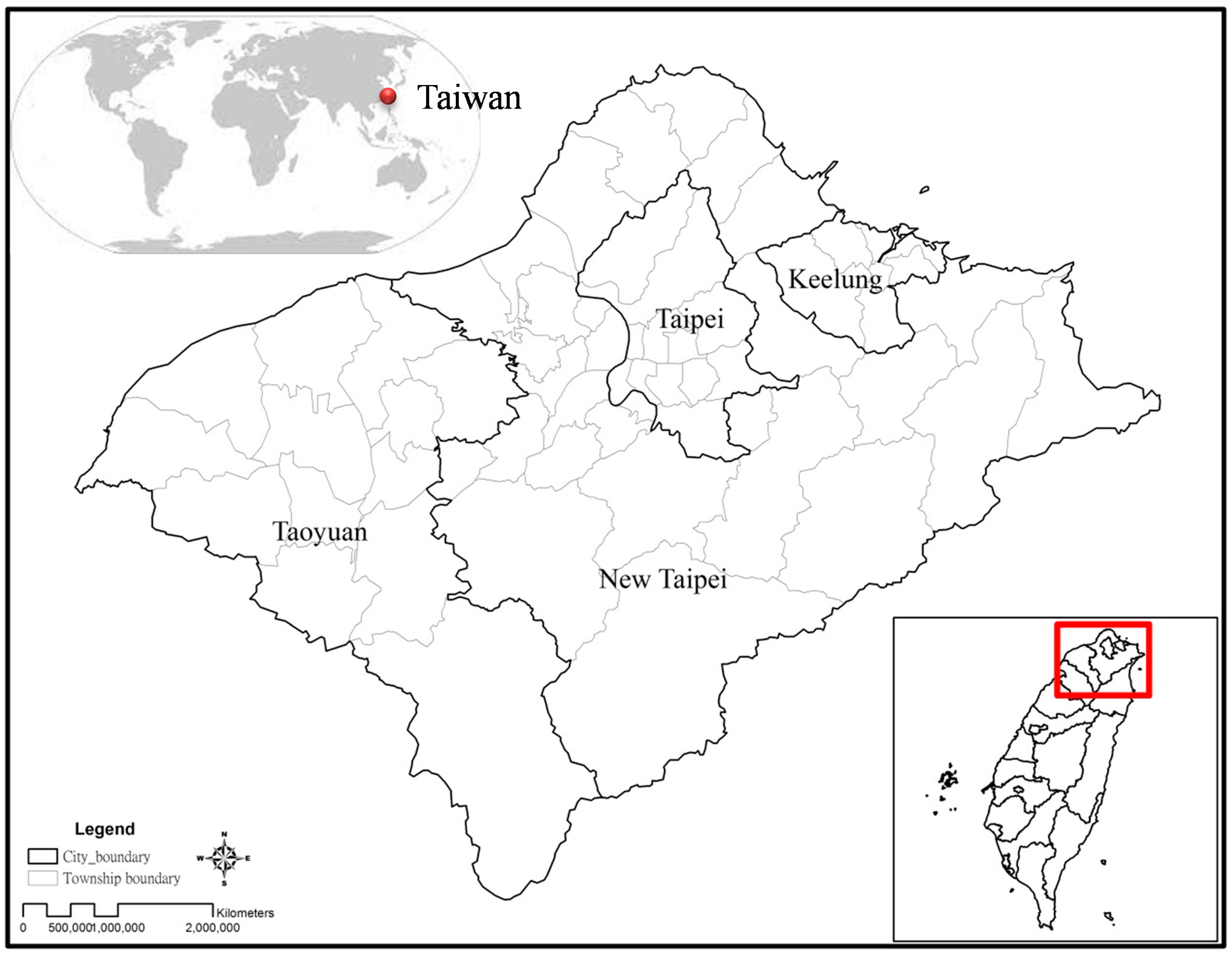
Cities from the Taipei metropolitan area—Taipei, New Taipei, Keelung, and Taoyuan were selected as study areas for this analysis (
Figure 1) because they represent the largest populations in Taiwan. As a result of the significant domestic migration to these cities, they offer important illustrations of density and mixed land use.
The general socioeconomic trend of Taipei has created a polycentric pattern, with the wealthier residents located inside the city. Situated near Taipei, Keelung, and Taoyuan, the city of New Taipei has the largest population. New Taipei has long been recognized as a suburb of Taipei. The urbanized core of New Taipei is concentrated around the boundary between Taipei and New Taipei, while lower population densities and a vegetated area characterize the outskirts of the city.
Taoyuan, which has the largest international airport in Taiwan, developed from a satellite city of the Taipei metropolitan area into the fourth-largest city in Taiwan. Due to its proximity and convenience to New Taipei and Taipei City, Taoyuan County attracts the most immigration in Taiwan. Keelung has the second-largest seaport. Currently, Keelung is a satellite city of the Taipei metropolitan area.
The township is the basic unit in the following spatial analyses. A township refers to a governmental unit of variable geographic size and shape contained within a city or county. There are 12 townships within Taipei, 29 townships within New Taipei, 13 townships within Taoyuan, and seven townships within Keelung. Therefore, there are 61 townships within the study area.
Figure 1.
Location of study area within Taiwan and the township boundaries.
Figure 1.
Location of study area within Taiwan and the township boundaries.
2.2. Dependent and Exploratory Variable
In order to detect the spatial heterogeneity of the urban compaction factors influencing UGS, this study uses urban green space as a dependent variable and extends Burton’s research [
24] by treating density and mixed land use as independent variables (see
Table 1). When variable data were unavailable, this paper refers to similar data obtained from other studies. The principles by which such data were chosen include whether the data are representative (relative to previous research), obtainable, and consistent with Taiwanese urban features. The variables of high density include building density, residential density, and population density. The variables of mixed land use include facility supply, vertical mixed use, and horizontal mixed use.
Table 1.
Variables in the ordinary least square (OLS) and geographically-weighted regressions (GWR) model.
Table 1.
Variables in the ordinary least square (OLS) and geographically-weighted regressions (GWR) model.
| Variables | Descriptions | Resource |
|---|
| Dependent variable | | |
| Urban green space | Area of park, green area, square, and sport fields in the land use investigation achievements of 2006 | National Land Surveying and Mapping Center * |
| Explanatory variable | | |
| Population density | Population density of each township in 2006 | Urban and Regional Development Statistics |
| Building density | Built environments (including residential, commercial, industrial, and public buildings) and households in 2006 | National Land Surveying and Mapping Center, the Census Administration |
| Sub-core population density | Population density of the sub-core area of each township | Urban and Regional Development Statistics |
| Residential density | Ratio of residential land use and residents | National Land Surveying and Mapping Center, the Census Administration |
| Facilities | Ratio of facilities (including post office, gas station, schools etc.) and residential land use | National Land Surveying and Mapping Center |
| Employment | Ratio of local employment and residents in 2006 | Commerce and Service Census |
| Built environment | Ratio of built environments (including residential, commercial, and industrial land uses) | National Land Surveying and Mapping Center |
2.3. Geographically-Weighted Regression
Conventional global regression models, such as Ordinary Least Squares (OLS), are one of the major techniques used to analyze data and form the basis of many other techniques. OLS regression is particularly powerful as it relatively easy to also check the model assumption such as linearity, constant variance, and the effect of outliers using simple graphical methods. Generally, it is an approach to fitting a model to the observed data [
29,
30,
31].
Conventional global regression models ignore all underlying spatial variability and summarize statistics across an entire area. The hypothesis of spatial stationarity in a relationship may limit one’s descriptive and predictive utilities when considering urban areas [
32,
33]. In fact, many processes are spatially non-stationary and produce different responses across the study area [
28].
Spatial statistics are often applied to analyses to clarify their comparisons. GWR is prone to spatial autocorrelation among variables and is an increasingly popular method of analyzing spatially dependent relationships in urban geographic analyses [
34,
35]. This study employed GWR to identify the spatial relationships between UGS and the degree of urban compaction within the study area. The GWR model is expressed as follows:
where
denotes the coordinate location of each observation i in a space,
and
are parameters to be estimated, and
is the random error term at unit i. The weight assigned to each observation is based on a distance-decay function centered upon observation I [
36].
Bandwidth selection is another essential component of the GWR methodology. Two measures of bandwidth are available in GWR: a fixed-distance kernel and an adaptive kernel. A fixed-distance kernel applies to a constant radius centered upon each observation. An adaptive kernel selects a constant number of neighbors without considering distance. Due to the wide range of township sizes—the smallest township size is 4 km
2, and the largest 351 km
2—such a discrepancy discourages the use of a fixed-distance kernel. Thus, applying an adaptive bandwidth is consistent with reality. Here this paper applies the adaptive Gaussian kernel:
where
dij denotes the spatial distance between two observations, and b denotes the bandwidth that are variables.
This study must assess the number of neighbors after selecting the appropriate bandwidth type through measures such as cross-validation (CV) and the Akaike information criterion (AIC) to determine an optimal value for the bandwidth. The appropriate bandwidth for the analysis is not determined due to the township size in our study area. Therefore, this study examines and compares both the manual (nearest neighbors) and AIC approaches to determine the bandwidth. The AIC is based on information entropy and is applied to test the goodness of fit of the model. The definition of the AIC is as follows:
where k denotes the number of parameters, and L is the likelihood function for the estimated model.
AICc is the AIC with a correction for finite sample sizes:
where n denotes the observation size.
Due to the finite number of observation units, this study compares the manual (using 15, 30, and 45 neighbors) and AIC approaches to determine the bandwidth values. Since 30 neighbors demonstrate a greater range of
R2 adjusted, and a lower range of AICc (
Table 2), the manual approach will be adopted for further GWR model analyses.
Table 2.
Geographically-weighted regression (GWR) for manual bandwidth and Akaike information criterion (AIC) bandwidth selection.
Table 2.
Geographically-weighted regression (GWR) for manual bandwidth and Akaike information criterion (AIC) bandwidth selection.
| | Manual bandwidth selection | AIC bandwidth selection |
|---|
| Number of neighbors | 15 | 30 | 45 | 61 |
| R2 | 0.827 | 0.715 | 0.537 | 0.399 |
| R2 Adjusted | 0.132 | 0.404 | 0.299 | 0.249 |
| AICc | −13.317 | 1771.662 | 1806.381 | 1798.848 |
Finally, it is necessary to test the results of the GWR models. Monte Carlo simulations and spatial autocorrelation are commonly used for this purpose [
37]. This study utilizes Monte Carlo simulations to generate random variables; furthermore, this study compares the original model with the simulated model to demonstrate spatial non-stationarity.
3. Results
3.1. Comparison of OLS and GWR
This study compares adjusted
R2 and AICc from OLS and GWR to determine whether the GWR model is better than the OLS. A larger adjusted
R2 (value varies from 0 to 1) and the lower AICc indicate a better model performance. The
R2 value reached from 0.01 for the relationships between UGS and the disequilibrium ratio between residential and commercial to 0.25 for that between UGS and the sub-core population density according to the global regression analysis (
Table 3).
Table 3.
Akaike information criterion correction (AICc) and adjusted R2 comparison.
Table 3.
Akaike information criterion correction (AICc) and adjusted R2 comparison.
| Urban compaction | | OLS | GWR |
|---|
| Coefficient | AICc | Adjusted R2 | AICc | Adjusted R2 | Monte Carlo test for the significance of parameters |
|---|
| slope | intercept |
|---|
| Population density | 244,108 | 1795.416 | 0.142 | 1792.431 | 0.283 | p = 0.29 | p <0.001 |
| Building density | 291,731 | 1790.244 | 0.212 | 1786.859 | 0.344 | p = 0.24 | p < 0.001 |
| Sub-core population density | 327,911 | 1787.188 | 0.25 | 1784.967 | 0.368 | p = 0.84 | p < 0.001 |
| Residential density | 216,943 | 1797.639 | 0.11 | 1794.311 | 0.263 | p = 0.62 | p < 0.001 |
| Facilities | 117,177 | 1803.626 | 0.018 | 1797.451 | 0.215 | p = 0.61 | p < 0.001 |
| Employment | −85,429 | 1804.125 | 0.01 | 1791.8 | 0.288 | p = 0.8 | p < 0.001 |
| Built environment | 232,683 | 1796.471 | 0.127 | 1795.4 | 0.251 | p = 0.46 | p < 0.001 |
The R2 value reached from 0.215 for the relationships with facilities to 0.368 for the sub-core population density; in this area, GWR demonstrates an improvement over OLS. The GWR model had a higher R2 and a lower AICc than the OLS model, which indicates a closer interpretation of the real world. The Monte Carlo testing results revealed that the relationships between the degree of urban compaction and UGS are non-stationary, and significant non-stationarity came from the intercept parameters.
In addition, this study applied the ANOVA test to evaluate whether the GWR model improves upon the OLS model. The results (
Table 4) reveal that the GWR model demonstrates an improvement over the OLS model in the two residuals.
Table 4.
Contrast between ordinary least square (OLS) and geographically weighted regressions (GWR).
Table 4.
Contrast between ordinary least square (OLS) and geographically weighted regressions (GWR).
| | SS | DF | F |
|---|
| OLS residuals | 1.52 × 10¹³ | 8 | |
| GWR improvement | 1.99 × 10¹² | 6.04 | |
| GWR Residuals | 1.32 × 10¹³ | 46.96 | 1.16 |
3.2. The Scale Dependence of Spatial Non-Stationarity
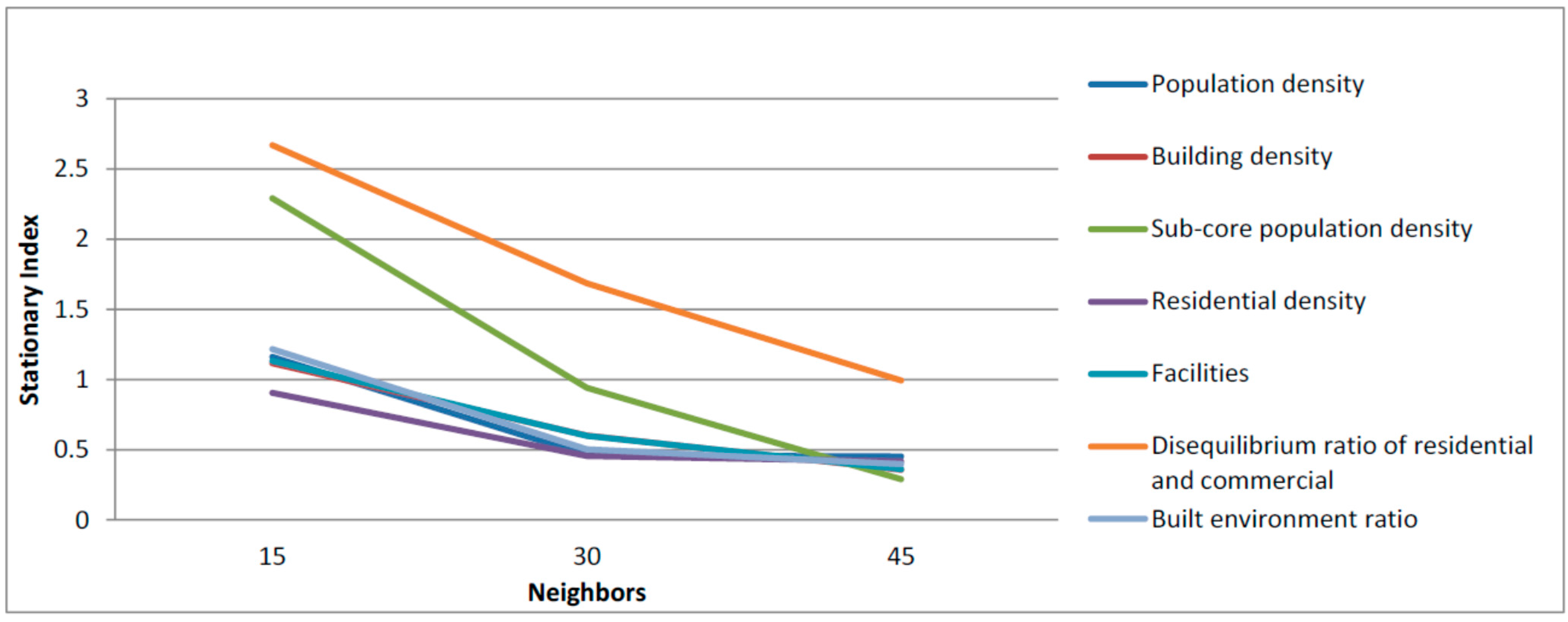
The stationarity index is the ratio between the interquartile range of the regression coefficient from GWR and twice the standard error from the conventional regression analysis. Values less than one indicate stationarity at the spatial scale [
38]. The stationarity index declines rapidly, particularly for the variable sub-core population density. In addition, the stationarity index declines by less than one for most variables at a spatial scale of 30 neighbors, which indicates that 30 neighbors is the significant operating scale of each variable (
Figure 2). The sub-core population density and the disequilibrium ratio between residential and commercial share a significant decreasing gradient and a larger stationarity index, which indicates that the sub-core population and the disequilibrium between residential and commercial influence UGS.
In summary, significant spatial scale dependence occurs in the relationships between UGS and the degree of urban compaction. At a spatial scale of 30 neighbors, the stationarity index of most variables is less than 1 and gradually flattens; this can be considered the intrinsic scale between the relationships. Thus, 30 neighbors is the acceptable bandwidth to model the relationship between UGS and the related urban compaction degree variables in this study.
Figure 2.
Multi-scale stationary index for urban compaction degree variables.
Figure 2.
Multi-scale stationary index for urban compaction degree variables.
3.3. Spatial Heterogeneity of Relationships between UGS and Urban Compaction Degree Variables
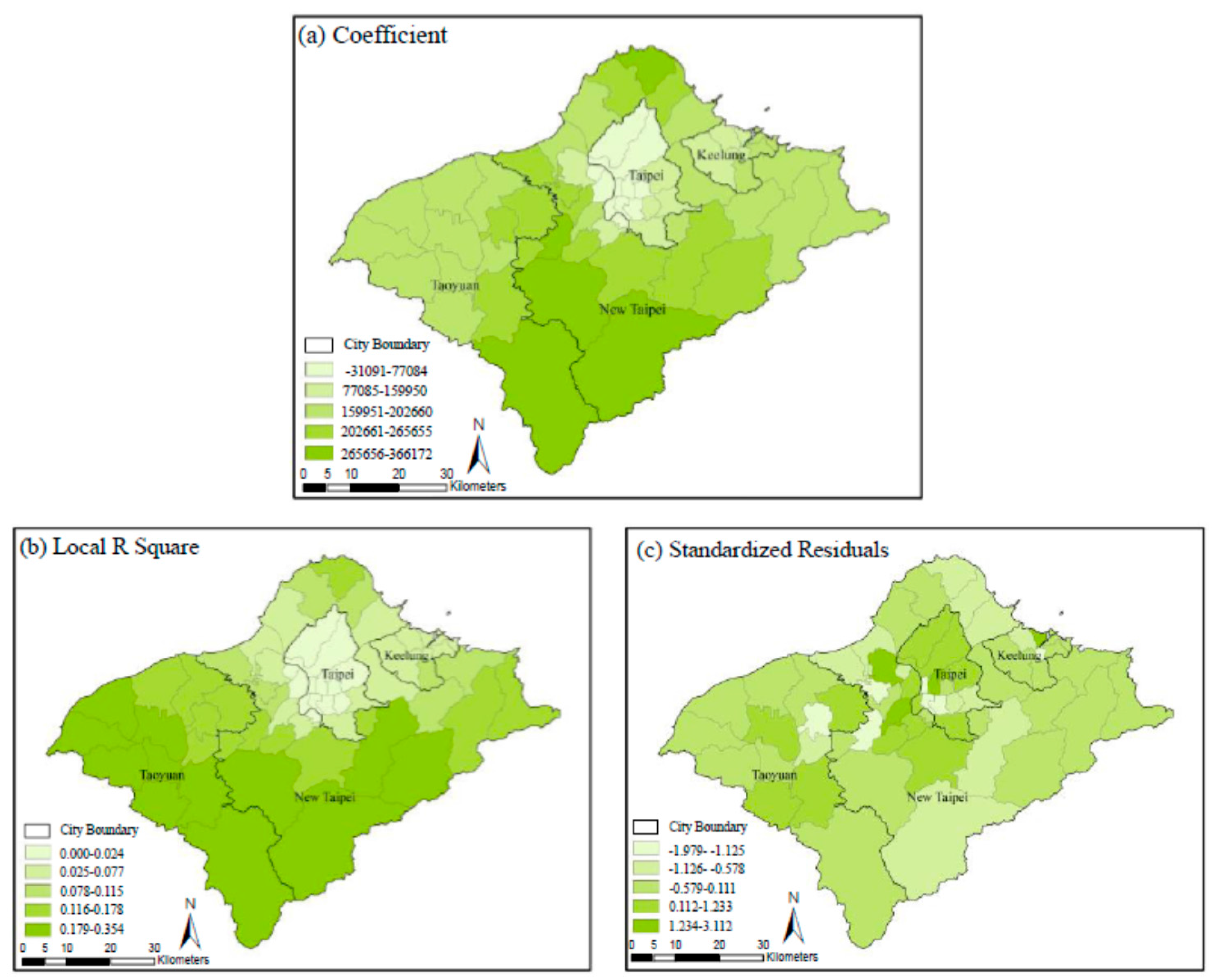
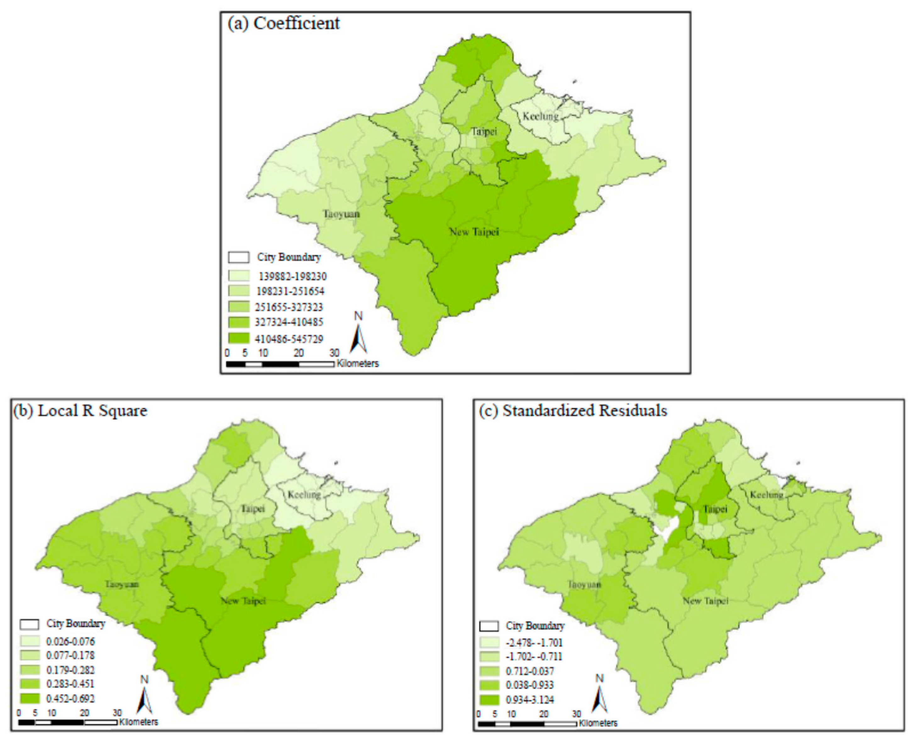
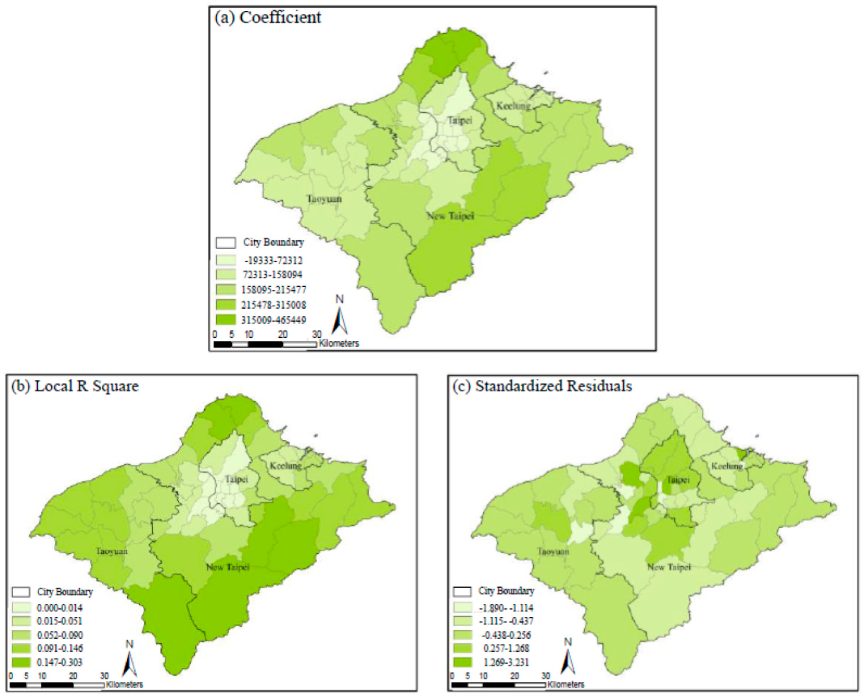
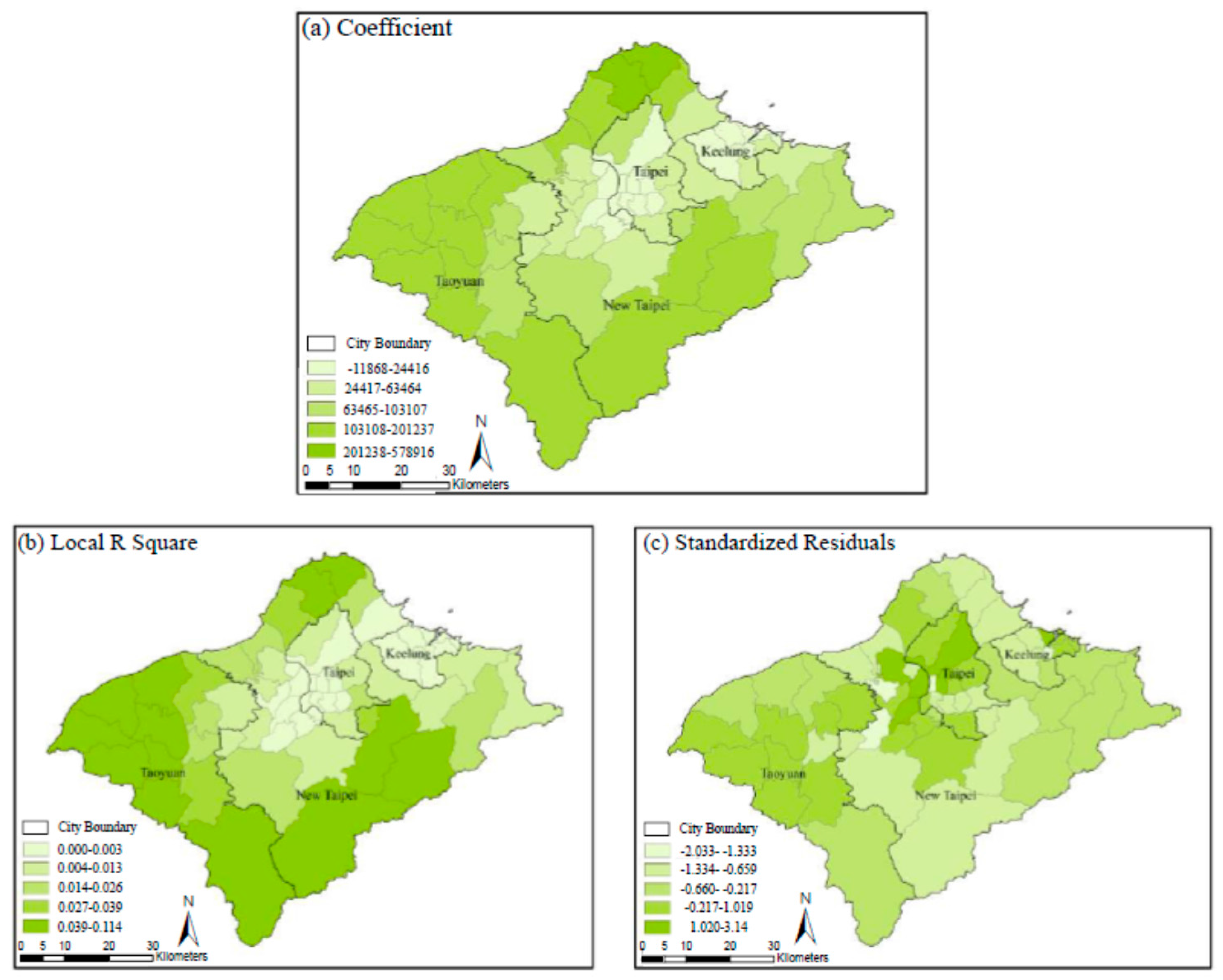
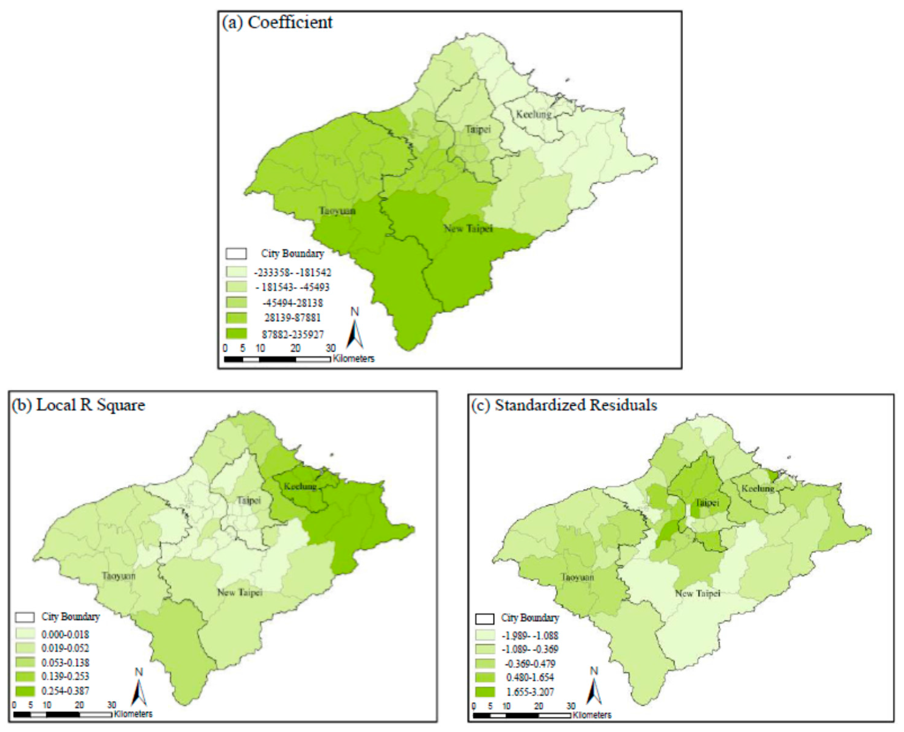
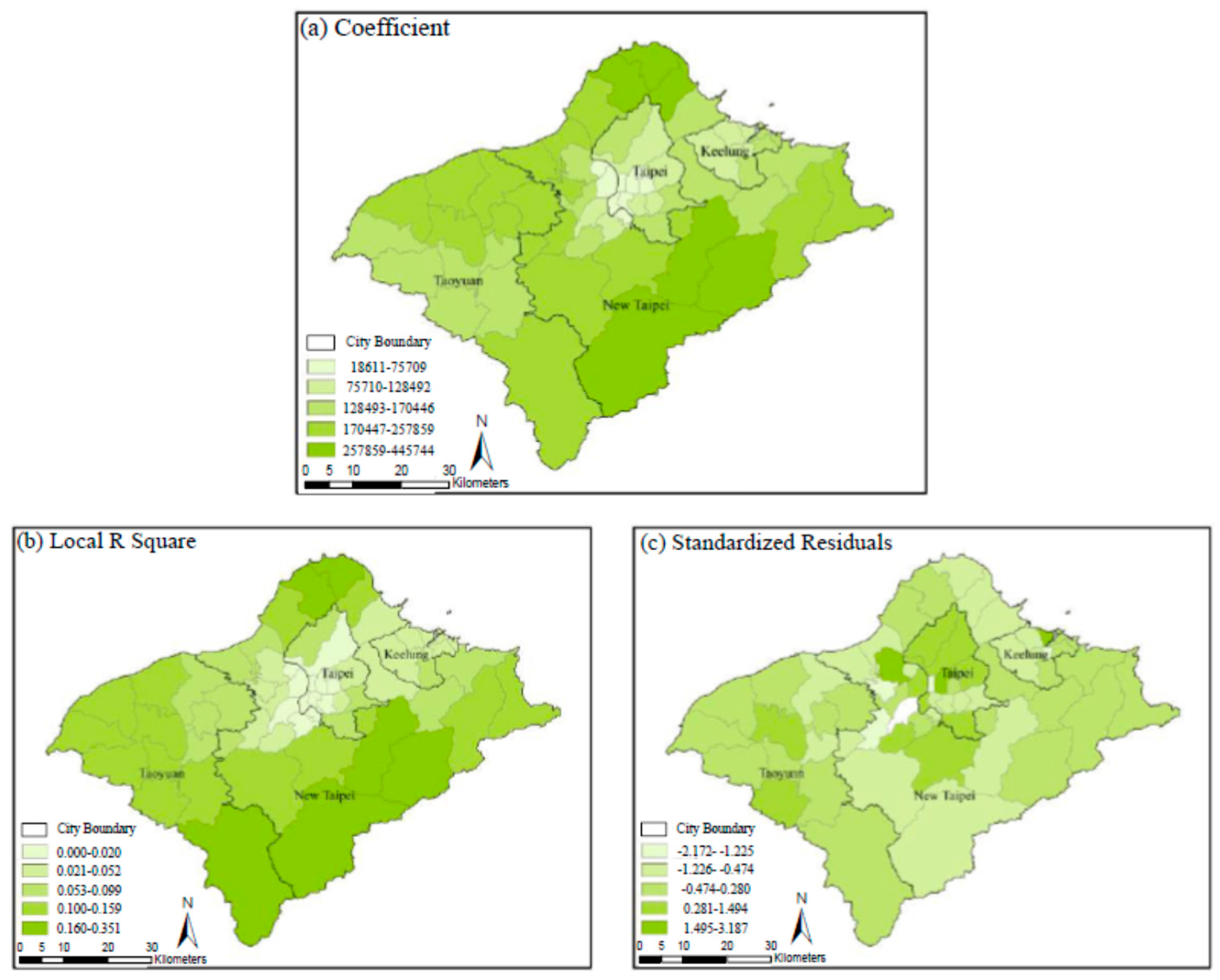
This study detects the varying spatial relationships between UGS and the urban compaction degree variables based on slope parameters (β coefficients), local R2, and standardized residuals from GWR models. The coefficient represents the strength and type of relationship between the urban compaction degree variables and UGS. The local R2, ranging from 0 to 1, measures the fitness of the model. The standardized residual indicates the standard deviation between the observed and the predicted values.
The results of the coefficient, local
R2, and standardized residuals generated from the GWR model for UGS and for the urban compaction degree variables (
Figure 6). Most urban compaction degree indicators share similar patterns, such as population density, building density, sub-core population density, residential density, facilities, and built environment ratio. Significant positive correlations are observed in the southern area, according to parameter estimates and local
R2 (
Figure 3,
Figure 4,
Figure 5,
Figure 6,
Figure 7,
Figure 8 and
Figure 9). However, the positive weights of the standardized residuals reflect over-prediction in the central study area, which is a relatively random pattern compared with local
R2 and parameter estimates.
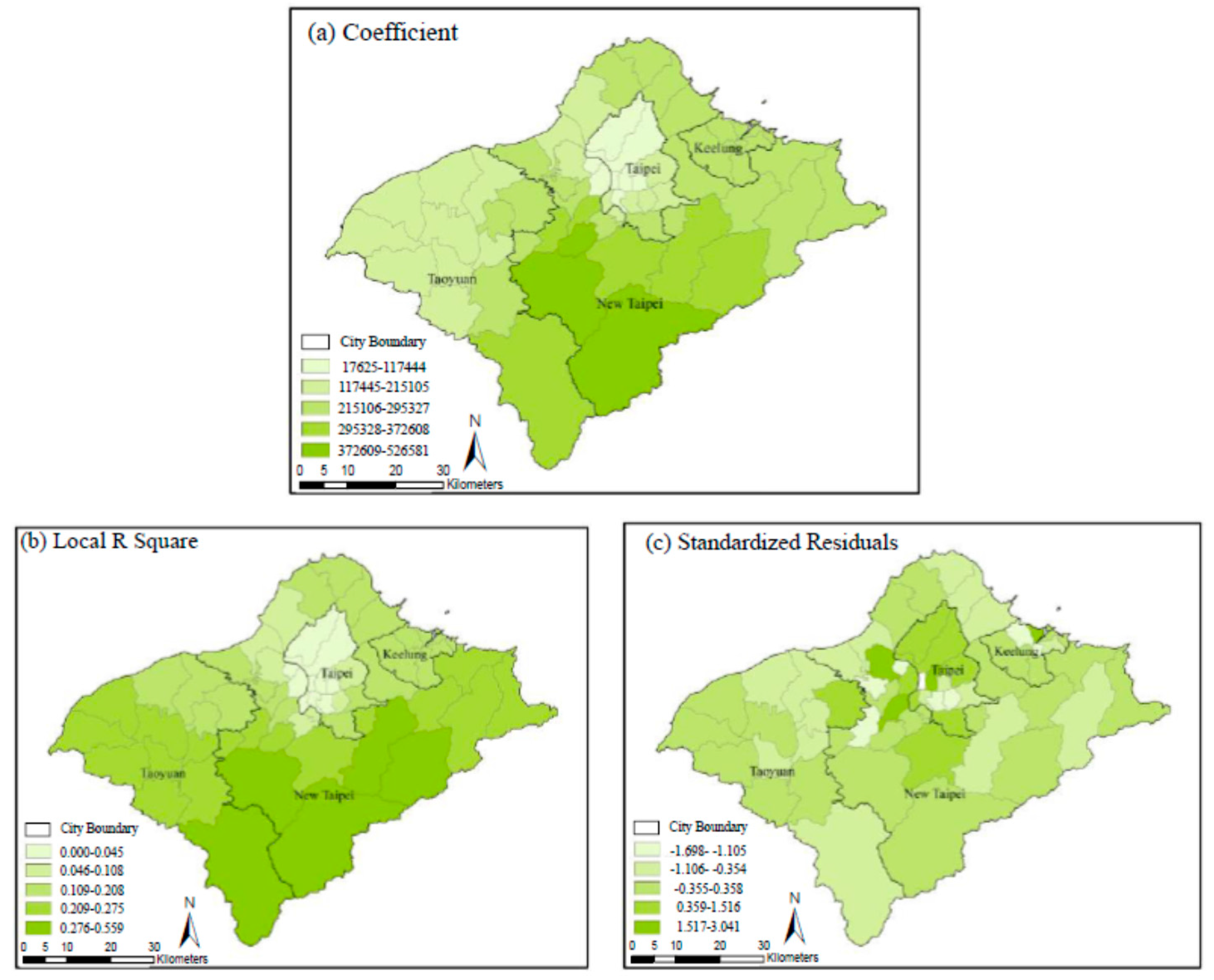
According to the GWR results, significant spatial non-stationarity is observed in the local R2 and parameter estimates in the maps of the subject area. Strong positive relationships are clustered in the southern and northern areas. The tendency of the disequilibrium ratio between residential and commercial exhibits significant divergence compared with the other variables. Because the other variables have an acceptable local R2, different variables with consistent tendencies might be referred in further analyses. According to the results of the parameters and the local R2, the relationships between UGS and the degree of urban compaction can be divided into three types, including superior UGS allocation, insufficient UGS allocation and moderate UGS allocation.
3.3.1. Superior UGS Allocation
Two separate areas, the southern and northern, can be considered superior UGS allocations. The southern area has both a higher local R2 and parameters among the compaction degree variables of population density, building density, sub-core population density, and built environment ratio. The northern area has a moderate local R2 and higher parameters among the compaction degree variables of sub-core population density, residential density, facilities, and built environment ratio. The superior UGS allocation in these two areas can be understood as a paradigm of compact city, exhibiting compact development of both the population and buildings with high UGS allocations.
3.3.2. Insufficient UGS Allocation
The central area (Taipei City) is an example of an insufficient UGS allocation; all of its compaction degree variables exhibit lower parameters. The results of this study indicate that either the control population or the building density or the increment of UGS amount is necessary to be taken into account in future urban planning. An insufficient UGS allocation combined with a dense population and a high building density may not appropriate to be a livable compact city.
3.3.3. Moderate UGS Allocation
Moderate local R2 and parameters appear in the eastern and western areas, which indicate a moderate UGS allocation.
Figure 3.
β coefficients, local R2, and standardized residuals of population density.
Figure 3.
β coefficients, local R2, and standardized residuals of population density.
Figure 4.
β coefficients, local R2, and standardized residuals of building density.
Figure 4.
β coefficients, local R2, and standardized residuals of building density.
Figure 5.
β coefficients, local R2, and standardized residuals of sub-core population density.
Figure 5.
β coefficients, local R2, and standardized residuals of sub-core population density.
Figure 6.
β coefficients, local R2, and standardized residuals of residential density.
Figure 6.
β coefficients, local R2, and standardized residuals of residential density.
Figure 7.
β coefficients, local R2, and standardized residuals of facilities.
Figure 7.
β coefficients, local R2, and standardized residuals of facilities.
Figure 8.
β coefficients, local R2, and standardized residuals of employment.
Figure 8.
β coefficients, local R2, and standardized residuals of employment.
Figure 9.
β coefficients, local R2, and standardized residuals of built environment.
Figure 9.
β coefficients, local R2, and standardized residuals of built environment.
4. Discussion
Current trends have inspired compact cities to examine their own conditions while engaging in the following activities: increasing the density of highly developed areas; intensifying urban activities across economic, social, and cultural realms [
39], and manipulating urban settlements [
40]. For example, higher densities lead to greater traffic congestion and reduced fuel efficiency [
6]. Furthermore, when more residents populate an urban area, land prices inevitably rises, and the amount of space available for greenery shrinks [
41]. In fact, having UGS nearby typically extends the living space and offers a connection with nature; it can also be strategically important because it provides a cooling effect and further maintains a high quality of life [
11,
17,
19,
37,
42]. In addition, UGS not only has directly impacts on physical activity but also on raising the surrounding land value for the improvement of living environment [
16,
23].
Therefore, examining spatial variation in the relationships between the degree of urban compaction and UGS provides an opportunity to examine the current compact city paradigm at a time when the compact city concept is receiving an increasing amount of attention for use in cities with limited developmental land and vulnerable environments. The overall conclusions of such studies should be considered in future UGS allocation strategies to ensure the equal distribution of environmental benefits. Their application to global and local spatial assessments fosters the analysis of various geographic trends between vegetation and urban environments [
43]. The results of both the global and local UGS assessments provide a series of statistics for use in analyses of spatial features between urban compaction degree factors and UGS. In this article, this study applied OLS as the global method and GWR as the local method. The coefficients of OLS indicate the general tendency of compact city factors influencing UGS, e.g., a higher degree of urban compaction, leads to higher UGS (see
Table 3). However, the OLS results appear to be unable to show spatial non-stationarity across cities [
38,
41,
44,
45].
Since this study maintained the feature of non-stationarity in the relationships between the degree of urban compaction and UGS, this study examined spatial non-stationarity on a multi-scale measure. The stationarity index is less than one for most predictors, while the spatial scale is 30 neighbors, indicating that 30 neighbors is the significant operating scale among the variables. Thus, at a spatial scale of 30 neighbors, the stationarity index of most variables is less than one and gradually flattens, which can be considered the intrinsic scale between the relationships. Furthermore, the application of the GWR model resulted in the observation of spatial non-stationarity in highly populated cities in Taiwan. Spatial non-stationarity associated with UGS was observed with the urban compaction degree variables related to high density and mixed land use. Significant positive correlations among the urban compaction degree variables were observed in the southern area, whereas negative correlations were concentrated in the central area.
Maps summarizing the GWR results between the degree of urban compaction and UGS demonstrate that there is significantly insufficient UGS allocation in the central area, which consists mainly of Taipei City and thus contains the highest population density and building densities within the city region. There is an urgent need to implement UGS allocation in such townships. Townships with higher parameters contain UGS levels that better meet the needs of their residents. However, the accessibility and availability of UGS were not considered in this study. Applying the GWR method to analyze the relationships between the degree of urban compaction and UGS provides a tool to help explore geographic trends and to discuss whether the compact city model benefits overall livability, increasing emphasis on the quality of the urban environment as a living space for people. Therefore, it is necessary to monitor urban development to assure cities are sustainable in a wide range of social, economic, and environmental needs to be satisfied [
46].


