A Stochastic Programming Approach with Improved Multi-Criteria Scenario-Based Solution Method for Sustainable Reverse Logistics Design of Waste Electrical and Electronic Equipment (WEEE)

Abstract

Today, the increased public concern about sustainable development and more stringent environmental regulations have become important driving forces for value recovery from end-of-life and end-of use products through reverse logistics. Waste electrical and electronic equipment (WEEE) contains both valuable components that need to be recycled and hazardous substances that have to be properly treated or disposed of, so the design of a reverse logistics system for sustainable treatment of WEEE is of paramount importance. This paper presents a stochastic mixed integer programming model for designing and planning a generic multi-source, multi-echelon, capacitated, and sustainable reverse logistics network for WEEE management under uncertainty. The model takes into account both economic efficiency and environmental impacts in decision-making, and the environmental impacts are evaluated in terms of carbon emissions. A multi-criteria two-stage scenario-based solution method is employed and further developed in this study for generating the optimal solution for the stochastic optimization problem. The proposed model and solution method are validated through a numerical experiment and sensitivity analyses presented later in this paper, and an analysis of the results is also given to provide a deep managerial insight into the application of the proposed stochastic optimization model.

1. Introduction

Today, with rapid technological advancement and economic development, the manufacturing of electrical and electronic products has become one of the most rapidly developing and growing industries [1,2,3]. This growth has significantly altered the lifestyle and consumption pattern of human beings [2,4]. On the one hand, more and more innovative, well-designed, and multi-functional electrical and electronic products are introduced, usually at an attractive price, to make our lives better and more convenient. On the other hand, customers’ pursuit of a better lifestyle also leads to an increasingly shortened product life cycle, particularly for electrical and electronic products, which results in rapidly increased generation of Waste Electrical and Electronic Equipment (WEEE) all over the globe. The annual increase of WEEE generation has reached approximately 5% since 2005 [5], which is almost three times higher than the increase of other waste [6]. In 2012, the WEEE generation in the world is approximately 49 million metric tons [7], and the three largest markets for electrical and electronic products (the United States, China, and the European Union) together contribute 54.1% of the total amount of WEEE generation [7]. The rapid growth of WEEE generation has become a significant challenge due to the lack of formal recycling and recovery channels [8], and an earlier study has revealed that only 1.5 million metric tons of WEEE in Europe were recycled through formal take-back schemes [4]. A recent report released by the Countering WEEE Illegal Trade (CWIT) project [9] reveals that the total amount of WEEE generated in Europe was 9.45 million tons in 2012, of which only 35% was recycled and treated through the formal recycling system; the other 65% was exported (15.8%), recycled through non-compliant conditions in Europe (33.4%), scavenged for valuable parts (7.9%), or sent to landfill (7.9%). According to the report [9], due to the mismanagement of discarded electronics in Europe, there is still a large amount of WEEE sent to and recycled in developing countries, e.g., China, Vietnam, etc., where, unlike in developed countries, most of the WEEE are reused and recycled under lower standards through low-tech companies or disposed of in landfills [10]. From a global perspective, this will reduce the economic sustainability (waste of recyclable and valuable resources [9]), environmental sustainability (environmental pollution [9]), as well as social sustainability (risk to workers’ health [9,11]) of modern society. Therefore, more effort should be directed to providing guidelines and support systems for decision-makers in order to enhance formal recycling systems for sustainable management of WEEE, so more WEEE can be recycled and treated in an economically efficient, environmentally sound, and socially responsible manner.

Reverse logistics is considered as one of the most effective solutions for value recovery from end-of-life and end-of-use products [12]. Reverse logistics is defined as the process starting from the customer towards the raw material supplier, and it aims at—through planning, operating, and managing efficient material flow, information flow, and cash flow—recovering the remaining value from end-of-life and end-of-use products and disposing of waste in a proper way [13]. Due to public concern about sustainable development, reverse logistics activities have been extensively focused in the past two decades [14,15,16,17]. Compared with other used products, the reverse logistics design for WEEE management is more complicated, because WEEE contains not only renewable materials and components, e.g., glass, plastics, and precious metals [8], which need to be reused and recycled, but also hazardous substances, e.g., nickel, lead, and mercury [18,19], which have to be properly treated or disposed of in order to minimize the risk to people’s health and the environment. Therefore, the development of advanced tools for complex decision-making problems related to the design and planning of a sustainable reverse logistics system for WEEE is of paramount importance.

In order to have an overview of the theoretical development and practical implementation, this paper reviews some of previous studies regarding the reverse logistics of WEEE, and an extensive literature review of the decision models of WEEE management is provided by Xavier and Adenso-Diaz [20]. Walther and Spengler [21] formulate a linear programming for allocating WEEE to different facilities in an optimal fashion, and the model is used to estimate the influence of EU WEEE Directive on reverse logistics in Germany. Dat et al. [22] introduce a mixed integer programming for minimizing the total costs of reverse logistics of WEEE, considering the costs of collection, transportation, treatment, and income from the sale of recycled products. Gomes et al. [23] develop a generic mixed integer program for multi-product reverse logistics network design of WEEE; the model determines the best locations of collection and sorting centers and the material flows in each route.

Kilic et al. [24] propose a mixed integer programming for designing the optimal reverse logistics network structure of WEEE. The model is solved with CPLEX and 10 scenarios with different collection requirements are tested and discussed in this paper. Quariguasi Frota Neto et al. [25] develop a mathematical model for eco-efficient lot size problem with remanufacturing options, and the sustainable issue is formulated by Cumulative Energy Demand (CED). Alumur et al. [26] formulate a multi-commodity and multi-period mixed integer programming for reverse logistics network design of WEEE. The model maximizes the profit generated from the reverse logistics activities and is validated through real-world case studies of tumble dryers and washing machines in Germany. Furthermore, the multi-period formulation provides scope for future improvement of the configuration of reverse logistics systems.

Grunow and Gobbi [27] develop a decision support model for assigning different municipalities to different waste management schemes in an efficient and fair manner. Achillas et al. [4] formulate a location–allocation model for regulators and policy-makers for the optimal design of reverse logistics network of WEEE. Capraz et al. [28] propose a mixed integer linear programming for decision-making of recycling companies of WEEE, and the model simultaneously determines the maximal bid price offered by the company and the optimal operational plan of the plant. Liu et al. [29] propose a quality-based price competition model for assessing the performance of both formal and informal recycling channels of WEEE. The study reveals that the quality is the most important influencing factor for WEEE recycling, and high-quality WEEE are preferred by both formal and informal markets. Furthermore, the informal recycling market is of great advantage when the quality of WEEE is high and the formal recycling channel is not heavily subsidized by the government.

Manzini and Bortolini [30] introduce a two-stage decision-aided system for both strategic and operational decision-making of reverse logistics of WEEE. The optimal location–allocation plan is first determined by a mixed integer programming, and a heuristic algorithm is then applied to solve the vehicle routing problem. Yao et al. [31] develop a quadratic optimization model to determine the minimum number of transit sites for reverse logistics of WEEE, and a modified ant colony algorithm is then applied for routing the collection vehicles. Tsai and Hung [32] propose a two-stage decision framework for planning a treatment and recycling system for WEEE. The waste treatment companies are first selected at the treatment stage, and a linear programming is formulated in recycling stage for maximizing the profit generated from WEEE recycling. Mar-Ortiz et al. [33] formulate an integer programming model for the vehicle routing problem of WEEE, and two computational algorithms, a GRASP-based algorithm and a saving-based algorithm, are employed and compared in resolving the complex optimization problem.

Shokohyar and Mansour [34] develop a simulation- and optimization-based framework for sustainable planning of the reverse logistics network of WEEE. Different network configurations are first tested in the simulation stage through the professional simulation software Arena, and then, in the optimization stage, a multi-objective model is formulated to determine the value of three objective functions: profit, environmental influence, and social sustainability. Yu and Solvang [2] formulate a bi-objective mixed integer programming for sustainable reverse logistics design of WEEE. The model simultaneously balances the overall system costs and carbon emissions, and the two objective functions are combined with the weighted sum method.

The literature review shows that most previous decision models for reverse logistics system design of WEEE management are deterministic models without consideration of the uncertainties of input parameters. To our knowledge, the only exemption is provided by Ayvaz et al. [35]. In this study, a two-stage stochastic programming model is formulated for maximizing the profit of the reverse logistics system for WEEE management under uncertainty, and the sample average approximation method is employed to resolve the stochastic optimization problem. Reverse logistics is characterized by a high level of uncertainty [36], so it is important to consider the uncertain issues in reverse logistics system design of WEEE management. Due to the lack of uncertainty in previous models, this paper aims at filling the literature gap by providing a new stochastic programming model for reverse logistics network design of WEEE management; furthermore, the model not only considers the economic performance but also accounts for the environmental sustainability of the reverse logistics system for WEEE. In this study, the environmental sustainability is evaluated by carbon footprint, and a multi-criteria scenario-based solution method developed by Soleimani et al. [37] is employed to resolve the stochastic optimization problem. The original solution method is only capable to resolve the min-max and max-min stochastic optimization problems; furthermore, the managerial meaning of the solution method is unclear. The multi-criteria scenario-based solution method is further improved and developed in this paper so that all types of stochastic optimization problems (min-max, max-min, min-min, and max-max) can be solved and a clear managerial meaning can also be interpreted from the result.

The remainder of the paper is organized as follows. Section 2 provides the problem statement and formulates the stochastic mixed integer programming for the design of a sustainable reverse logistics system for WEEE management under uncertainty. Section 3 introduces the two-stage multi-criteria scenario-based solution method for stochastic optimization problem, and the difference between the improved solution method and the original solution method is presented in this section. Section 4 presents a numerical experiment in order to illustrate the application of the proposed model in the decision-making of reverse logistics system design of WEEE. Section 5 provides sensitivity analyses in order to validate the model with changing parameters. Section 6 concludes the paper and provides suggestions for future research.

2. Problem Statement and Modeling

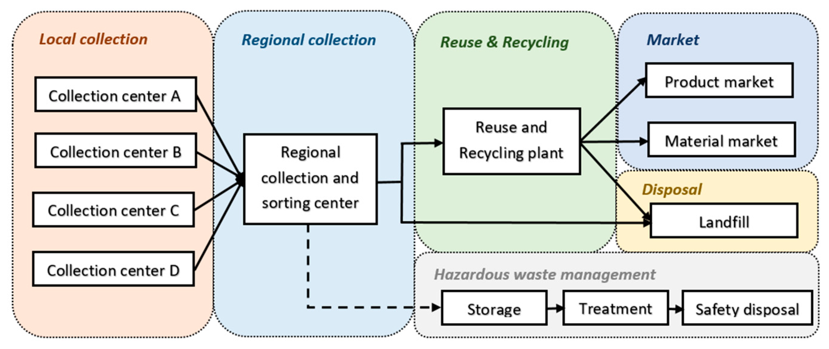
Figure 1 illustrates the reverse logistics system for WEEE management. The end-of-use and end-of-life electrical and electronic products are first collected at a local WEEE collection center (e.g., retailers of electronic products, supermarkets, public facilities for WEEE collection, etc.), and then will be transported to a regional collection center for preprocessing. At the regional collection center, WEEE are inspected and sorted for further treatment including reuse, recycling, and disposal. It is noteworthy that some electrical and electronic products contain hazardous materials that have to be separated out at this step and sent to specialized hazardous waste treatment plants. The recyclable parts and components from WEEE are sent for reuse and recycling, and the non-recyclable fraction is sent to an incineration plant or a landfill for proper disposal. The recycled products from WEEE will be sold at primary or secondary markets, and the recycled components will be sold to manufacturers of electrical and electronic products for material recovery.

The proposed mathematical model aims at determining the optimal configuration of the reverse logistics system for WEEE, which includes the locations of regional collection centers and recycling plants, and the material flows between different facilities. Due to the uncertainty, the generation of WEEE, price of recycled products, and price of recycled materials are considered to be stochastic parameters, and the different sources of WEEE and the environmental influence are also taken into account in this model. Therefore, the proposed model is a multi-source, multi-echelon, and capacitated stochastic network optimization problem. In this paper, we use the word “product” to differentiate the sources of WEEE.

The assumptions of the model are given as follows:

• The number and locations of local collection centers, product markets, material markets, and disposal facilities are known.
• The potential locations of regional collection centers and recycling plants are known.
• The fixed costs, unit transportation costs, and unit processing costs are known.
• The capacities of new facilities are predetermined.
• The WEEE can be converted at a fixed rate to new products, recycled parts, disposal fractions, and hazardous materials.
• The carbon emissions rate is mainly determined by the size of facility and technology adopted in the treatment and transportation of WEEE.

The sets, parameters, and decision variables are given as follows:

Sets:
C	Set of local collection sites of WEEE, indexed by c
R	Set of potential locations of regional collection centers of WEEE, indexed by r
P	Set of potential locations of recycling plants of WEEE, indexed by p
H	Set of hazardous waste management systems, indexed by h
F	Set of product market, indexed by f
M	Set of material market, indexed by m
D	Set of disposal sites, indexed by d
L	Set of products, indexed by l
S	Set of scenarios, indexed by s
Parameters:
$F{x}_r$	Fixed cost of opening regional collection center at potential location r $\in$ R
$F{x}_p$	Fixed cost of opening recycling plant at potential location p $\in$ P
$C{p}_{rl}$	Unit cost at regional collection center r $\in$ R for processing product l $\in$ L
$C{p}_{pl}$	Unit cost at recycling plant p $\in$ P for processing product l $\in$ L
$C{p}_d$	Unit cost at disposal site d $\in$ D
$C{p}_h$	Unit cost at hazardous waste management system h $\in$ H
$PC{p}_{fl}^s$	Unit price of recycled product l $\in$ L at product market f $\in$ F in scenario s $\in$ S
$PC{m}_{ml}^s$	Unit price of recycled product l $\in$ L at material market m $\in$ M in scenario s $\in$ S
$Ct{r}_{lcr}$	Transportation cost per unit product l $\in$ L from local collection site c $\in$ C to regional collection center r $\in$ R
$Ct{r}_{lrp}$	Transportation cost per unit recyclable fraction of product l $\in$ L from regional collection site r $\in$ R to recycling plant p $\in$ P
$Ct{r}_{lrd}$	Transportation cost per unit disposed fraction of product l $\in$ L from regional collection center r $\in$ R to disposal site d $\in$ D
$Ct{r}_{lrh}$	Transportation cost per unit hazardous fraction of product l $\in$ L from regional collection center r $\in$ R to hazardous waste management system h $\in$ H
$Ct{r}_{lpf}$	Transportation cost per unit recycled fraction of product l $\in$ L from recycling plant p $\in$ P to product market f $\in$ F
$Ct{r}_{lpm}$	Transportation cost per unit recycled fraction of product l $\in$ L from recycling plant p $\in$ P to material market m $\in$ M
$Ct{r}_{lpd}$	Transportation cost per unit disposed fraction of product l $\in$ L from recycling plant p $\in$ P to disposal site d $\in$ D
$\theta$	Unit cost of carbon credit
$C{O}_2^{cap}$	Carbon emissions cap for reverse logistics system for WEEE
$Co{l}_{lc}^s$	Amount of product l $\in$ L collected at local collection site c $\in$ C in scenario s $\in$ S
$Capacit{y}_{rl}$	Capacity of regional collection center r $\in$ R for product l $\in$ L
$Capacit{y}_{pl}$	Capacity of recycling products center p $\in$ P for product l $\in$ L
${\phi }_{lp}$	Recycling fraction of product l $\in$ L
${\phi }_{ld}$	Disposed fraction of product l $\in$ L
${\phi }_{lh}$	Hazardous fraction of product l $\in$ L
$L{m}^{\prime }$	An infinitely large positive number
${\vartheta }_{lf}$	Conversion rate of production l $\in$ L to product market f $\in$ F
${\vartheta }_{lm}$	Conversion rate of production l $\in$ L to material market m $\in$ M
${\vartheta }_{ld}$	Conversion rate of production l $\in$ L to disposal site d $\in$ D
$Em{s}_r$	Carbon emissions per unit capacity for opening a regional collection site r $\in$ R
$Em{s}_p$	Carbon emissions per unit capacity for opening a recycling plant p $\in$ P
$Em{s}_{lcr}$	Carbon emissions for transporting one unit product l $\in$ L from local collection site c $\in$ C to regional collection center r $\in$ R
$Em{s}_{lrp}$	Transportation cost one unit recyclable fraction of product l $\in$ L from regional collection site r $\in$ R to recycling plant p $\in$ P
$Em{s}_{lrd}$	Transportation cost one unit disposed fraction of product l $\in$ L from regional collection center r $\in$ R to disposal site d $\in$ D
$Em{s}_{lrh}$	Transportation cost one unit hazardous fraction of product l $\in$ L from regional collection center r $\in$ R to hazardous waste management system h $\in$ H
$Em{s}_{lpf}$	Transportation cost one unit recycled fraction of product l $\in$ L from recycling plant p $\in$ P to product market f $\in$ F
$Em{s}_{lpm}$	Transportation cost one unit recycled fraction of product l $\in$ L from recycling plant p $\in$ P to material market m $\in$ M
$Em{s}_{lpd}$	Transportation cost one unit disposed fraction of product l $\in$ L from recycling plant p $\in$ P to disposal site d $\in$ D
Decision variables (First-level):
$Y_r^s=\{\begin{array}{c}1\\ 0\end{array}$	Potential location of regional collection center r $\in$ R is selected in scenario s $\in$ S Otherwise
$Y_p^s=\{\begin{array}{c}1\\ 0\end{array}$	Potential location of recycling plant p $\in$ P is selected in scenario s $\in$ S Otherwise
Decision variables (Second-level):
$Q{g}_{rl}^s$	Amount of product l $\in$ L processed at regional collection center r $\in$ R in scenario s $\in$ S
$Q{g}_{pl}^s$	Amount of recycled fraction of product l $\in$ L processed at recycling plant p $\in$ P in scenario s $\in$ S
$Q{g}_d^s$	Amount of disposed fraction of product l $\in$ L processed at disposal site d $\in$ D in scenario s $\in$ S
$Q{g}_h^s$	Amount of hazardous fraction of product l $\in$ L processed at hazardous waste management system h $\in$ H in scenario s $\in$ S
$Q{g}_{fl}^s$	Amount of recycled fraction of product l $\in$ L sold at product market f $\in$ F in scenario s $\in$ S
$Q{g}_{ml}^s$	Amount of recycled fraction of product l $\in$ L sold at material market m $\in$ M in scenario s $\in$ S
$Qt{r}_{lcr}^s$	Amount of product l $\in$ L transported from local collection site c $\in$ C to regional collection center r $\in$ R in scenario s $\in$ S
$Qt{r}_{lrp}^s$	Amount recycled fraction of product l $\in$ L transported from regional collection site r $\in$ R to recycling plant p $\in$ P in scenario s $\in$ S
$Qt{r}_{lrd}^s$	Amount of disposed fraction of product l $\in$ L transported from regional collection center r $\in$ R to disposal site d $\in$ D in scenario s $\in$ S
$Qt{r}_{lrh}^s$	Amount of hazardous fraction of product l $\in$ L transported from regional collection center r $\in$ R to hazardous waste management system h $\in$ H in scenario s $\in$ S
$Qt{r}_{lpf}^s$	Amount of recycled fraction of product l $\in$ L transported from recycling plant p $\in$ P to product market f $\in$ F in scenario s $\in$ S
$Qt{r}_{lpm}^s$	Amount of recycled fraction of product l $\in$ L transported from recycling plant p $\in$ P to material market m $\in$ M in scenario s $\in$ S
$Qt{r}_{lpd}^s$	Amount of disposed fraction product l $\in$ L transported from recycling plant p $\in$ P to disposal site d $\in$ D in scenario s $\in$ S
$C{O}_2^S$	Total amount of carbon emissions from the reverse logistics system for WEEE

The objective function of the mathematical model is given in Equation (1). The first two parts of the equation calculate the facility costs for opening regional collection centers and recycling plants. The third part calculates the processing costs of waste disposal and hazardous waste management. The fourth part determines the profits from selling the recycled products and materials. The fifth, sixth, and seventh parts are the transportation costs of first-level, second-level, and third-level transportation in the reverse logistics system, respectively. The last part calculates the carbon trading costs. Carbon emission is considered as the most important cause of global warming and climate change, so it has been introduced and formulated as the environmental indicator for sustainable supply chain design in many previous studies (e.g., Yu and Solvang [12], Govindan et al. [38], Diabat et al. [39], Kannan et al. [40], Fahimnia et al. [41], and Yu et al. [42]). In this paper, both the economic and environmental sustainability of the reverse logistics of WEEE are taken into account, so the carbon emissions of the reverse logistics activities for WEEE management are quantified by a well-established method: carbon trading [39,40] and combined with the cost objective. Furthermore, it is noteworthy that the model aims at determining the optimal and most reliable and robust solution through all possible scenarios in the reverse logistics design of WEEE.

$$\begin{array}{ll}\mathrm{Min}\mathrm{cost}=& \{{\displaystyle {\displaystyle \sum }_{r\in R}}F{x}_r{Y}_r^s+{\displaystyle {\displaystyle \sum }_{l\in L}}{\displaystyle {\displaystyle \sum }_{r\in R}}C{p}_{rl}Q{p}_{rl}^s\}+\{{\displaystyle {\displaystyle \sum }_{p\in P}}F{x}_p{Y}_r^p+{\displaystyle {\displaystyle \sum }_{l\in L}}{\displaystyle {\displaystyle \sum }_{p\in P}}C{p}_{pl}Q{g}_{pl}^s\}\\ & +\{{\displaystyle {\displaystyle \sum }_{d\in D}}C{p}_{d}Q{g}_d^s+{\displaystyle {\displaystyle \sum }_{h\in H}}C{p}_{h}Q{g}_h^s\}-\{{\displaystyle {\displaystyle \sum }_{f\in F}}PC{p}_{fl}^{s}Q{g}_{fl}^s+{\displaystyle {\displaystyle \sum }_{m\in M}}PC{m}_{ml}^{s}Q{g}_{ml}^s\}\\ & +\left\{{\displaystyle {\displaystyle \sum }_{l\in L}}{\displaystyle {\displaystyle \sum }_{c\in C}}{\displaystyle {\displaystyle \sum }_{r\in R}}Ct{r}_{lcr}Qt{r}_{lcr}^s\right\}\\ & +\{{\displaystyle {\displaystyle \sum }_{l\in L}}{\displaystyle {\displaystyle \sum }_{r\in R}}{\displaystyle {\displaystyle \sum }_{p\in P}}Ct{r}_{lrp}Qt{r}_{lrp}^s+{\displaystyle {\displaystyle \sum }_{l\in L}}{\displaystyle {\displaystyle \sum }_{r\in R}}{\displaystyle {\displaystyle \sum }_{d\in D}}Ct{r}_{lrd}Qt{r}_{lrd}^s+{\displaystyle {\displaystyle \sum }_{l\in L}}{\displaystyle {\displaystyle \sum }_{r\in R}}{\displaystyle {\displaystyle \sum }_{h\in H}}Ct{r}_{lrh}Qt{r}_{lrh}^s\}\\ & +\{{\displaystyle {\displaystyle \sum }_{l\in L}}{\displaystyle {\displaystyle \sum }_{p\in P}}{\displaystyle {\displaystyle \sum }_{f\in F}}Ct{r}_{lpf}Qt{r}_{lpf}^s+{\displaystyle {\displaystyle \sum }_{l\in L}}{\displaystyle {\displaystyle \sum }_{p\in P}}{\displaystyle {\displaystyle \sum }_{m\in M}}Ct{r}_{lpm}Qt{r}_{lpm}^s+{\displaystyle {\displaystyle \sum }_{l\in L}}{\displaystyle {\displaystyle \sum }_{p\in P}}{\displaystyle {\displaystyle \sum }_{d\in D}}Ct{r}_{lpd}Qt{r}_{lpd}^s\}\\ & +\theta (C{O}_2^S-C{O}_2^{cap}),\forall s\in S\end{array}$$

(1)

Subject to:

$$Co{l}_{lc}^s={\displaystyle {\displaystyle \sum }_{p\in P}}Qt{r}_{lcp}^s,\forall s\in S,l\in L,c\in C$$

(2)

$$Q{g}_{rl}^s={\displaystyle {\displaystyle \sum }_{c\in C}}Qt{r}_{lcr}^s,\forall s\in S,l\in L,r\in R$$

(3)

$$Q{g}_{rl}^s\le Capacit{y}_{rl},\forall s\in S,l\in L,r\in R$$

(4)

$${\phi }_{lp}Q{g}_{rl}^s={\displaystyle {\displaystyle \sum }_{p\in P}}Qt{r}_{lrp}^s,\forall s\in S,l\in L,r\in R$$

(5)

$${\phi }_{ld}Q{g}_{rl}^s={\displaystyle {\displaystyle \sum }_{d\in D}}Qt{r}_{lrd}^s,\forall s\in S,l\in L,r\in R$$

(6)

$${\phi }_{lh}Q{g}_{rl}^s={\displaystyle {\displaystyle \sum }_{h\in H}}Qt{r}_{lrh}^s,\forall s\in S,l\in L,r\in R$$

(7)

$${\phi }_{lp}+{\phi }_{ld}+{\phi }_{lh}=1$$

(8)

$$Q{g}_h^s={\displaystyle {\displaystyle \sum }_{l\in L}}{\displaystyle {\displaystyle \sum }_{r\in R}}Qt{r}_{lrh}^s,\forall s\in S,h\in H$$

(9)

$$Q{g}_{pl}^s={\displaystyle {\displaystyle \sum }_{r\in R}}Qt{r}_{lrp}^s,\forall s\in S,l\in L,p\in P$$

(10)

$$Q{g}_{pl}^s\le Capacit{y}_{pl},\forall s\in S,l\in L,p\in P$$

(11)

$${\vartheta }_{lf}Q{g}_{pl}^s={\displaystyle {\displaystyle \sum }_{f\in F}}Qt{r}_{lpf}^s,\forall s\in S,l\in L,p\in P$$

(12)

$${\vartheta }_{lm}Q{g}_{pl}^s={\displaystyle {\displaystyle \sum }_{m\in M}}Qt{r}_{lpm}^s,\forall s\in S,l\in L,p\in P$$

(13)

$${\vartheta }_{ld}Q{g}_{pl}^s={\displaystyle {\displaystyle \sum }_{d\in D}}Qt{r}_{lpd}^s,\forall s\in S,l\in L,p\in P$$

(14)

$${\vartheta }_{lf}+{\vartheta }_{lm}+{\vartheta }_{ld}=1$$

(15)

$$Q{g}_{fl}^s={\displaystyle {\displaystyle \sum }_{p\in P}}Qt{r}_{lpf}^s,\forall s\in S,l\in L,f\in F$$

(16)

$$Q{g}_{ml}^s={\displaystyle {\displaystyle \sum }_{p\in P}}Qt{r}_{lpm}^s,\forall s\in S,l\in L,m\in M$$

(17)

$$Q{g}_d^s={\displaystyle {\displaystyle \sum }_{l\in L}}{\displaystyle {\displaystyle \sum }_{r\in R}}Qt{r}_{lrd}^s+{\displaystyle {\displaystyle \sum }_{l\in L}}{\displaystyle {\displaystyle \sum }_{p\in P}}Qt{r}_{lpd}^s,\forall s\in S,d\in D$$

(18)

$$Qt{r}_{lcr}^s\le Y_r^{s}L{m}^{\prime },\forall s\in S,l\in L,c\in C,r\in R$$

(19)

$$Qt{r}_{lrp}^s\le Y_r^s{Y}_p^{s}L{m}^{\prime },\forall s\in S,l\in L,r\in R,p\in P$$

(20)

$$Qt{r}_{lrd}^s\le Y_r^{s}L{m}^{\prime },\forall s\in S,l\in L,r\in R,d\in D$$

(21)

$$Qt{r}_{lrh}^s\le Y_r^{s}L{m}^{\prime },\forall s\in S,l\in L,r\in R,h\in H$$

(22)

$$Qt{r}_{lpf}^s\le Y_p^{s}L{m}^{\prime },\forall s\in S,l\in L,p\in P,f\in F$$

(23)

$$Qt{r}_{lpm}^s\le Y_p^{s}L{m}^{\prime },\forall s\in S,l\in L,p\in P,m\in M$$

(24)

$$Qt{r}_{lpd}^s\le Y_p^{s}L{m}^{\prime },\forall s\in S,l\in L,p\in P,d\in D$$

(25)

$$\begin{array}{ll}C{O}_2^S=& \{{\displaystyle {\displaystyle \sum }_{l\in L}}{\displaystyle {\displaystyle \sum }_{r\in R}}Em{s}_{r}Capacit{y}_{rl}{Y}_r^s+{\displaystyle {\displaystyle \sum }_{l\in L}}{\displaystyle {\displaystyle \sum }_{p\in P}}Em{s}_{p}Capacit{y}_{pl}{Y}_p^s\}+\left\{{\displaystyle {\displaystyle \sum }_{l\in L}}{\displaystyle {\displaystyle \sum }_{c\in C}}{\displaystyle {\displaystyle \sum }_{r\in R}}Em{s}_{lcr}Qt{r}_{lcr}^s\right\}\\ & +\{{\displaystyle {\displaystyle \sum }_{l\in L}}{\displaystyle {\displaystyle \sum }_{r\in R}}{\displaystyle {\displaystyle \sum }_{p\in P}}Em{s}_{lrp}Qt{r}_{lrp}^s+{\displaystyle {\displaystyle \sum }_{l\in L}}{\displaystyle {\displaystyle \sum }_{r\in R}}{\displaystyle {\displaystyle \sum }_{d\in D}}Em{s}_{lrd}Qt{r}_{lrd}^s\\ & +{\displaystyle {\displaystyle \sum }_{l\in L}}{\displaystyle {\displaystyle \sum }_{r\in R}}{\displaystyle {\displaystyle \sum }_{h\in H}}Em{s}_{lrh}Qt{r}_{lrh}^s\}\\ & +\{{\displaystyle {\displaystyle \sum }_{l\in L}}{\displaystyle {\displaystyle \sum }_{p\in P}}{\displaystyle {\displaystyle \sum }_{f\in F}}Em{s}_{lpf}Qt{r}_{lpf}^s+{\displaystyle {\displaystyle \sum }_{l\in L}}{\displaystyle {\displaystyle \sum }_{p\in P}}{\displaystyle {\displaystyle \sum }_{m\in M}}Em{s}_{lpm}Qt{r}_{lpm}^s\\ & +{\displaystyle {\displaystyle \sum }_{l\in L}}{\displaystyle {\displaystyle \sum }_{p\in P}}{\displaystyle {\displaystyle \sum }_{d\in D}}Em{s}_{lpd}Qt{r}_{lpd}^s\}\end{array}$$

(26)

$$\left(C{O}_2^S-C{O}_2^{cap}\right)=\{\begin{array}{c}0,C{O}_2^S<C{O}_2^{cap}\\ C{O}_2^S-C{O}_2^{cap},C{O}_2^S\ge C{O}_2^{cap}\end{array}$$

(27)

$$Y_r^s,Y_p^s\in \left\{0,1\right\}$$

(28)

$$Q{g}_{rl}^s,Q{g}_{pl}^s,Qt{r}_{lcr}^s,Qt{r}_{lrp}^s,Qt{r}_{lrd}^s,Qt{r}_{lrh}^s,Qt{r}_{lpf}^s,Qt{r}_{lpm}^s,Qt{r}_{lpd}^s\ge 0.$$

(29)

The constraints of the model are given in Equations (2)–(29). Equation (2) guarantees all the WEEE collected at the local collection sites is sent for treatment in each scenario. Equation (3) is the flow balance constraint of the first-level transportation. Equation (4) ensures the capacity requirement of regional collection center is fulfilled in each scenario. Equations (5)–(10) are the flow balance constraints of the second-level transportation. Equation (11) guarantees the capacity of recycling plant is not exceeded in each scenario. Equations (12)–(18) are the flow balance constraints of the third-level transportation. Equations (19)–(25) ensure the transportation between two connecting locations cannot happen if the potential locations are not selected for opening the respective facilities. Equation (26) calculates the total amount of carbon emissions of the reverse logistics system for WEEE. Equation (27) regulates when the total carbon emissions of the reverse logistics system for WEEE exceed the carbon emissions cap; an additional cost will be paid for buying the credits of excessive carbon emissions. Herein, it is noteworthy that the model is formulated from the system design perspective but not from a single company perspective, so the profits gained from the selling of the remaining carbon emissions credits to other companies is not taken into consideration in this model. Equations (28) and (29) are the binary constraint and non-negative constraint for the decision variables.

3. Multi-Criteria Scenario-Based Solution Method

Focusing on the uncertainty issues, a great number of stochastic optimization models are applied in formulating and resolving complex decision-making problems in management science, and the basic idea to resolve a stochastic optimization problem is to convert the original problem into several deterministic optimization problems [43]. Scenario-based solution method is an effective and efficient approach to resolve stochastic optimization problem due to its simplicity and applicability [44,45]. We employs the multi-criteria scenario-based solution method proposed by Soleimani et al. [37], and the employed method is further developed in order to have a better adaptation for stochastic optimization problem and a clearer managerial meaning. 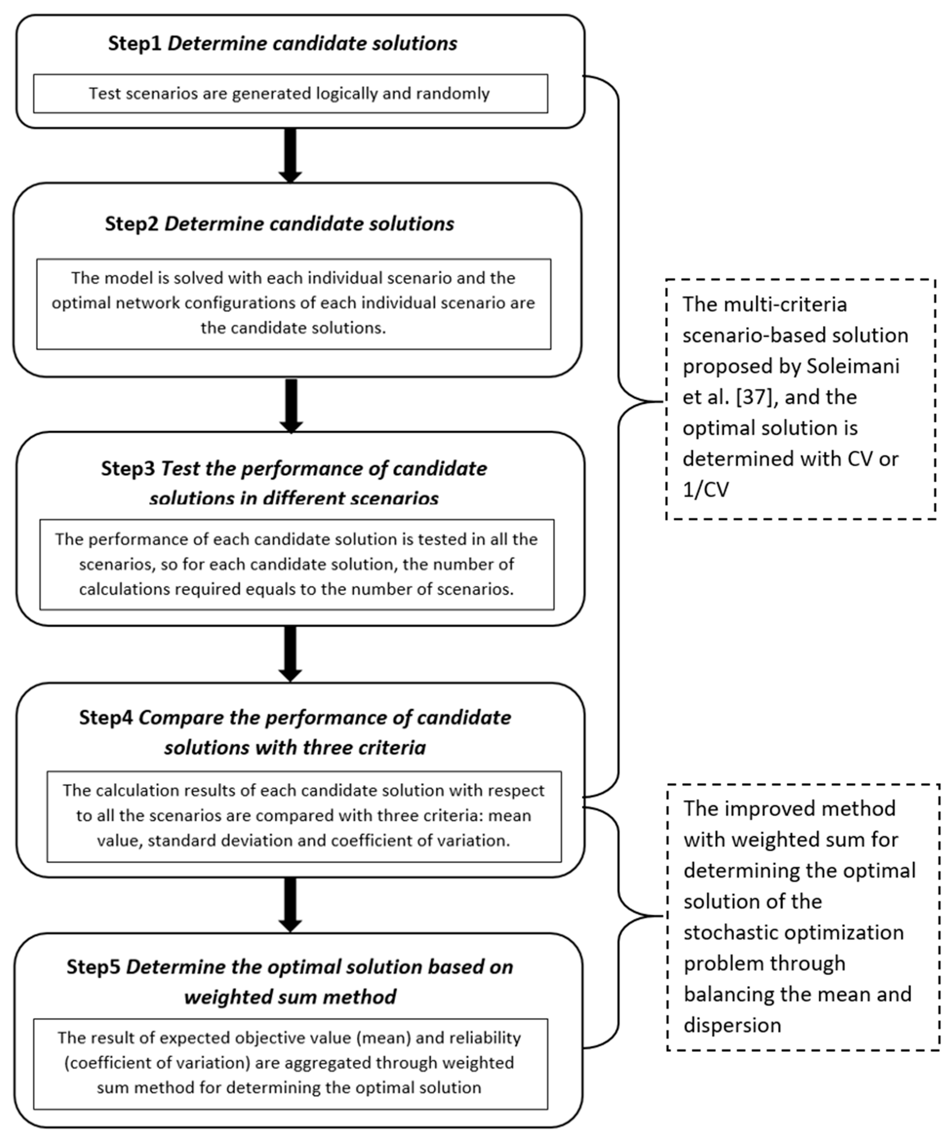Figure 2 presents the solutions procedures of the method, the difference between the improved solution method, and the original solution method is also presented in the figure.

As shown in the figure, the test scenarios with respect to uncertain parameters are first generated logically and randomly, and the introduction of the scenario generation for stochastic programming is provided by Kaut and Wallace [44] and Birge and Louveaux [46]. The candidate solutions are determined based upon the calculation of the optimal solutions of each individual scenario. The objective of a stochastic optimization problem is not to find the optimal solution to a single individual scenario but to determine the solution with the optimal overall performance and reliability through all the possible scenarios. Therefore, each candidate solution is tested with all scenarios, and the performance is evaluated through three criteria: mean value, standard deviation, and coefficient of variation.

Mean value is a very important criterion to evaluate the performance of a series of data (in this case, the optimal costs of reverse logistics network of WEEE with respect to the test scenarios); however, more comprehensive evaluation criteria are needed for reliable and robust decision-making in an uncertain environment. In the multi-criteria scenario-based method, it is important to consider how closely the data approach the mean value, and this requires knowledge about the dispersion of data evaluated by standard deviation. Standard deviation is a well-developed and extensively applied tool used for data analysis in many fields—for example, in the manufacturing industry, the quality of a batch of products can be evaluated by standard deviation; a smaller standard deviation shows a better distribution of the product samples around the required quality level. In the solution method developed by Soleimani et al. [37], the reciprocal of coefficient of variation is applied to connect the mean value and the standard deviation and to determine the optimal solution of the stochastic programming. The basic idea for this solution method is to simultaneously maximize the profit of the supply chain (mean value) and the reliability and robustness of data dispersion or the risk (standard deviation); however, this method has two drawbacks from both mathematical and managerial perspectives.

(1)

From a mathematical perspective, Soleimani et al.’s method is only capable of solving the max-min and min-max problems [37]. For example, it is able to resolve the problem considering the maximum profit and the minimum risk or maximum reliability of the supply chain. However, for the problem formulated in this paper, which is a min-min problem aiming at determining the minimum costs and minimum data dispersion, this solution method is ineffective.

(2)

From a managerial perspective, the managerial meaning of coefficient of variation and its reciprocal are associated with the relative data dispersion compared with the absolute data dispersion determined by standard deviation, but it is not a dedicated tool for determining the optimal solution of a stochastic optimization problem. The theoretical justification of Soleimani et al.’s method [37] is not strong enough to enable comprehensive managerial interpretation. Furthermore, the data dispersion evaluated by standard deviation is significantly affected by the mean value, and this may lead to misinterpretation of the real shape of data dispersion.

In order to solve the aforementioned problems, we improve the multi-criteria scenario-based solution method. First, in our method, coefficient of variation is used to evaluate the reliability and robustness of data dispersion instead of standard deviation, and the managerial meaning of coefficient of variation is introduced. After that, a normalized weighted sum method is applied to aggregate the mean value and coefficient of variation, and the performance of the candidate solutions is evaluated by both expected objective value (mean value) and reliability (coefficient of variation) in order to find the most economic efficient, reliable, and robust solution to the stochastic optimization problem.

Standard deviation is an absolute measurement of data dispersion and is heavily affected by the mean value; if the mean value is different, comparison of standard deviation may not be an appropriate way of evaluating the data dispersion, so another indicator, coefficient of variation, is used to evaluate the reliability of the results. Coefficient of variation, alternatively known as coefficient of dispersion, incorporates both the standard deviation and the mean, and is a unitless indicator applied for measuring the relative dispersion of a series of data [47]:

$$Coefficientofvariation=\frac{Standarddeviation}{Mean}.$$

(30)

Equation (30) illustrates the calculation of coefficient of variation; compared with standard deviation, coefficient of variation can better present the relative data dispersion with respect to different mean values. For example, two types of components (A and B) are inspected through quality control; the mean value of the weight of components A and B are 10 kg and 2 kg, and the standard deviation of the test samples of components A and B are 0.5 kg and 0.3 kg, respectively. Even though the standard deviation of component A is larger than that of component B, the coefficient of variation of component B (0.15) is three times that of component A (0.05), which means the quality of test samples of component A is much better due to the more centered data distribution relative to its mean value.

The optimal solution of the stochastic optimization problem is the one with the lowest expected objective costs (mean value) and the most reliable performance (coefficient of variation), but the best performance of those two objectives is usually not obtained in the same candidate solution. It is important to incorporate both criteria in the design of a reverse logistics system for WEEE. In this paper, we use the weighted sum method to combine the two criteria for selecting the optimal solution of the stochastic optimization problem, and this enables interactions between the subjective input from decision-makers (weight of each criterion) and the objective values of system performance. Furthermore, it is noted that, because of the different measures of units, the two evaluation criteria, mean value and coefficient of variation, are first normalized, as shown in Equation (31):

$$\min OverallPerfomanc{e}_{cand.}=W_M\frac{Mea{n}_{cand.}}{Mea{n}_{min}}+W_C\frac{Coefficientofvariatio{n}_{cand.}}{Coefficientofvariatio{n}_{min}}.$$

(31)

In Equation (31), $Mea{n}_{min}$ and $Coefficientofvariatio{n}_{min}$ are minimum achievable values of the mean and coefficient of variation, and $Mea{n}_{cand.}$ and $Coefficientofvariatio{n}_{cand.}$ are the mean and coefficient of variation of each candidate solution. Through the improvement of the multi-criteria scenario-based solution method, the two drawbacks of the original method can be properly resolved. First, the evaluation of data dispersion by coefficient of variation is a better indicator for the reliability and robustness of reverse logistics system design of WEEE compared with standard deviation. Second, from a mathematical perspective, the introduction of normalized weighted sum method enables the multi-criteria scenario-based solution method to resolve not only max-min and min-max but also min-min and max-max stochastic optimization problems. Third, the improved solution method provides a more reasonable aggregation of the expected optimal value and the reliability, which enables better interpretation of the result.

4. Numerical Experiment

In order to illustrate the applicability of the proposed stochastic optimization programming and the improved solution method in the design and planning of a reverse logistics system for WEEE, a numerical experiment is performed in this section. The numerical experiment includes 10 local collection sites, 5 potential locations for regional collection centers, 5 potential locations for recycling plants, 1 hazardous waste management system, 2 disposal sites, 3 product markets, and 3 material markets. The relevant parameters used in the numerical experiment are randomly generated in a uniformly distributed interval, as shown in

Table 1. Parameter generation in the numerical experiment.

Parameters	Interval
$F{x}_r$	Unif. (4, 5); million USD
$F{x}_p$	Unif. (5, 6); million USD
$Em{s}_r$	Unif. (200, 300); g/ton-capacity
$Em{s}_p$	Unif. (200, 300); g/ton-capacity
$C{p}_d$	Unif. (100, 150); USD
$C{p}_h$	Unif. (500, 600); USD
$d{s}_{cr}$	Unif. (20, 30); km
$d{s}_{rp}$	Unif. (20, 50); km
$d{s}_{rd}$	Unif. (20, 50); km
$d{s}_{rh}$	Unif. (20, 50); km
$d{s}_{pf}$	Unif. (30, 60); km
$d{s}_{pm}$	Unif. (30, 60); km
$d{s}_{pd}$	Unif. (20, 50); km
$C{p}_{rl}$	Unif. (100, 200); USD
$C{p}_{pl}$	Unif. (100, 200); USD
$Ct{r}_{lcr}$/$d{s}_{cr}$	Unif. (1, 2); USD/ton/km
$Ct{r}_{lrp}$/$d{s}_{rp}$	Unif. (1, 2); USD/ton/km
$Ct{r}_{lrd}$/$d{s}_{rd}$	Unif. (4, 5); USD/ton/km
$Ct{r}_{lrh}$/$d{s}_{rh}$	Unif. (2, 3); USD/ton/km
$Ct{r}_{lpf}$/$d{s}_{pf}$	Unif. (1, 2); USD/ton/km
$Ct{r}_{lpm}$/$d{s}_{pm}$	Unif. (1, 2); USD/ton/km
$Ct{r}_{lpd}$/$d{s}_{pd}$	Unif. (2, 3); USD/ton/km
$Em{s}_{lcr}$/$d{s}_{cr}$	Unif. (100, 200); g/ton/km
$Em{s}_{lrp}$/$d{s}_{rp}$	Unif. (100, 200); g/ton/km
$Em{s}_{lrd}$/$d{s}_{rd}$	Unif. (100, 200); g/ton/km
$Em{s}_{lrh}$/$d{s}_{rh}$	Unif. (100, 200); g/ton/km
$Em{s}_{lpf}$/$d{s}_{pf}$	Unif. (100, 200); g/ton/km
$Em{s}_{lpm}$/$d{s}_{pm}$	Unif. (100, 200); g/ton/km
$Em{s}_{lpd}$/$d{s}_{pd}$	Unif. (100, 200); g/ton/km

.

In the numerical experiment, the collected WEEE is categorized into three types: Type-A, Type-B, and Type-C.

Table 2. Parameter generation with respect to different types of WEEE.

Parameters	Interval
	Type A	Type B	Type C
$Co{l}_{lc}^s$	Unif. (500, 600); ton	Unif. (1000, 2000); ton	Unif. (1000, 2000); ton
$PC{p}_{fl}^s$	Unif. (200, 300); USD/ton	Unif. (150, 250); USD/ton	Unif. (150, 250); USD/ton
$PC{m}_{ml}^s$	Unif. (100, 150); USD/ton	Unif. (100, 200); USD/ton	Unif. (100, 200); USD/ton
$Capacit{y}_{rl}$	4000; ton	8000; ton	10,000; ton
$Capacit{y}_{pl}$	3000; ton	5000; ton	8000; ton
${\phi }_{lp}$	50%	60%	60%
${\phi }_{ld}$	20%	20%	30%
${\phi }_{lh}$	30%	20%	10%
${\vartheta }_{lf}$	30%	30%	40%
${\vartheta }_{lm}$	30%	40%	50%
${\vartheta }_{ld}$	40%	30%	10%

illustrates the unit pre-processing costs, unit recycling costs, conversion rate, and capacity at the respective facilities of each type of WEEE. In addition, the unit cost for buying the carbon credits of excessive carbon emissions is 0.000025 USD/g, and the carbon emissions cap for the reverse logistics system for WEEE is 5,000,000 g. It is noteworthy that the units used in the numerical experiment aim mainly at giving readers a better understanding of the applicability of the model, and different measures of units may be applied in the design and planning of the reverse logistics system for WEEE with specific requirements.

In the stochastic optimization model for the design of reverse logistics system for WEEE, the amount of WEEE collected at local collection sites, the price of recycled products, and the price of recycled materials are considered to be uncertain parameters, so several scenarios are generated logically with respect to those uncertain parameters. The basic scenario s0 is the deterministic one with the mean values of the uncertain parameters ($Co{l}_{ac}^{s0}$ = 550 tons, $Co{l}_{bc}^{s0}$ = 1500 tons, $Co{l}_{cc}^{s0}$ = 1500 tons, $PC{p}_{fa}^{s0}$ = 250 USD/ton, $PC{p}_{fb}^{s0}$ = 200 USD/ton, $PC{p}_{fc}^{s0}$ = 200 USD/ton, $PC{m}_{ma}^{s0}$ = 125 USD/ton, $PC{m}_{mb}^{s0}$ = 150 USD/ton, and $PC{m}_{mc}^{s0}$ = 150 USD/ton). For creating the test scenarios, we randomly generated two scenarios for the amount of WEEE collected at local collection sites, two scenarios for the price of recycled products, and two scenarios for the price of recycled materials based upon the uniformly distributed intervals. In total, eight test scenarios (s1, s2, s3, s4, s5, s6, s7, and s8) are generated through the combination of the possibilities of different uncertain parameters.

In addition to the basic and test scenarios, we also generated two benchmarking scenarios: the best-case scenario and the worst-case scenario. In the best-case scenario, the amount of WEEE collected at local collection sites reaches its lower limit while the prices for both recycled products and materials achieve their upper limits ($Co{l}_{ac}^{s9}$ = 500 tons, $Co{l}_{bc}^{s9}$ = 1000 tons, $Co{l}_{cc}^{s9}$ = 1000 tons, $PC{p}_{fa}^{s9}$ = 300 USD/ton, $PC{p}_{fb}^{s9}$ = 250 USD/ton, $PC{p}_{fc}^{s9}$ = 250 USD/ton, $PC{m}_{ma}^{s9}$ = 150 USD/ton, $PC{m}_{mb}^{s9}$ = 200 USD/ton and $PC{m}_{mc}^{s9}$ = 200 USD/ton); this means the reverse logistics system deals with the minimum amount of WEEE with the highest selling price from the recycled products and materials. In the worst-case scenario, the setting of uncertain parameters is an opposite manner ($Co{l}_{ac}^{s10}$ = 600 tons, $Co{l}_{bc}^{s10}$ = 2000 tons, $Co{l}_{cc}^{s10}$ = 2000 tons, $PC{p}_{fa}^{s10}$ = 200 USD/ton, $PC{p}_{fb}^{s10}$ = 150 USD/ton, $PC{p}_{fc}^{s10}$ = 150 USD/ton, $PC{m}_{ma}^{s10}$ = 100 USD/ton, $PC{m}_{mb}^{s10}$ = 100 USD/ton and $PC{m}_{mc}^{s10}$ = 100 USD/ton).

The stochastic programming model is coded in Lingo 11.0 optimization package and the computation of all scenarios is performed on a personal laptop with Intel Core2 duo 2.52 GHz CPU and 4 GB RAM with Windows 7 operating system. At first, the optimal solutions of each individual scenario are calculated as the candidate solutions of the stochastic optimization problem. The problem of each scenario includes 632 decision variables, of which 10 are integers, and all the scenarios can be resolved within 30 s.

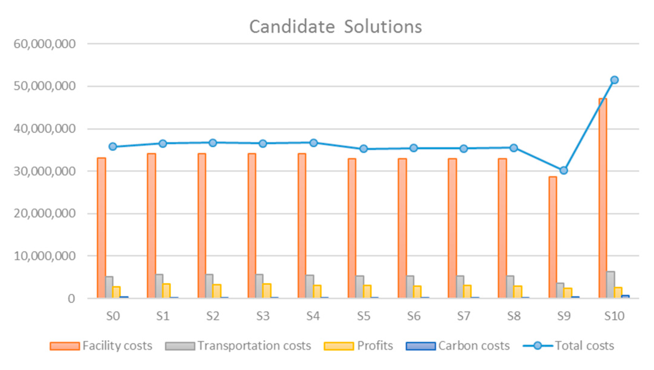
Figure 3 shows the optimal solutions of each individual scenario. As illustrated in the figure, the range of the solution area is 21,411,780 USD (71%), defined by the best-case scenario s9 and the worst case scenario s10. However, when the extreme conditions s9 and s10 are not taken into account, the range of the optimal solutions of the test scenarios (s0–s8) is significantly reduced to 1,429,750 USD (4%). In this case, the mean value is 35,996,637 USD, which leads to a relatively fair distribution of the optimal solutions: s1, s2, s3, and s4 have better performance, while s0, s5, s6, s7, and s8 are slightly below the mean value.

As many have argued (e.g., [48,49]), with the increase of the number of scenarios generated in a stochastic optimization problem, the improvement in the benefits and robustness of the optimal result is relatively limited, but the computational time needed will be drastically increased. Based upon the aforementioned discussion, even though the number of test scenarios generated in the numerical experiment is not very large, they can still represent the solution interval in an effective and efficient manner. In addition, it is observed that, with respect to the test parameters, the facility costs take the most significant share in the overall system costs, and the transportation costs and profits obtained from selling the recycled products and materials are the second and third largest contributor, respectively. However, the contribution of carbon costs is relatively insignificant compared with other types of costs in this example.

The candidate solutions represent the best performance that can be achieved in each individual scenario, but our objective is to find the optimal and most reliable and robust solution through all the possible scenarios. Therefore, the performance of each candidate solution is tested through all the test scenarios; in this example, each candidate solution is calculated 11 times for scenarios s0–s10, so in total 121 calculations are performed in this step. The result is presented in Appendix A (

Table A1. Scenario-based overall system costs of the reverse logistics system for WEEE.

	Sol. s0	Sol. s1	Sol. s2	Sol. s3	Sol. s4	Sol. s5	Sol. s6	Sol. s7	Sol. s8	Sol. s9	Sol. s10
s0	35,801,630	35,952,130	35,801,630	35,801,630	35,801,630	35,801,630	35,801,630	35,875,160	35,801,630	35,801,630	35,801,630
s1	36,718,370	36,548,660	36,718,370	36,718,370	36,718,370	36,718,370	36,718,370	36,746,110	36,718,370	36,718,370	36,718,370
s2	36,893,640	37,110,980	36,726,620	36,893,640	36,893,640	36,893,640	36,893,640	36,921,500	36,893,640	36,893,640	36,893,640
s3	36,727,900	36,783,460	36,727,900	36,558,310	36,727,900	36,727,900	36,727,900	36,755,780	36,727,900	36,727,900	36,727,900
s4	36,908,510	37,181,410	36,908,510	36,908,510	36,736,270	36,908,510	36,908,510	36,936,390	36,908,510	36,908,510	36,908,510
s5	35,472,470	35,472,470	35,472,470	35,472,470	35,472,470	35,306,520	35,472,470	35,472,470	35,472,470	35,472,470	35,472,470
s6	35,633,550	35,825,670	35,633,550	35,633,550	35,633,550	35,633,550	35,470,410	35,633,550	35,633,550	35,633,550	35,633,550
s7	35,494,550	35,519,400	35,494,550	35,494,550	35,494,550	35,494,550	35,494,550	35,328,710	35,494,550	35,494,550	35,494,550
s8	35,655,000	35,871,970	35,655,000	35,655,000	35,655,000	35,655,000	35,655,000	35,655,640	35,492,600	35,655,000	35,655,000
s9	30,292,120	31,104,970	30,292,120	30,292,120	30,292,120	30,292,120	30,292,120	30,607,740	30,292,120	30,136,120	30,292,120
s10	51,547,900	50,812,200	51,547,900	51,547,900	51,547,900	51,547,900	51,547,900	51,573,440	51,547,900	51,547,900	51,547,900
MV 1	37,013,240	37,107,575	36,998,056	36,997,823	36,997,582	36,998,154	36,998,409	37,046,045	36,998,476	36,999,058	37,013,240
SD 2	5,162,559.3	4,837,063.5	5,163,191.8	5,163,749.7	5,163,169.9	5,167,752	5,167,151.5	5,132,479.4	5,167,062.2	5,183,042.5	5,162,559.3
CV 3	0.1394787	0.1303524	0.139553	0.139569	0.1395542	0.1396759	0.1396587	0.1385432	0.139656	0.1400858	0.1394787

¹ MV: Mean value. ² SD: Standard deviation. ³ CV: Coefficient of variance (CV = SD/MV).

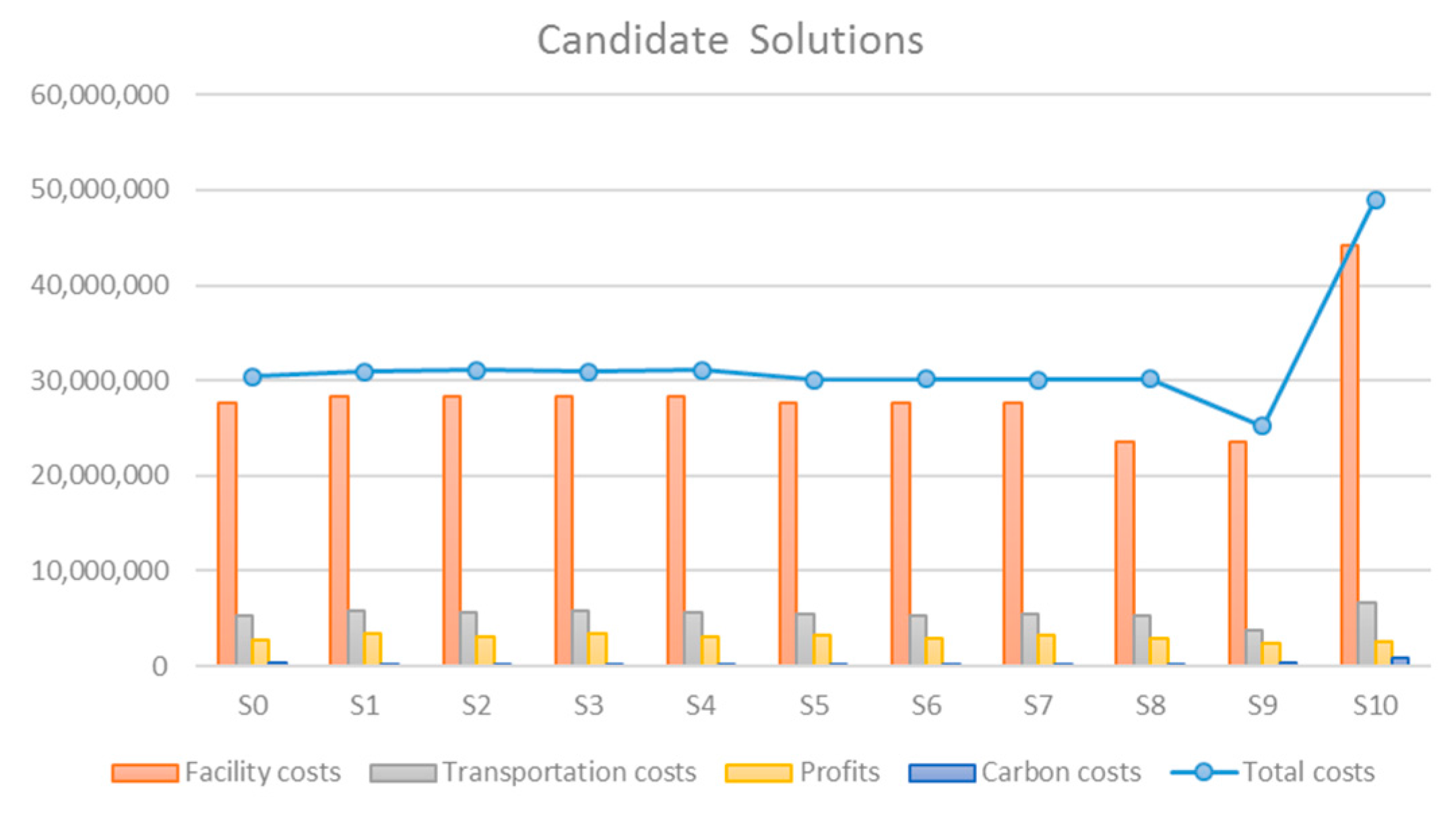
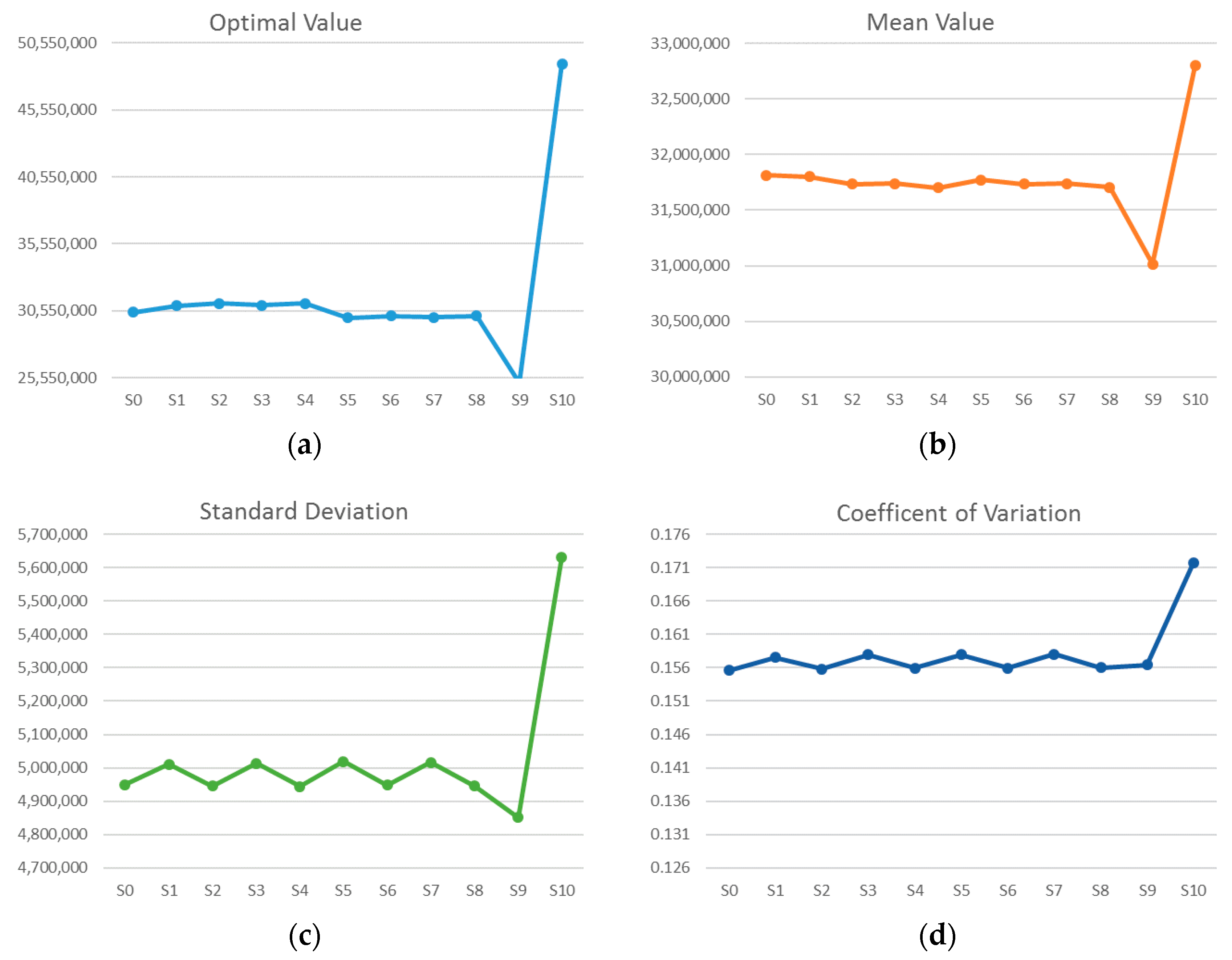
), and Figure 4 illustrates the comparison of the performance of each candidate solution through four criteria: optimal costs, mean costs, standard deviation, and coefficient of variation. Based on the computational results of the example, some managerial implications are discussed as follows.

(1)

As shown in Figure 4a, the best solution of individual optimal costs is achieved in scenario s5 with the lowest system costs of 35,306,520 USD. The optimal cost of the deterministic scenario s0 is the median of the problem, and the optimal costs of scenarios s1, s2, s3, s4, and s10 are higher than the median value, while scenarios s5, s6, s7, s8, and s9 have a better performance in their individual optimal costs.

(2)

As shown in Figure 4b, when the candidate solutions are evaluated through all the test scenarios, the best solution of the mean costs is 36,997,582 USD, achieved in scenario s4, and the worst solution is found for scenario s1, with 37,107,575 USD. It is noteworthy that, in terms of the mean costs, the performance of scenarios s2, s3, s4, s6, s8, and s9 is close to the best performance. Furthermore, it is also observed that the change of mean costs is not correlated to the change of optimal individual costs, which means the better optimal individual costs may not lead to a better overall economic performance in most cases.

(3)

As shown in Figure 4c, when the candidate solutions are evaluated by standard deviation, the best solution is obtained via scenario s1, with the lowest standard deviation at 4,837,063.5 USD, which is far better than the other candidate solutions. This illustrates that the result of candidate solution s1 tested with all possible scenarios has a more centered distribution around the mean value.

(4)

As shown in Figure 4d, in terms of the performance of the coefficient of variation, the best solution is obtained in scenario s2, with the lowest value of coefficient of variation at 0.1303524, which is far better than the other candidate solutions. The second best solution in terms of the coefficient of variation is achieved in scenario s7.

(5)

Comparing Figure 4c with Figure 4d, it is observed that the change of the performance of candidate solutions with respect to standard deviation and coefficient of variation is quite similar, and the influence of the mean costs seems insignificant in this example. This result can be explained by the significant difference in the ranges of mean values and standard deviation. The range of the mean value is only 0.3%, which means the difference between the best and the worst solution is not significant. However, the range between the best solution and the worst solution in standard deviation is 7.2%, which is 24 times higher than that of the mean value, so standard deviation has a much more significant influence on coefficient of variation in this example.

(6)

In this example, $Mea{n}_{min}$ is 36,997,582 USD, obtained from candidate solution s4, and $Coefficientofvariatio{n}_{min}$ is 0.1303524, obtained from candidate solution s1. $W_M$ and $W_C$ denote the weight of the mean and coefficient of variation in the evaluation of the overall performance of the reverse logistics system for WEEE, which reflects the relative importance of the expected objective value and reliability in decision-making. In this example, we test the same weights of the mean (0.5) and coefficient of variation (0.5), and the optimal result is 1.001486, achieved at candidate solution s1; the second and third best solutions equal 1.032073 and 1.035218, obtained through candidate solutions s7, s0 and s10 (s0 and s10 have the same value), respectively. When the optimal overall performance is obtained at candidate solution s1, potential locations r1 and r5 are selected for opening WEEE regional collection centers and potential locations p4 and p5 are selected for opening WEEE recycling plants.

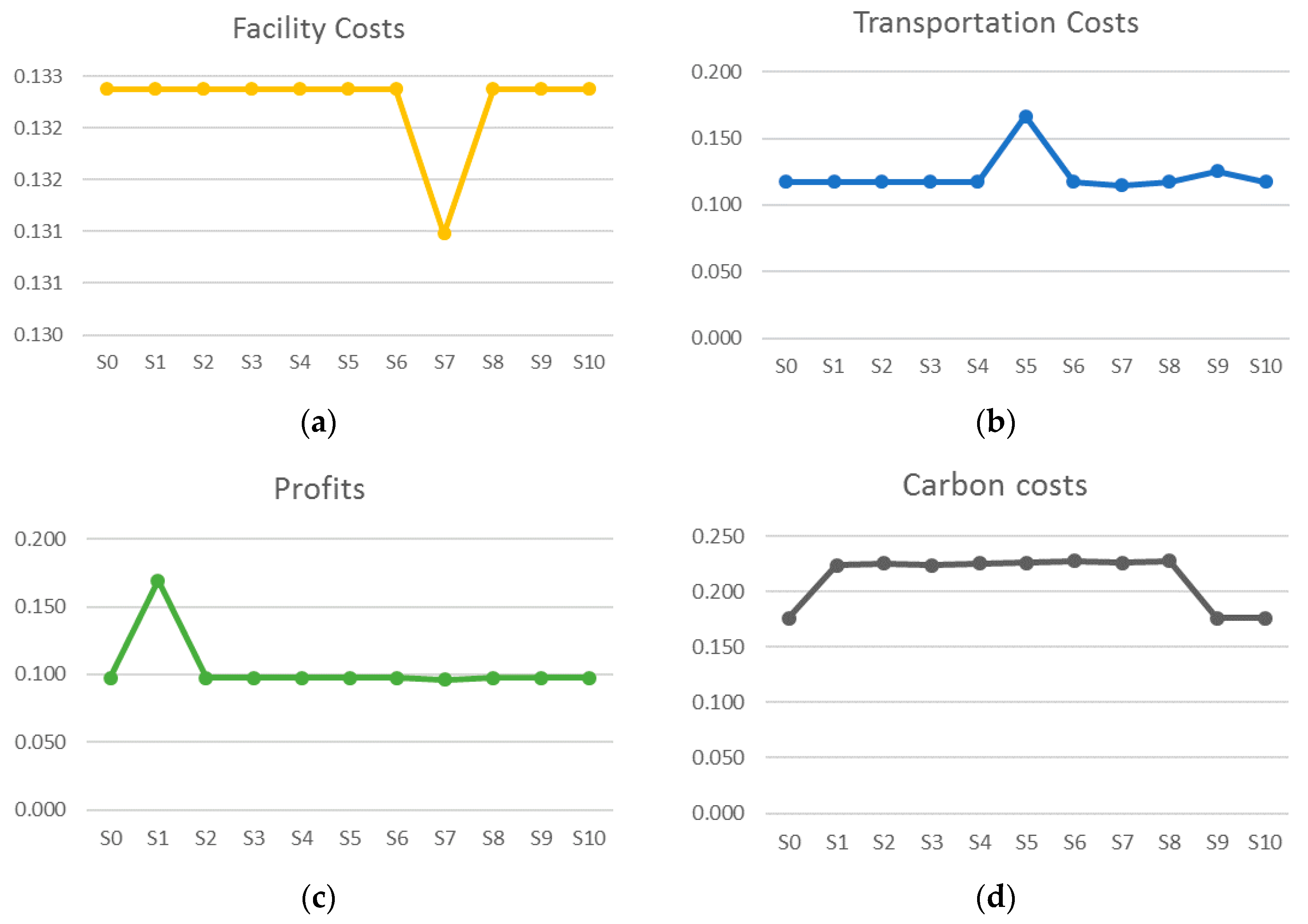
We are also interested in the reliability of different cost components, and Figure 5 shows a comparison of the performance of facility costs, transportation costs, profits obtained from selling the recycled products and materials, and carbon costs in the candidate solutions tested through all possible scenarios. As presented in the figure, we cannot observe a great change in the coefficient of variation in different cost components through most of the candidate solutions. Candidate solution s7 outperforms itself compared with other candidate solutions in the facility costs, which account for the largest share in the overall system costs. Candidate solution s1 has the least reliable performance in the profits gained from the selling of recycled products and materials. With respect to the environmental impacts, candidate solutions s0, s9, and s10 show a more reliable performance than the other candidate solutions. The results reveal that the change in the reliability of individual cost components may not be consistent with that of the overall cost reliability.

In this section, sensitivity analysis with respect to the change of combination of weights is performed, and the result is shown in

Table 3. Sensitivity analysis of the result with respect to the change of weight combination.

Weight Combination		Sol. s0	Sol. s1	Sol. s2	Sol. s3	Sol. s4	Sol. s5	Sol. s6	Sol. s7	Sol. s8	Sol. s9	Sol. s10
${\mathit{W}}_{\mathit{M}}$	${\mathit{W}}_{\mathit{C}}$
0	1	1.070012	1.000000	1.070582	1.070705	1.070592	1.071525	1.071393	1.062836	1.071373	1.074669	1.070012
0.1	0.9	1.063053	1.000297	1.063526	1.063635	1.063532	1.064374	1.064256	1.056683	1.064238	1.067206	1.063053
0.2	0.8	1.056094	1.000595	1.056469	1.056565	1.056473	1.057223	1.057119	1.050531	1.057103	1.059743	1.056094
0.3	0.7	1.049136	1.000892	1.049412	1.049495	1.049414	1.050072	1.049982	1.044378	1.049968	1.052281	1.049136
0.4	0.6	1.042177	1.001189	1.042355	1.042426	1.042355	1.042921	1.042845	1.038225	1.042833	1.044818	1.042177
0.5	0.5	1.035218	1.001486	1.035298	1.035356	1.035296	1.035770	1.035708	1.032073	1.035699	1.037355	1.035218
0.6	0.4	1.028259	1.001784	1.028241	1.028286	1.028237	1.028619	1.028571	1.025920	1.028564	1.029892	1.028259
0.7	0.3	1.021300	1.002081	1.021184	1.021216	1.021177	1.021468	1.021434	1.019768	1.021429	1.022429	1.021300
0.8	0.2	1.014341	1.002378	1.014127	1.014146	1.014118	1.014317	1.014297	1.013615	1.014294	1.014966	1.014341
0.9	0.1	1.007382	1.002676	1.007070	1.007076	1.007059	1.007166	1.007159	1.007462	1.007159	1.007503	1.007382
1	0	1.000423	1.002973	1.000013	1.000007	1.000000	1.000015	1.000022	1.001310	1.000024	1.000040	1.000423

. The weight of expected objective value $W_M$ increases from 0 to 1 by steps of 0.1, and the weight of reliability $W_C$ decreases in the opposite way. As illustrated in the table, candidate solution s1 has the optimal overall performance through most scenarios with different combinations of weights (expect the last one) due to its high reliability (lowest coefficient of variation). It is noteworthy that the optimal solution of this example is similar to the calculation with our solution method and Soleimani et al.’s solution method [37]. However, with the increase in the weight of the mean value, the second and third best solutions may change significantly. For example, when $W_M$ equals 0.9 and $W_C$ equals 0.1, the second best solution is 1.007059, obtained in candidate solution s4, and the third best solution is 1.007070, obtained at candidate solution s2. This illustrates that the subjective weight combination determined by the decision-makers may significantly affect the optimal result of the stochastic optimization problem.

5. Sensitivity Analysis

We are interested in the influence of the change of some key parameters in the design of reverse logistics system for WEEE, and two sensitivity analyses (SA and S-B) are performed in this section. The facility capacity limitation is the bottleneck of the reverse logistics system for WEEE in the previous section. The literature has shown that facility expansion at the same location is much more efficient in dealing with increased customer demand than opening new facilities [50]. Therefore, in the first sensitivity analysis S-A, we increase the facility capacity of different types of WEEE by 100% at regional collection centers and recycling plants, and the fixed facility costs are increased by 40% due to the increase in the resources invested in facility expansion, i.e., equipment, personnel, etc.

The result of sensitivity analysis S-A is illustrated in Appendix B (

Table B1. Scenario-based overall system costs of the reverse logistics system for WEEE in sensitivity analysis (A).

	Sol. s0	Sol. s1	Sol. s2	Sol. s3	Sol. s4	Sol. s5	Sol. s6	Sol. s7	Sol. s8	Sol. s9	Sol. s10
s0	30,433,820	30,710,800	30,451,520	30,593,350	30,334,070	30,710,800	30,451,520	30,593,350	30,334,070	29,651,950	31,215,700
s1	31,251,300	30,937,490	31,134,170	30,789,760	31,176,440	30,747,490	31,134,170	30,789,760	31,176,440	30,416,190	32,086,410
s2	31,408,420	31,530,740	31,091,320	31,573,010	31,294,760	31,530,740	31,252,500	31,573,010	31,294,760	30,573,310	32,243,530
s3	31,586,510	31,183,690	31,570,370	30,959,830	31,511,650	31,183,690	31,570,370	31,124,970	31,511,650	30,751,400	32,421,620
s4	31,394,940	31,618,250	31,340,010	31,559,530	31,113,650	31,618,250	31,340,010	31,559,530	31,281,290	30,559,830	32,230,050
s5	30,670,490	30,210,790	30,537,930	30,247,360	30,574,500	30,049,090	30,537,930	30,247,360	30,574,500	29,898,040	31,442,940
s6	30,478,020	30,585,080	30,329,100	30,621,640	30,365,660	30,585,080	30,171,130	30,621,640	30,365,660	29,705,560	31,250,470
s7	30,649,910	30,293,480	30,620,610	30,226,780	30,553,910	30,293,480	30,620,610	30,065,270	30,553,910	29,877,450	31,422,360
s8	30,416,720	30,644,330	30,376,820	30,577,630	30,310,120	30,644,330	30,376,820	30,577,630	30,187,320	29,626,270	31,207,180
s9	25,749,000	25,939,050	25,768,800	25,849,950	25,679,700	25,939,050	25,768,800	25,849,950	25,679,700	25,212,750	26,285,250
s10	45,929,180	46,175,180	45,874,080	46,115,780	45,814,680	46,175,180	45,874,080	46,115,780	45,814,680	44,901,680	48,997,110
MV 1	31,815,301	31,802,625	31,735,885	31,737,693	31,702,649	31,770,653	31,736,176	31,738,023	31,706,725	31,015,857	32,800,238
SD 2	4,950,109.6	5,010,178.7	4,945,815.7	5,013,603.6	4,944,127.9	5,019,098.1	4,948,722.4	5,016,440	4,946,024	4,851,587.7	5,632,609.1
CV 3	0.155589	0.1575398	0.155843	0.15797	0.1559531	0.1579791	0.1559332	0.1580577	0.1559928	0.1564228	0.1717246

¹ MV: Mean value. ² SD: Standard deviation. ³ CV: Coefficient of variance (CV = SD/MV).

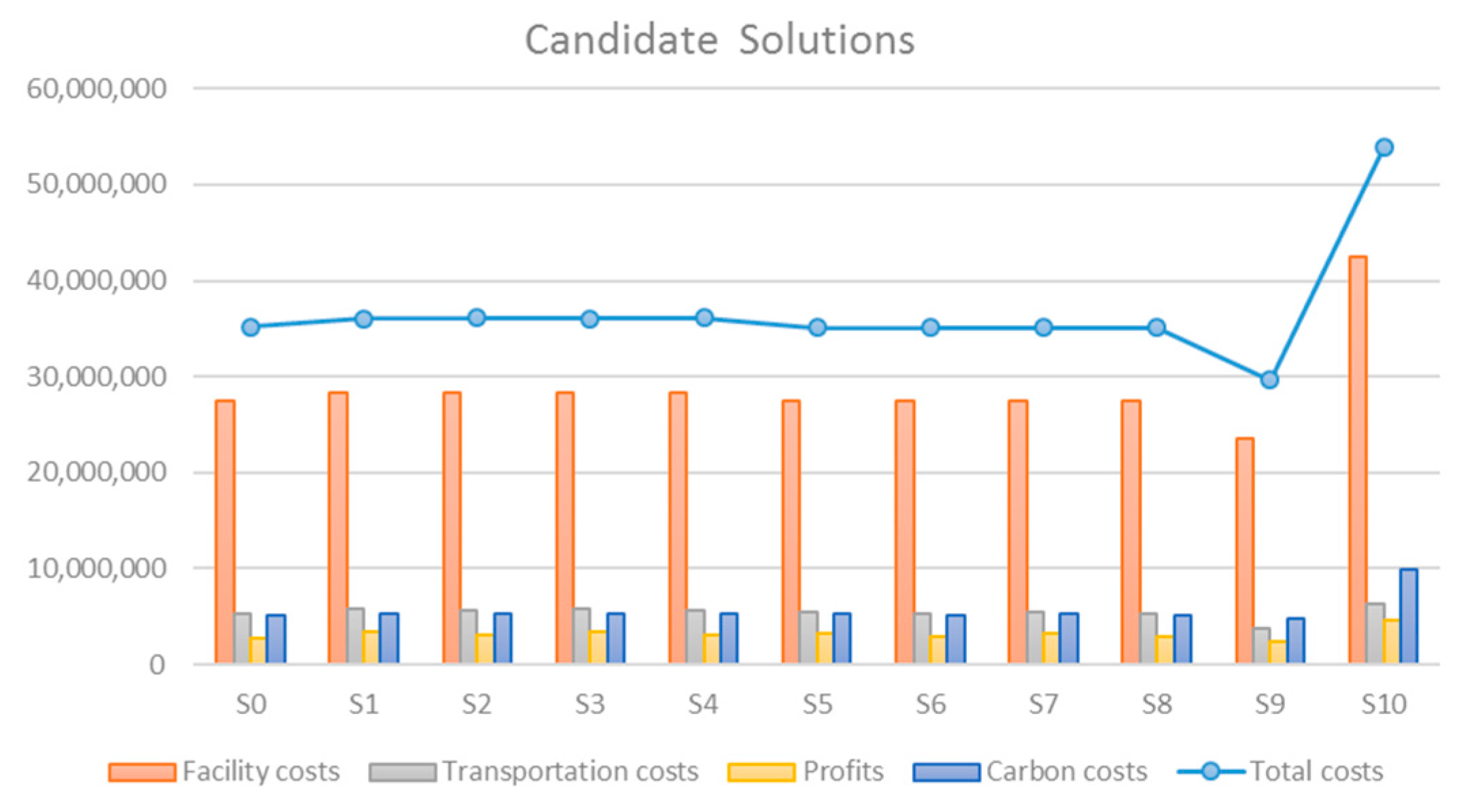
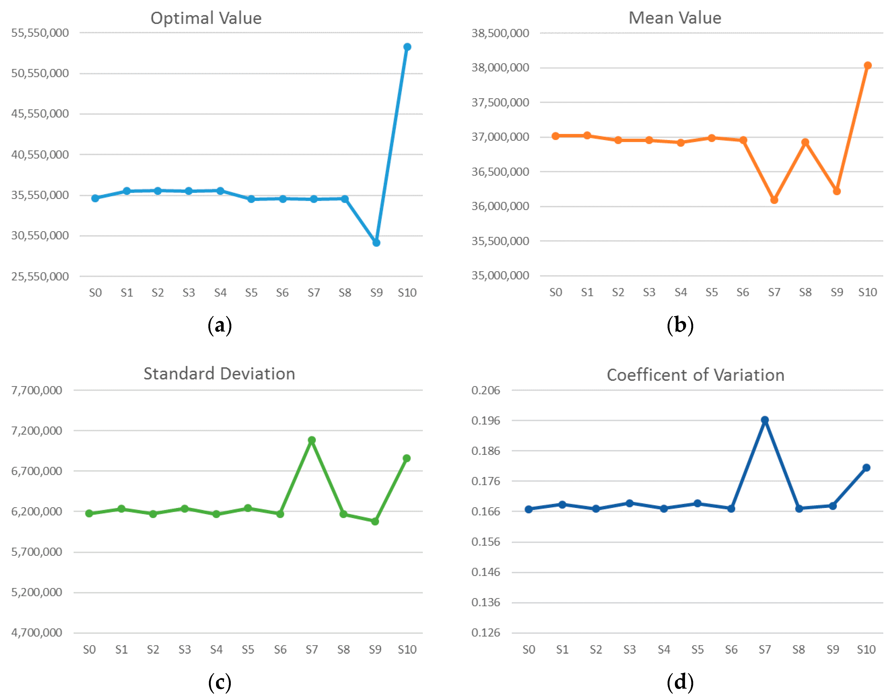
), Figure 6 and Figure 7, and

Table 4. Sensitivity analysis of the results with respect to the change of weight combination (S-A).

Weight Combination		Sol. s0	Sol. s1	Sol. s2	Sol. s3	Sol. s4	Sol. s5	Sol. s6	Sol. s7	Sol. s8	Sol. s9	Sol. s10
${\mathit{W}}_{\mathit{M}}$	${\mathit{W}}_{\mathit{C}}$
0	1	1.000000	1.012538	1.001633	1.015303	1.002341	1.015362	1.002212	1.015867	1.002596	1.005359	1.103707
0.1	0.9	1.002578	1.013821	1.003791	1.016100	1.004321	1.016259	1.004313	1.016609	1.004564	1.004823	1.099090
0.2	0.8	1.005155	1.015104	1.005949	1.016897	1.006301	1.017156	1.006415	1.017351	1.006532	1.004287	1.094472
0.3	0.7	1.007733	1.016387	1.008107	1.017694	1.008281	1.018054	1.008516	1.018092	1.008500	1.003752	1.089854
0.4	0.6	1.010310	1.017670	1.010266	1.018491	1.010262	1.018951	1.010617	1.018834	1.010468	1.003216	1.085237
0.5	0.5	1.012888	1.018952	1.012424	1.019288	1.012242	1.019849	1.012718	1.019576	1.012435	1.002680	1.080619
0.6	0.4	1.015465	1.020235	1.014582	1.020085	1.014222	1.020746	1.014819	1.020317	1.014403	1.002144	1.076002
0.7	0.3	1.018043	1.021518	1.016740	1.020882	1.016202	1.021644	1.016921	1.021059	1.016371	1.001608	1.071384
0.8	0.2	1.020620	1.022801	1.018898	1.021679	1.018183	1.022541	1.019022	1.021800	1.018339	1.001072	1.066766
0.9	0.1	1.023198	1.024084	1.021057	1.022476	1.020163	1.023438	1.021123	1.022542	1.020307	1.000536	1.062149
1	0	1.025775	1.025367	1.023215	1.023273	1.022143	1.024336	1.023224	1.023284	1.022275	1.000000	1.057531

. As illustrated in the figures and tables, the overall system costs are reduced by approximately 15% compared with the result of the previous numerical experiment, the optimal mean value is achieved at candidate solution s0, and the optimal coefficient of variation is obtained at candidate solution s9. When the weights of expected objective value and reliability are identical, the optimal solution is 1.002680, obtained at candidate solution s9, potential location r1 is selected to open the regional collection center, and potential location p5 is selected for the new recycling plant. It is noteworthy that, with the increase in facility capacity, only two new facilities are opened in sensitivity analysis S-A for the treatment of WEEE, and the overall facility costs are significantly reduced due to the decreased number of facilities opened, even though the fixed operating costs of each individual facility increase by 40%. This result has revealed the effectiveness of capacity expansion at existing facilities. Compared with opening new facilities, the possible capacity expansion may drastically reduce the overall system costs due to the cost savings from construction, aggregation of transportation, and economy of scale. This result is valuable for decision-making about reverse logistics system design and planning for treating the increased amount of WEEE, particularly from a long-term perspective.

Compared with other types of costs, the carbon emissions costs are relatively insignificant in the overall system costs of the reverse logistics system for WEEE. We are interested in finding out whether a more stringent environmental policy can play an important role in the design of a reverse logistics system for WEEE. In the second sensitivity analysis S-B, two changes are made to minimize the environmental impacts of the reverse logistics system for WEEE. First, the carbon cap is reduced to 0, which means all the carbon emissions from the reverse logistics system will be charged. In addition, the unit cost for buying carbon credits is increased 10 times, which means much more will be paid for the carbon emissions. Sensitivity analysis S-B is conducted to test the result of the problem in an extreme condition in which environmental sustainability is made one of the first priorities, and it can be used for policy-making and a reconfiguration of the reverse logistics system in the coming years.

The result of the sensitivity analysis S-B is illustrated in Appendix B (

Table B2. Scenario-based overall system costs of the reverse logistics system for WEEE in sensitivity analysis (B).

	Sol. s0	Sol. s1	Sol. s2	Sol. s3	Sol. s4	Sol. s5	Sol. s6	Sol. s7	Sol. s8	Sol. s9	Sol. s10
s0	35,217,930	35,511,820	35,252,540	35,394,370	35,135,090	35,511,820	35,252,540	35,394,370	35,135,090	34,452,970	36,016,720
s1	36,188,520	36,055,660	36,071,390	35,726,980	36,113,660	35,684,710	36,071,390	35,726,980	36,113,660	35,353,410	37,023,630
s2	36,284,990	36,407,310	36,111,890	36,449,570	36,171,330	36,407,310	36,129,070	36,449,570	36,171,330	35,449,880	37,387,200
s3	36,552,090	36,149,270	36,535,950	36,073,380	36,477,230	36,149,270	36,535,950	36,090,550	36,477,230	35,716,980	37,387,200
s4	36,267,670	36,490,970	36,212,730	36,432,250	36,129,610	36,490,970	36,212,730	36,432,250	36,154,010	35,432,560	37,102,780
s5	35,558,890	35,099,190	35,426,330	35,135,750	35,462,890	35,081,860	35,426,330	35,135,750	35,462,890	34,786,430	36,331,340
s6	35,282,160	35,389,220	35,133,240	35,425,790	35,169,800	35,389,220	35,115,900	35,425,790	35,169,800	34,509,710	36,054,620
s7	35,533,790	35,177,360	35,504,490	35,110,650	35,437,790	35,177,360	35,504,490	35,093,320	35,437,790	34,761,330	36,306,240
s8	35,219,260	35,446,870	35,179,360	35,380,170	35,112,660	35,446,870	35,179,360	30,325,590	35,127,370	34,428,810	36,009,720
s9	30,224,640	30,414,690	30,244,440	30,325,590	30,155,340	30,414,690	30,244,440	25,849,950	30,155,340	29,673,020	30,760,890
s10	54,892,650	55,138,650	54,837,550	55,079,250	54,778,150	55,138,650	54,837,550	55,079,250	54,778,150	53,865,150	57,978,850
MV 1	37,020,235	37,025,546	36,955,446	36,957,614	36,922,141	36,990,248	36,955,432	36,091,215	36,925,696	36,220,932	38,032,654
SD 2	6,176,398.2	6,235,000.1	6,171,274.3	6,238,725	6,168,802.5	6,242,297.6	6,171,556.3	7,084,390.6	6,168,063	6,081,694.7	6,865,778.5
CV 3	0.1668384	0.1683972	0.1669923	0.1688076	0.167076	0.1687552	0.1669999	0.1962913	0.1670399	0.1679055	0.1805232

¹ MV: Mean value. ² SD: Standard deviation. ³ CV: Coefficient of variance (CV = SD/MV).

), Figure 8 and Figure 9, and

Table 5. Sensitivity analysis of the result with respect to the change of weight combination (S-B).

Weight Combination		Sol. s0	Sol. s1	Sol. s2	Sol. s3	Sol. s4	Sol. s5	Sol. s6	Sol. s7	Sol. s8	Sol. s9	Sol. s10
${\mathbf{W}}_{\mathbf{M}}$	${\mathbf{W}}_{\mathbf{C}}$
0	1	1.000000	1.009343	1.000922	1.011803	1.001424	1.011489	1.000968	1.176535	1.001207	1.006396	1.082024
0.1	0.9	1.002574	1.010998	1.003224	1.013023	1.003584	1.012831	1.003266	1.158882	1.003399	1.006116	1.079201
0.2	0.8	1.005148	1.012652	1.005527	1.014243	1.005744	1.014173	1.005564	1.141228	1.005590	1.005836	1.076378
0.3	0.7	1.007722	1.014307	1.007829	1.015464	1.007903	1.015515	1.007861	1.123575	1.007782	1.005555	1.073555
0.4	0.6	1.010296	1.015961	1.010132	1.016684	1.010063	1.016857	1.010159	1.105921	1.009973	1.005275	1.070732
0.5	0.5	1.012870	1.017616	1.012434	1.017904	1.012223	1.018199	1.012457	1.088268	1.012164	1.004995	1.067908
0.6	0.4	1.015445	1.019270	1.014736	1.019125	1.014383	1.019542	1.014755	1.070614	1.014356	1.004715	1.065085
0.7	0.3	1.018019	1.020925	1.017039	1.020345	1.016543	1.020884	1.017052	1.052961	1.016547	1.004435	1.062262
0.8	0.2	1.020593	1.022579	1.019341	1.021565	1.018703	1.022226	1.019350	1.035307	1.018739	1.004154	1.059439
0.9	0.1	1.023167	1.024234	1.021643	1.022785	1.020863	1.023568	1.021648	1.017654	1.020930	1.003874	1.056616
1	0	1.025741	1.025888	1.023946	1.024006	1.023023	1.024910	1.023945	1.000000	1.023121	1.003594	1.053793

. As shown in the figures and tables, the stringent environmental requirements lead to much higher overall costs for the reverse logistics system for WEEE due to the great increase in carbon emissions costs. The optimal mean value and coefficient of variation are obtained at candidate solutions s0 and s9, respectively. When $W_M$ equals 0.5 and $W_C$ equals 0.5, the optimal solution is 1.004995, achieved at candidate solution s9, and potential locations r1 and p5 are selected for new facilities. The facility selection is the same as that in sensitivity analysis S-A, which shows the consistency between economic efficiency and environmental impact. In other words, an optimal and reliable configuration of a reverse logistics system for WEEE through location optimization and transportation aggregation may bring both economic and environmental benefits.

The results of the illustrative example and sensitivity analyses clearly show the difference in the computation of the optimal solution of the stochastic optimization problem between the improved multi-criteria scenario-based solution method and the original solution method developed by Soleimani et al. [37]. In some cases, similar results may be obtained with both methods, but different results are achieved in most cases. This reveals that the multi-criteria scenario-based solution method developed in this paper has a better applicability for stochastic optimization problems, especially for min-min or max-max problems. Furthermore, our solution method provides more comprehensive managerial interpretation for the evaluation of the reliability and robustness of data dispersion.

6. Conclusions

Today, the increased public concern about sustainable development and more stringent environmental regulations have become important driving forces for value recovery from end-of-life and end-of use products through reverse logistics. This paper presents a novel stochastic mixed integer programming model for the design of a generic multi-source, multi-echelon, and capacitated reverse logistics system for WEEE in an economic efficient and environmental friendly manner. The model aims at minimizing the overall costs of the reverse logistics system for WEEE through location optimization and transportation planning, and the amount of WEEE generated at local collection sites, price of recycled products, and recycled materials are considered as uncertain parameters. Furthermore, the model takes into account the environmental impacts of reverse logistics; in this paper, the environmental impacts are evaluated in terms of carbon emissions costs. The proposed stochastic optimization model is resolved with an improved multi-criteria scenario-based solution method and coded in Lingo 11.0 optimization solver, and a numerical example and sensitivity analyses are conducted in order to illustrate the application of the model and provide managerial insights for decision-making. The main contributions of the paper are summarized as follows:

(1)

The paper provides a novel stochastic optimization model for the design of a generic reverse logistics system for WEEE. Reverse logistics is characterized as having a high level of uncertainty, so the modelling and formulation of some uncertain parameters are of significant importance.

(2)

Compared with previous mathematical models, the model proposed in this paper considers the environmental impacts of the reverse logistics system for WEEE, and the minimization of carbon emissions is also a very important consideration of the model.

(3)

The model is resolved with the multi-criteria scenario-based solution method in order to find the most economically efficient and reliable solution to the stochastic optimization problem. The expected objective value and reliability are evaluated by the mean and coefficient of variation, and normalized weighted sum formulation is applied to combine the two evaluation criteria. The solution method enables interactions between the subjective evaluation from the decision makers and the objective system values, so the result achieved is more reliable and robust. In addition, our improved solution method also resolves the deficiencies of the original solution method, and is capable of solving min-min and max-max optimization problems. In addition, the managerial meaning of the solution method is explicitly explained in this paper.

(4)

The numerical experiment and sensitivity analyses provide valuable managerial insights into the design of a reverse logistics system for WEEE. For example, capacity expansion at existing facilities may be a more economically efficient way for dealing with an increased amount of WEEE, and both economic and environmental performance may be improved simultaneously with location optimization and transportation aggregation. In addition, the managerial insight from the system design and planning of a reverse logistics network of WEEE may also provide valuable information for the government in determining a subsidy scheme for companies performing WEEE treatment.

For further development of this research, four suggestions are proposed. First, for large sized stochastic mixed integer programming, some advanced solution methods, i.e., meta-heuristic [51,52], should be developed and applied to the design of a reverse logistics system for WEEE in order to improve the computational efficiency and effectiveness. Second, the model may be further developed into a multi-objective programming model in order to take into account more comprehensive considerations in the design of the reverse logistics system for WEEE, i.e., risk [53,54,55,56,57], saving of resources [42], etc. Third, the model is developed primarily for addressing the general characteristics of the reverse logistics system for WEEE from a strategic perspective; however, some specific technologies are used in the sorting and recycling processes of WEEE, so future research may focus on the economic efficiency and environmental impacts of those specific technologies for the processing and treatment of WEEE. Fourth, the application and validation of the proposed stochastic optimization model with a real-world case study of the design and planning of the reverse logistics system for WEEE will be expected in the future.