Detecting the Spatially Non-Stationary Relationships between Housing Price and Its Determinants in China: Guide for Housing Market Sustainability


Abstract
:1. Introduction
2. Literature Review
3. Variables and Data Processing
3.1. Variables
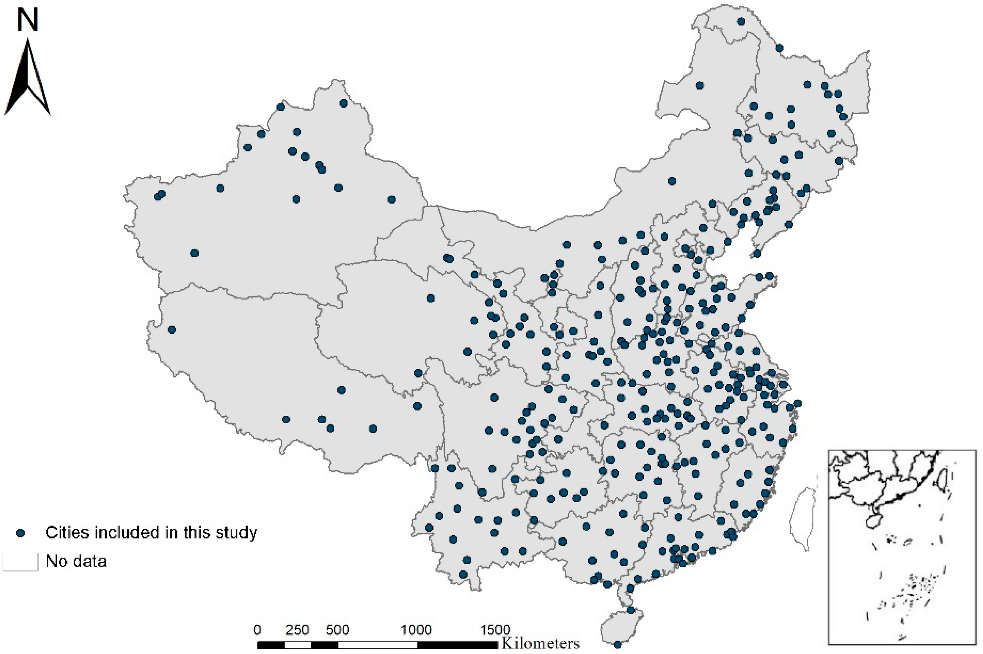
3.2. Study Area
3.3. Data Sources and Processing
4. Methods
4.1. Model Fitting
4.2. Model Evaluation
4.3. Geographically Weighted Regression
5. Results and Discussion
5.1. Model Performance and Estimates
5.2. Discussion of Estimated Coefficients
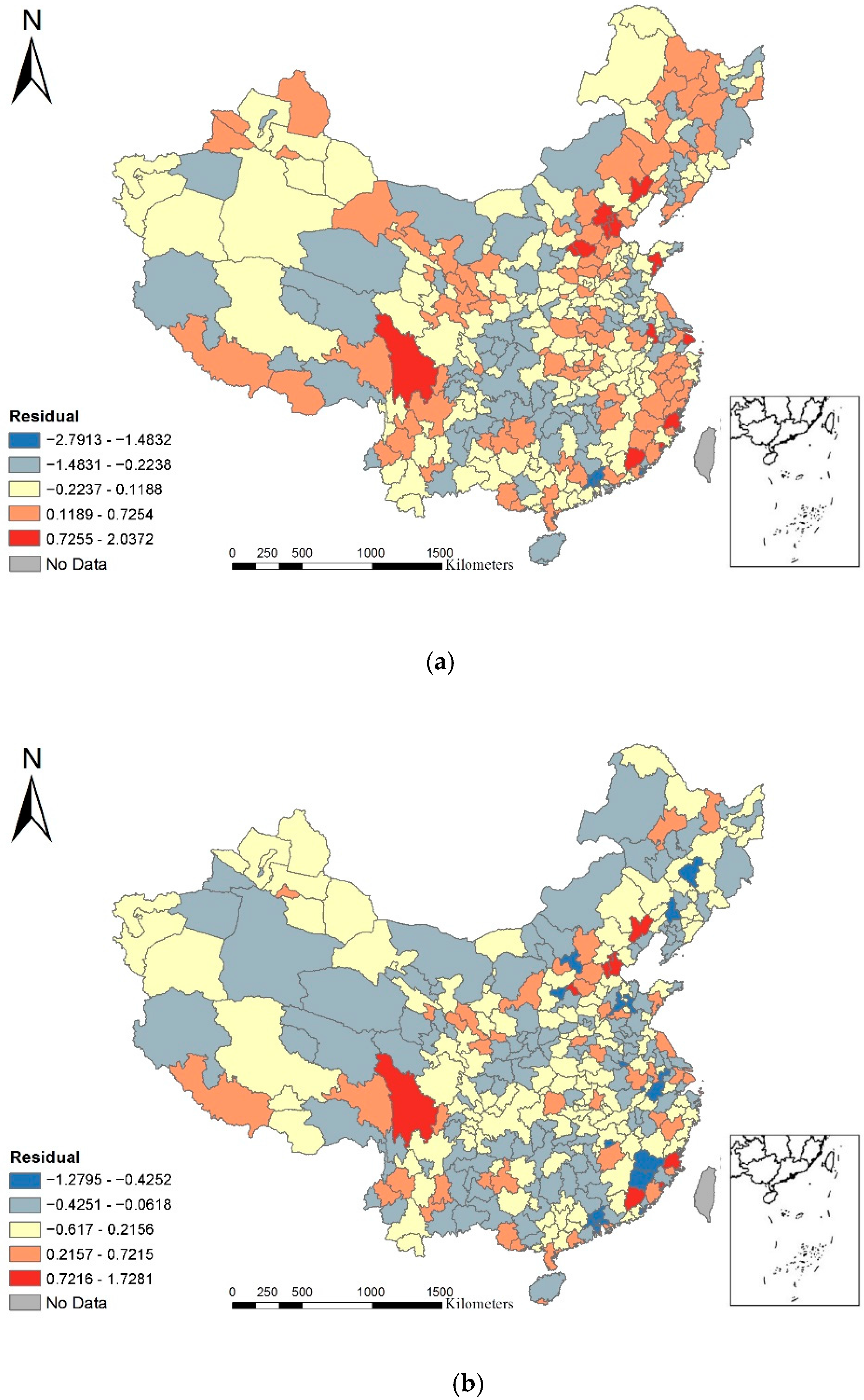
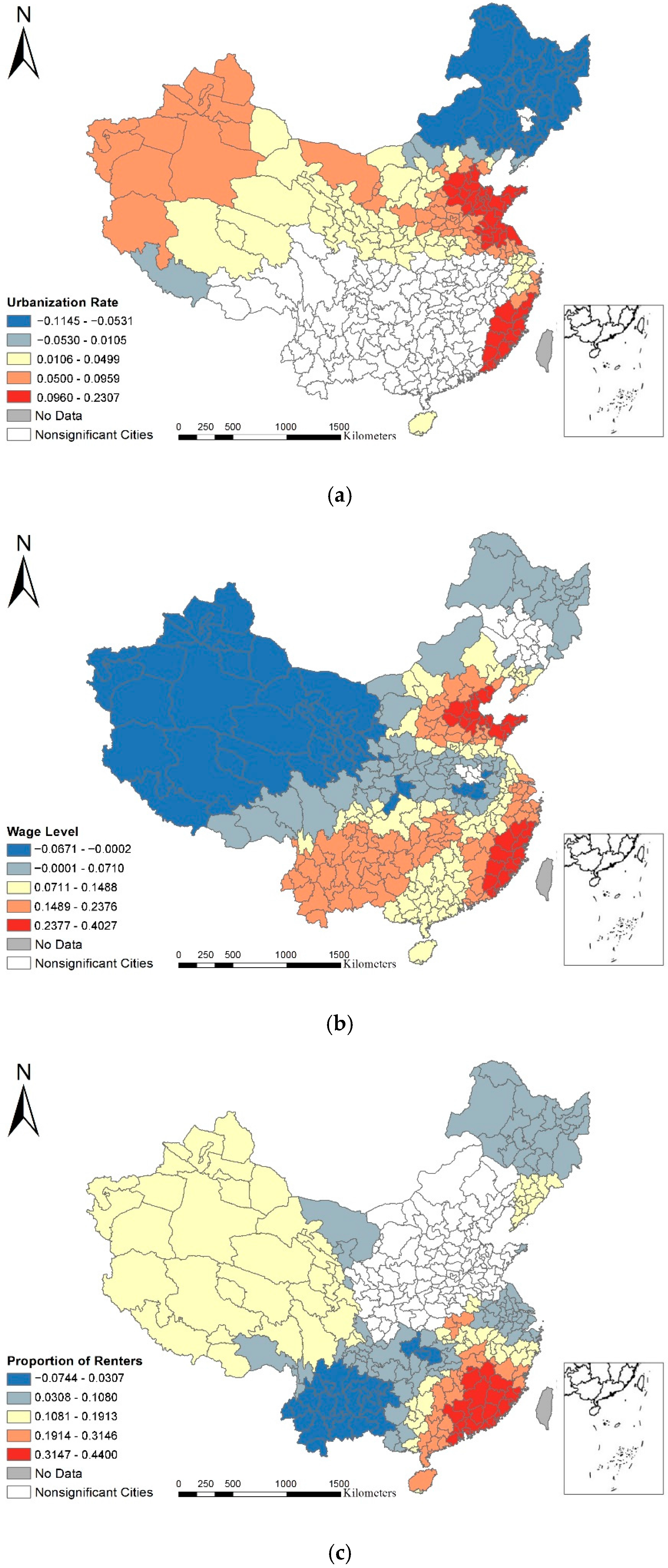
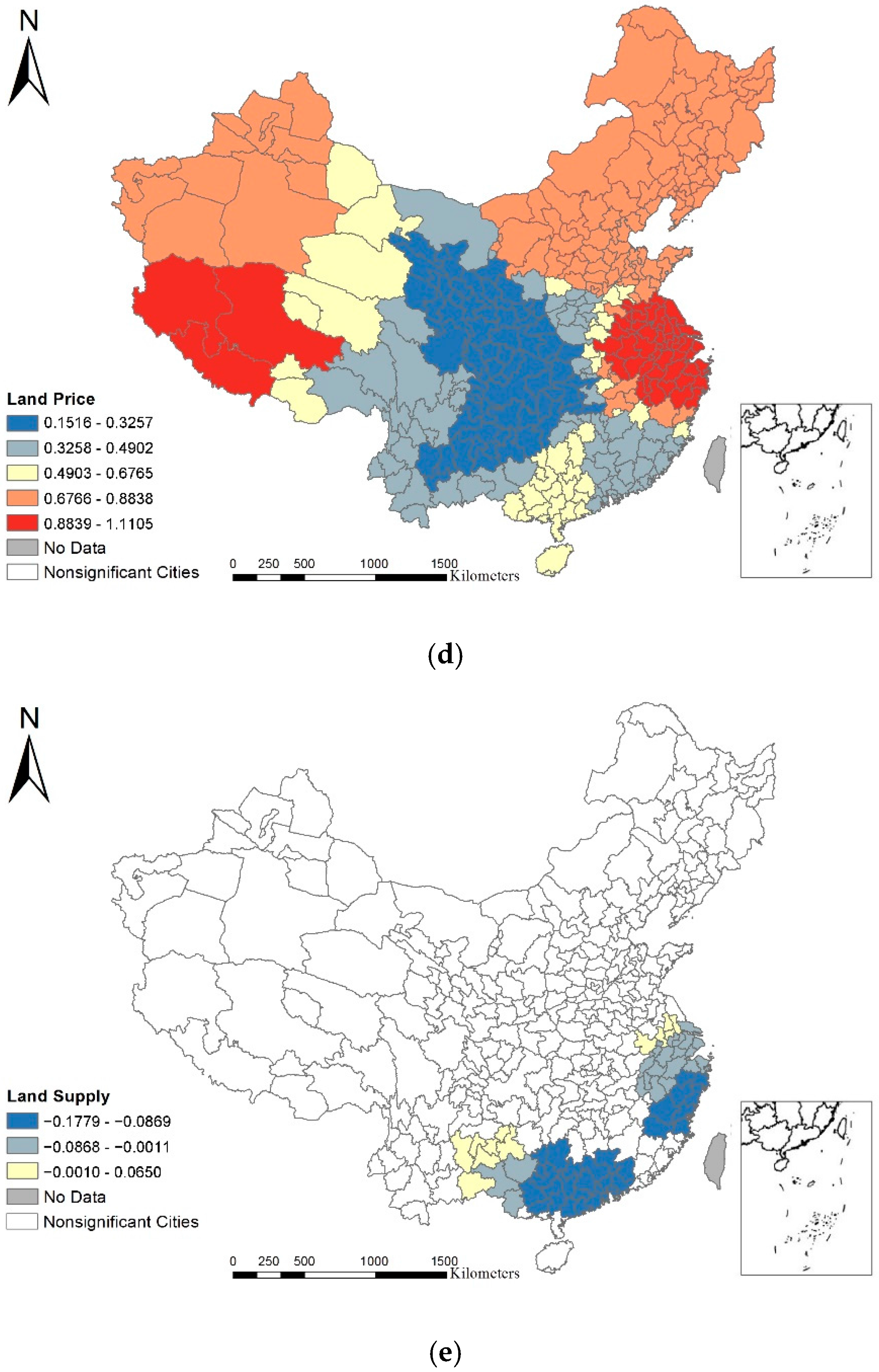
5.3. Spatial Pattern
6. Conclusions and Policy Implications
6.1. Conclusions
6.2. Policy Implications for Sustainability in the Housing Market
“The first step is to develop housing rental enterprises by supporting built or new housing to be used as rentals. Second, the government should subsidize households income limits by providing public housing. Third is to improve tax incentives and encourage financial institutions to increase support and the supply of rental housing land. Fourth, strengthening supervision and standardizing intermediary services is also an important means to stabilize the tenancy relationship and protect the legitimate rights and interests of the lessee.”
Acknowledgments
Author Contributions
Conflicts of Interest
References
- Shih, Y.; Li, H.; Qin, B. Housing price bubbles and inter-provincial spillover: Evidence from China. Habitat Int. 2014, 43, 142–151. [Google Scholar] [CrossRef]
- Li, C.; Gibson, J. Spatial price differences and inequality in China: Housing market evidence. Work. Pap. Econ. 2013, 6, 13. [Google Scholar]
- Wang, Y.P. Urban housing reform and finance in China a case study of Beijing. Urban Aff. Rev. 2001, 36, 620–645. [Google Scholar] [CrossRef]
- Chen, J.; Guo, F.; Wu, Y. One decade of urban housing reform in China: Urban housing price dynamics and the role of migration and urbanization, 1995–2005. Habitat Int. 2011, 35, 1–8. [Google Scholar] [CrossRef]
- Shi, W.; Chen, J.; Wang, H. Affordable housing policy in China: New developments and new challenges. Habitat Int. 2016, 54, 224–233. [Google Scholar] [CrossRef]
- Zhang, L.; Hui, E.C.; Wen, H. Housing price–volume dynamics under the regulation policy: Difference between Chinese coastal and inland cities. Habitat Int. 2015, 47, 29–40. [Google Scholar] [CrossRef]
- Manning, C.A. Intercity differences in home price appreciation. J. Real Estate Res. 1986, 1, 45–56. [Google Scholar]
- Wang, Z.; Zhang, Q. Fundamental factors in the housing markets of China. J. Hous. Econ. 2014, 25, 53–61. [Google Scholar] [CrossRef]
- Wang, Y.; Wang, D.; Wei, Y. Spatial differentiation patterns of housing price and housing price-to-income ratio in China’s cities. In Proceedings of the 2013 21st International Conference on Geoinformatics, Kaifeng, China, 20–22 June 2013. [Google Scholar]
- Wang, Y.; Wang, S.; Li, G.; Zhang, H.; Jin, L.; Su, Y.; Wu, K. Identifying the determinants of housing prices in China using spatial regression and the geographical detector technique. Appl. Geogr. 2017, 79, 26–36. [Google Scholar] [CrossRef]
- Gardiner, B.; Martin, R.; Sunley, P.; Tyler, P. Spatially unbalanced growth in the British economy. J. Econ. Geogr. 2013. [Google Scholar] [CrossRef]
- Rothenberg, J. The Maze of Urban Housing Markets: Theory, Evidence, and Policy; University of Chicago Press: Chicago, IL, USA, 1991. [Google Scholar]
- Anselin, L. Lagrange multiplier test diagnostics for spatial dependence and spatial heterogeneity. Geogr. Anal. 1988, 20, 1–17. [Google Scholar] [CrossRef]
- Leung, Y.; Mei, C.; Zhang, W. Statistical tests for spatial nonstationarity based on the geographically weighted regression model. Environ. Plan. A 2000, 32, 9–32. [Google Scholar] [CrossRef]
- Brunsdon, C.; Fotheringham, A.S.; Charlton, M.E. Geographically weighted regression: A method for exploring spatial nonstationarity. Geogr. Anal. 1996, 28, 281–298. [Google Scholar] [CrossRef]
- Zhang, H.L.; Zhang, J.; Lu, S.; Cheng, S.; Zhang, J. Modeling hotel room price with geographically weighted regression. Int. J. Hosp. Manag. 2011, 30, 1036–1043. [Google Scholar] [CrossRef]
- Bitter, C.; Mulligan, G.F.; Dall Erba, S. Incorporating spatial variation in housing attribute prices: A comparison of geographically weighted regression and the spatial expansion method. J. Geogr. Syst. 2007, 9, 7–27. [Google Scholar] [CrossRef] [Green Version]
- Fotheringham, A.S.; Charlton, M.; Brunsdon, C. Measuring Spatial Variations in Relationships with Geographically Weighted Regression; Springer: Berlin/Heidelberg, Germany, 1997; pp. 60–82. [Google Scholar]
- Park, N. Estimation of Average Annual Daily Traffic (AADT) Using Geographically Weighted Regression (GWR) Method and Geographic Information System (GIS). Available online: http://digitalcommons.fiu.edu/dissertations/AAI3128612/ (accessed on 6 October 2017).
- Hu, X.; Waller, L.A.; Al-Hamdan, M.Z.; Crosson, W.L.; Estes, M.G., Jr.; Estes, S.M.; Quattrochi, D.A.; Sarnat, J.A.; Liu, Y. Estimating ground-level PM2.5 concentrations in the southeastern US using geographically weighted regression. Environ. Res. 2013, 121, 1–10. [Google Scholar] [CrossRef] [PubMed]
- Du, H.; Mulley, C. Relationship between transport accessibility and land value: Local model approach with geographically weighted regression. Transp. Res. Rec. J. Transp. Res. Board 2006, 1997, 197–205. [Google Scholar] [CrossRef]
- Zhang, H.; Qi, P.; Guo, G. Improvement of fire danger modelling with geographically weighted logistic model. Int. J. Wildland Fire 2014, 23, 1130–1146. [Google Scholar] [CrossRef]
- Waller, L.A.; Zhu, L.; Gotway, C.A.; Gorman, D.M.; Gruenewald, P.J. Quantifying geographic variations in associations between alcohol distribution and violence: A comparison of geographically weighted regression and spatially varying coefficient models. Stoch. Environ. Res. Risk Assess. 2007, 21, 573–588. [Google Scholar] [CrossRef]
- Chow, G.C.; Niu, L. Demand and supply for residential housing in urban China. J. Financ. Res. 2010, 44, 1–11. [Google Scholar]
- Zou, G.L.; Chau, K.W. Determinants and sustainability of house prices: The case of Shanghai, China. Sustainability 2015, 7, 4524–4548. [Google Scholar] [CrossRef] [Green Version]
- Zhang, H.; Li, L.; Hui, E.C.-M.; Li, V. Comparisons of the relations between housing prices and the macroeconomy in China’s first-, second-and third-tier cities. Habitat Int. 2016, 57, 24–42. [Google Scholar] [CrossRef]
- Wang, Y.; Jiang, Y. An Empirical Analysis of Factors Affecting the Housing Price in Shanghai. Asian J. Econ. Model. 2016, 4, 104–111. [Google Scholar] [CrossRef]
- Li, Q.; Chand, S. House prices and market fundamentals in urban China. Habitat Int. 2013, 40, 148–153. [Google Scholar] [CrossRef]
- Yue, S.; Hongyu, L. Housing Prices and Economic Fundamentals: A Cross City Analysis of China for 1995–2002. Econ. Res. J. 2004, 6, 78–86. [Google Scholar]
- Wen, H.; Goodman, A.C. Relationship between urban land price and housing price: Evidence from 21 provincial capitals in China. Habitat Int. 2013, 40, 9–17. [Google Scholar] [CrossRef]
- Weixing, X.; Hongjin, L. Supply-Demand Framework and Effects of Macro-Adjustment on the Housing Market. Econ. Rev. 2007, 3, 110–115. (In Chinese) [Google Scholar]
- Rongrong, R.; Hongyu, L. The influence mechanism of land supply on housing price: A case study of Beijing. Price Theory Pract. 2007, 10, 40–41. (In Chinese) [Google Scholar]
- Chi-man Hui, E. An empirical study of the effects of land supply and lease conditions on the housing market: A case of Hong Kong. Prop. Manag. 2004, 22, 127–154. [Google Scholar] [CrossRef]
- Mei, H.; Fang, H. A Study on the Real Estate Price Forecast Model in the Midwest of China—Based on Provincial Panel Data Analysis. Available online: https://0-link-springer-com.brum.beds.ac.uk/chapter/10.1007/978-981-10-1837-4_45 (accessed on 6 October 2017).
- Min, H.; Quigley, J.M. Economic Fundamentals in Local Housing Markets: Evidence from U.S. Metropolitan Regions. J. Reg. Sci. 2006, 46, 425–453. [Google Scholar]
- Poterba, J.M.; Weil, D.N.; Shiller, R. House price dynamics: The role of tax policy and demography. Brook. Pap. Econ. Act. 1991, 1991, 143–203. [Google Scholar] [CrossRef]
- Tingjun, Z. On the rigid demand of housing. Econ. Theory Bus. Manag. 2009, 2009, 16–21. (In Chinese) [Google Scholar]
- Murie, A.; Niner, P.; Watson, C. Housing Policy and the Housing System; Allen and Unwin: London, UK, 1976. [Google Scholar]
- Goodman, A.C. Following a panel of stayers: Length of stay, tenure choice, and housing demand. J. Hous. Econ. 2003, 12, 106–133. [Google Scholar] [CrossRef]
- Zheng, J. Study on the Effects of Land Supply Mode and Land Supply Amount on Real Estate Price; Zhejiang University: Hangzhou, China, 2008. (In Chinese) [Google Scholar]
- Yu, L. Chinese City and Regional Planning Systems; Ashgate Publishing, Ltd.: Farnham, UK, 2014. [Google Scholar]
- Henneberry, J. Transport investment and house prices. J. Prop. Valuat. Invest. 1998, 16, 144–158. [Google Scholar] [CrossRef]
- Wu, F. Sociospatial differentiation in urban China: Evidence from Shanghai’s real estate markets. Environ. Plan. A 2002, 34, 1591–1615. [Google Scholar] [CrossRef]
- Hui, E.C.; Ho, V.S. Does the planning system affect housing prices? Theory and with evidence from Hong Kong. Habitat Int. 2003, 27, 339–359. [Google Scholar]
- Wu, W.; Zhang, L. Comparison of spatial and non-spatial logistic regression models for modeling the occurrence of cloud cover in north-eastern Puerto Rico. Appl. Geogr. 2013, 37, 52–62. [Google Scholar] [CrossRef]
- Benjamini, Y.; Hochberg, Y. Controlling the false discovery rate: A practical and powerful approach to multiple testing. J. R. Stat. Soc. Ser. B 1995, 57, 289–300. [Google Scholar]
- Da Silva, A.R.; Fotheringham, A.S. The multiple testing issue in geographically weighted regression. Geogr. Anal. 2016, 48, 233–247. [Google Scholar] [CrossRef]
- Matthews, S.A.; Yang, T. Mapping the results of local statistics: Using geographically weighted regression. Demogr. Res. 2012, 26, 151. [Google Scholar] [CrossRef] [PubMed]
- Ying, L. Spatial Heterogeneity and the Difference of Regional Fluctuation in Housing Price-Based on the Geographically Weighted Regression. J. Cent. Univ. Financ. Econ. 2010, 11, 80–85. [Google Scholar]
- Chen, J.; Zheng, T. The analysis of the role of foreign investments in housing market development in urban China. Price World 2008, 3, 36–37. [Google Scholar]
- Sun, F. Introduction to the Sustainable Land Use in Tibet Autonomous Region. Nat. Resour. Econ. China 2008, 21, 13–15. (In Chinese) [Google Scholar]
- Tian, L.; Ma, W. Government intervention in city development of China: A tool of land supply. Land Use Policy 2009, 26, 599–609. [Google Scholar] [CrossRef]


| Category | Variables | Study Area | Findings | Cite |
|---|---|---|---|---|
| Demand | Income | Shanghai | s, c = 1.382 | [27] |
| 29 provinces | ns in provinces with high level of HP | [28] | ||
| Proportion of renters | 2872 counties | +, c = 0.32907,exceptions exist | [10] | |
| Inflation rate | 70 cities | −, stronger effect is found in first-tier cities | [26] | |
| Shanghai | a positive and slight relationship | [25] | ||
| Per capita living space | 2872 counties | s, c = 0.007615 | [10] | |
| Urbanization rate | 29 provinces | s, −(coastal provinces)/+(inland provinces) | [4] | |
| Shanghai | s, c = 14.329 | [27] | ||
| Impending marriages | 29 provinces | s, + | [28] | |
| Housing vacancy rate | 14 cities | s, − | [29] | |
| Unemployment rate | 14 cities | s, − | [29] | |
| Floating population | 29 provinces | ns in coastal provinces | [4] | |
| 2872 counties | s, c = 0.156177, | [10] | ||
| Supply | Land price | 21 provincial cities | an endogenous interrelationship | [30] |
| 2872 counties | s, + | [10] | ||
| Construction costs | 35 cities | s, + | [8] | |
| 14 cities | s, + | [29] | ||
| 29 provinces | more significant in provinces with high HP | [28] | ||
| Amount of land supplied | China | s, + | [31] | |
| Beijing | s, c = −0.1070 | [32] | ||
| China | no causal relationship between land supply and HP | [33] | ||
| User costs | 29 provinces | s, c = −0.109 | [28] | |
| Housing investment | Midwest | s, + | [34] |
| Variables | Name Description | Min | Max | Mean | Std. Dev |
|---|---|---|---|---|---|
| Housing price | Asking housing price (yuan/m2) | 2270.00 | 53,976.00 | 6349.15 | 5842.57 |
| UR | Urbanization rate (%) | 0.24 | 1.00 | 0.50 | 0.19 |
| AWUE | Average wage of urban employees (yuan) | 24,567.00 | 83,020.00 | 44,284.22 | 8984.83 |
| PR | Proportion of renters (%) | 0.08 | 2.75 | 0.65 | 0.45 |
| LP | Land price ( yuan/ha) | 19.45 | 13,601.55 | 1034.79 | 1411.62 |
| SARL | Supplied amount of residential land (ha) | 0.00 | 1058.89 | 294.45 | 268.79 |
| Models | Adjusted | Residual Squares | |
|---|---|---|---|
| OLS | 432.410 | 0.796 | 68.08 |
| GWR | 322.042 | 0.871 | 34.94 |
| Variables | Coefficient | StdError | t-Statistic | Probability | VIF |
|---|---|---|---|---|---|
| Intercept | 0.0000 | 0.0244 | 1.0000 | 0.0000 | -- |
| UR | 0.0373 | 0.0258 | 5.1345 | 0.0000 * | 1.1075 |
| AWUE | 0.1227 | 0.0307 | 3.9969 | 0.0001 * | 1.5682 |
| PR | 0.1221 | 0.0295 | 4.1439 | 0.0000 * | 1.4444 |
| LP | 0.7566 | 0.0278 | 27.2233 | 0.0000 * | 1.2846 |
| SARL | 0.0639 | 0.0258 | 2.4720 | 0.1392 | 1.1124 |
| Variables | Minimum | Lwr Quartile | Median | Upr Quartile | Maximum |
|---|---|---|---|---|---|
| Intercept | −0.2732 | −0.2732 | −0.0444 | −0.2732 | 0.2773 |
| UR | −0.1145 | −0.0050 | 0.0376 | 0.0629 | 0.2307 |
| AWUE | −0.0671 | 0.0204 | 0.1044 | 0.1779 | 0.4027 |
| PR | −0.0744 | 0.0554 | 0.1009 | 0.1626 | 0.4400 |
| LP | 0.1516 | 0.3704 | 0.5900 | 0.9134 | 1.1105 |
| SARL | −0.1779 | −0.0122 | 0.0277 | 0.1092 | 0.3058 |
© 2017 by the authors. Licensee MDPI, Basel, Switzerland. This article is an open access article distributed under the terms and conditions of the Creative Commons Attribution (CC BY) license (http://creativecommons.org/licenses/by/4.0/).
Share and Cite
Mou, Y.; He, Q.; Zhou, B. Detecting the Spatially Non-Stationary Relationships between Housing Price and Its Determinants in China: Guide for Housing Market Sustainability. Sustainability 2017, 9, 1826. https://0-doi-org.brum.beds.ac.uk/10.3390/su9101826
Mou Y, He Q, Zhou B. Detecting the Spatially Non-Stationary Relationships between Housing Price and Its Determinants in China: Guide for Housing Market Sustainability. Sustainability. 2017; 9(10):1826. https://0-doi-org.brum.beds.ac.uk/10.3390/su9101826
Chicago/Turabian StyleMou, Yanchuan, Qingsong He, and Bo Zhou. 2017. "Detecting the Spatially Non-Stationary Relationships between Housing Price and Its Determinants in China: Guide for Housing Market Sustainability" Sustainability 9, no. 10: 1826. https://0-doi-org.brum.beds.ac.uk/10.3390/su9101826