Hybrid Computational Intelligence Methods for Landslide Susceptibility Mapping


1
College of Geology and Environment, Xi’an University of Science and Technology, Xi’an 710054, China
2
Key Laboratory of Coal Resources Exploration and Comprehensive Utilization, Ministry of Natural Resources, Xi’an 710021, China
3
Department of Geomorphology, Faculty of Natural Resources, University of Kurdistan, Sanandaj 66177-15175, Iran
4
Board Member of Department of Zrebar Lake Environmental Research, Kurdistan Studies Institute, University of Kurdistan, Sanandaj 66177-15175, Iran
5
Department of Rangeland and Watershed Management, Faculty of Natural Resources, University of Kurdistan, Sanandaj 66177-15175, Iran
*
Author to whom correspondence should be addressed.
Symmetry 2020, 12(3), 325; https://0-doi-org.brum.beds.ac.uk/10.3390/sym12030325
Submission received: 3 February 2020
/
Revised: 12 February 2020
/
Accepted: 16 February 2020
/
Published: 25 February 2020
Abstract
:In this study, hybrid integration of MultiBoosting based on two artificial intelligence methods (the radial basis function network (RBFN) and credal decision tree (CDT) models) and geographic information systems (GIS) were used to establish landslide susceptibility maps, which were used to evaluate landslide susceptibility in Nanchuan County, China. First, the landslide inventory map was generated based on previous research results combined with GIS and aerial photos. Then, 298 landslides were identified, and the established dataset was divided into a training dataset (70%, 209 landslides) and a validation dataset (30%, 89 landslides) with ensured randomness, fairness, and symmetry of data segmentation. Sixteen landslide conditioning factors (altitude, profile curvature, plan curvature, slope aspect, slope angle, stream power index (SPI), topographical wetness index (TWI), sediment transport index (STI), distance to rivers, distance to roads, distance to faults, rainfall, NDVI, soil, land use, and lithology) were identified in the study area. Subsequently, the CDT, RBFN, and their ensembles with MultiBoosting (MCDT and MRBFN) were used in ArcGIS to generate the landslide susceptibility maps. The performances of the four landslide susceptibility maps were compared and verified based on the area under the curve (AUC). Finally, the verification results of the AUC evaluation show that the landslide susceptibility mapping generated by the MCDT model had the best performance.
1. Introduction
Landslide often do not exist in isolation. In the same area, landslides may occur at the same time (known as connected landslide groups) with a spatiotemporal symmetry. Landslides are among the most dangerous natural disasters and often occur after heavy rains or earthquakes [1]. According to statistics, the number of people who die from landslides every year is about 1000 worldwide, and landslides result in annual property losses of up to four billion dollars [2]. Landslides may also be caused by various other factors, such as geological features and vegetation coverage [3,4,5,6]. Landslide susceptibility refers to the spatial distribution of the probability of landslide occurrence [7,8,9]. China can be said to be the country “hardest hit” by landslides in Asia and even globally. The formation mechanisms of large-scale landslides are complex and destructive, which is typical for landslide disasters around the world, and especially in Western China [10]. With the rapid development of China’s economy and growth of the country’s population, over-exploitation of the environment has led to an increase in the disturbance of geological environments and the frequency and scale of landslides over the past few decades [11,12].
In general, landslide susceptibility assessment can help to greatly reduce the damage caused by landslide hazards [13,14,15]. In recent years, geographic information systems (GIS) have been maturely used to evaluate landslide sensitivity. There are many methods for landslide susceptibility evaluation using GIS, such as neural network models [16,17,18], naïve Bayes (NB) [19,20], support vector machines [21,22,23], logistic regression [19,24,25,26,27], weights-of-evidence [28,29,30,31], and frequency ratios [32,33,34,35]. The use of an integrated approach with previous studies can better help researchers evaluate future landslide hazards. By comparing the application of integrated methods and independent learning models in landslide susceptibility evaluation, it can be found that integration not only results in high recognition accuracy but also can achieve higher prediction ability [36]. The main reason is that the integrated approach can help improve the disadvantages of a single classifier [37,38,39,40]. Therefore, when evaluating susceptibility to landslides, new, comprehensive evaluation methods must be continuously explored to improve the accuracy of the evaluation.
According to related literature [41,42], credal decision tree (CDT) and radial basis function network (RBFN) models have been used for landslide modeling research, but most of them only apply a single model. However, research shows that the predictive power of a single model is limited [43]. Recent studies have shown that the hybrid approach of MultiBoosting and machine learning techniques has a good performance in the study of landslide susceptibility assessment [44,45,46]. Therefore, it is necessary to study a new hybrid integration method to improve the predictive ability of landslide susceptibility models, such as MultiBoosting RBFN (MRBFN). Compared with single model, a prediction method is obtained which is most beneficial to landslide disaster management in the study area.
The main purpose of this paper is to use two hybrid models to generate landslide susceptibility maps in Nanchuan County, China. The main difference between this study and previous publications is that more accurate landslide susceptibility evaluation results were obtained for Nanchuan County. The performances of the two integrated models (MultiBoosting based credal decision tree and MultiBoosting based radial basis function networks) were compared with those of two single models (credal decision tree and radial basis function networks). Finally, the model evaluation results were compared and verified based on the area under the receiver operating characteristic (ROC) curve and other statistical methods.
2. Study Area and Data
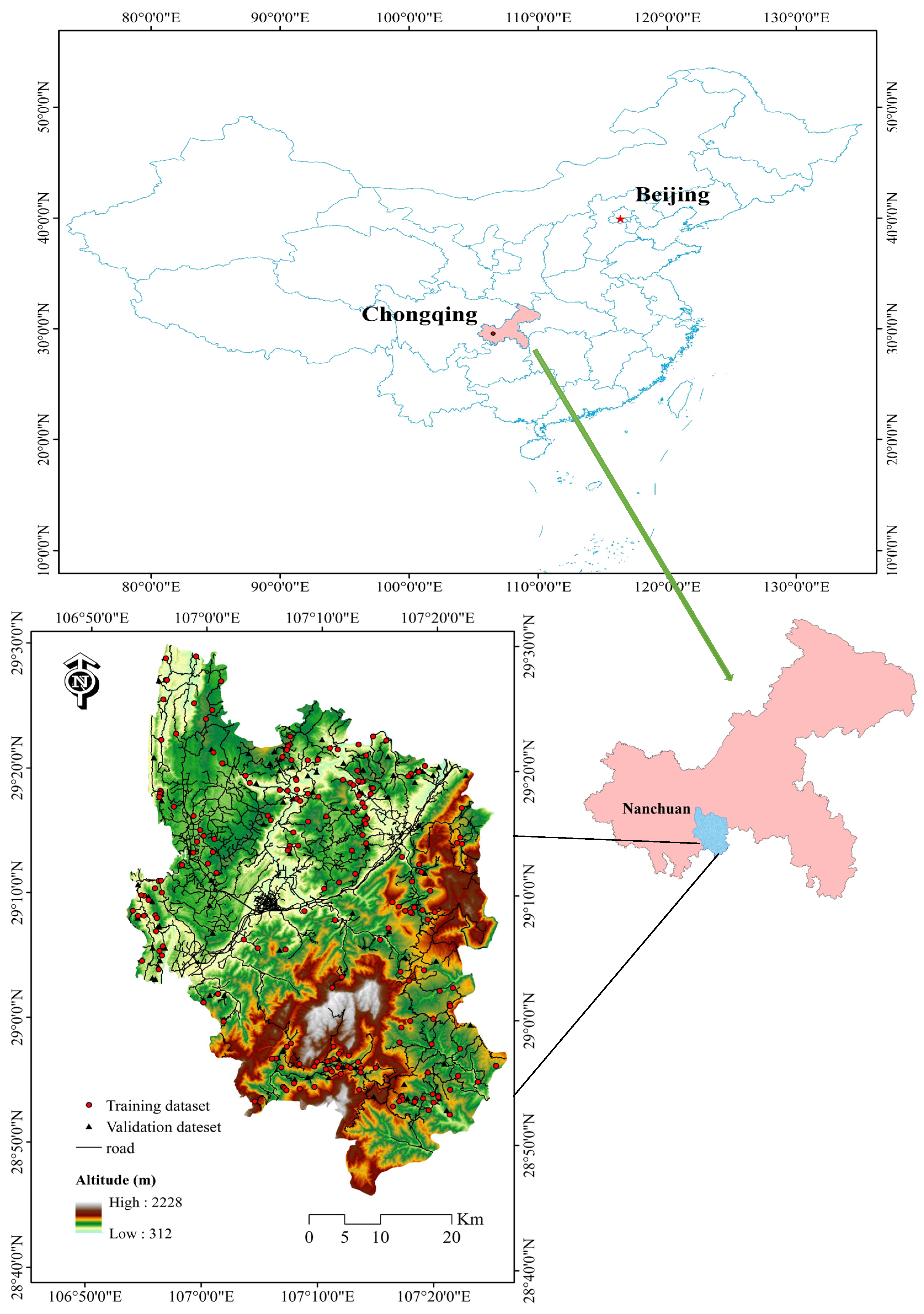
Nanchuan County is located within longitudes of 106°54′ E–107°27′ E and latitudes of 28°46′ N–29°30′ N (Figure 1). The study area has a subtropical humid monsoon climate with an annual average temperature of 20 °C, an average annual rainfall of 1172.20 mm, and an annual maximum rainfall of 1534.8 mm. The temporal distribution of atmospheric precipitation is extremely uneven, with a dry season that lasts for most of the year, and a rainy season in May, June, July, and August. Because of differences in structure, lithology, and neotectonic movement, the physiognomy in Nanchuan County is complex and diverse. In the urban area of Nanchuan County, the mountains are high, downcutting is strong, canyons are numerous, and the cliffs are steep, with obvious layers. Topographically, slopes less than 10° account for 1.91% of the total area, 10°–20° for 49.28%, 20–30° for 31.1%, 30–40° for 13.39%, 40–50° for 2.87%, and slopes over 50° for 1.43%.
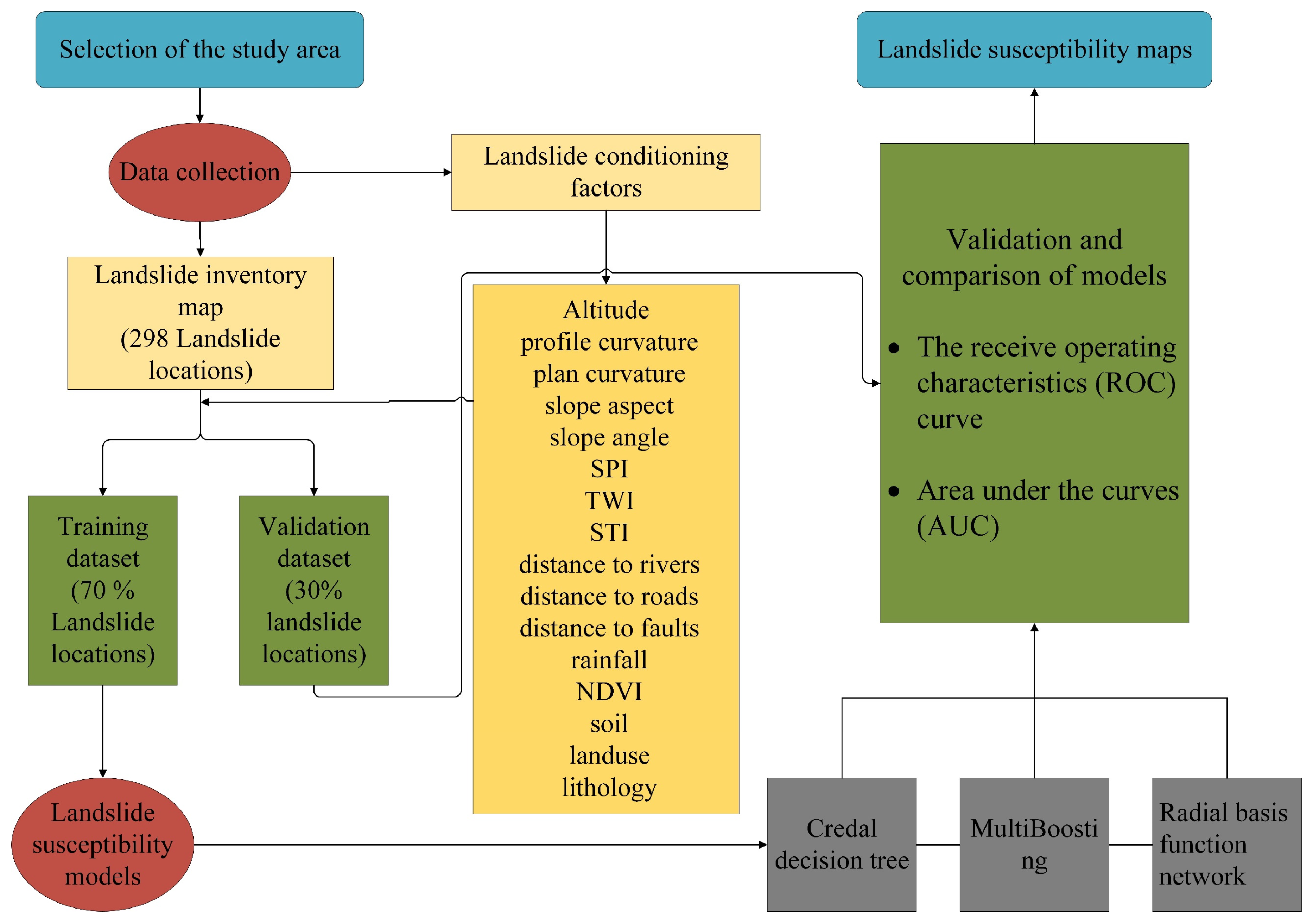
The research method of this study can be divided into the following five steps (Figure 2): (1) data collection; (2) generating the landslide inventory map and selecting factors; (3) establishing the landslide model; (4) validation and comparison of models; and (5) generating the landslide susceptibility map and determining the best model for the study area.
The landslide inventory, as the basis of landslide susceptibility mapping, includes the geographic locations of landslide occurrences [47]. The landslide inventory map also plays an important role in studying the relationships between landslide conditioning factors and landslides [29]. Studying the geological and climatic conditions related to landslides is helpful to predict the locations of future landslides in the area. Figure 1 shows the landslide inventory map of Nanchuan County based on a field geological survey and interpretation of aerial photos. Ultimately, 298 landslides were identified in the landslide inventory map. Following previous studies, the 298 landslides were randomly divided into two parts, 70% (209 landslides) for the training dataset and 30% (89 landslides) for the validation dataset. At the same time, the same number of non-landslide points were randomly selected in the study area and converted into pixels.
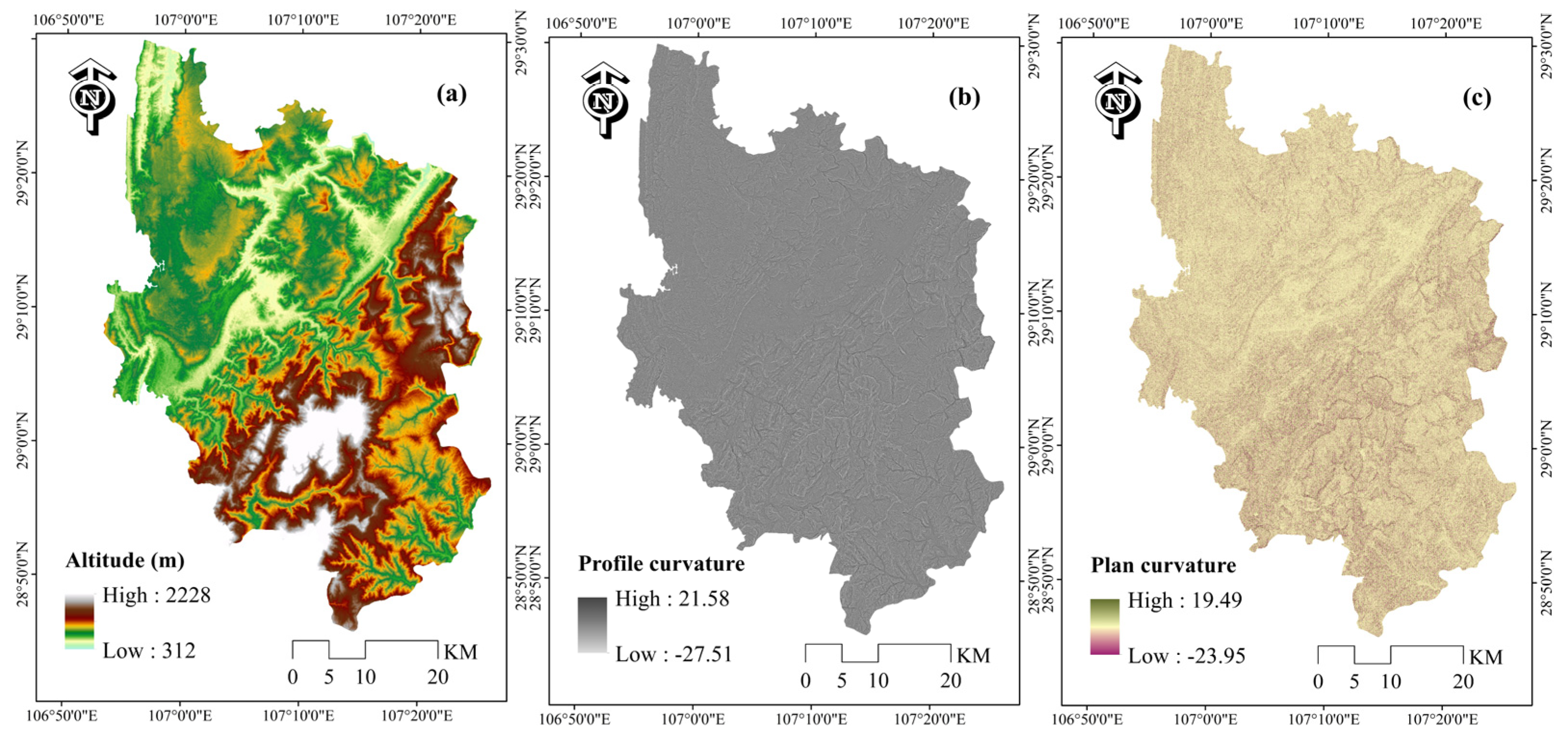
As the second step of generating the landslide susceptibility map, the landslide conditioning factors were determined. A digital elevation model (DEM) with a resolution of 20 m by 20 m was used to extract profile curvature, plan curvature, slope, aspect, stream power index (SPI), sediment transport index (STI), and topographic wetness index (TWI) factor maps. In this paper, a total of 16 landslide conditioning factors were determined according to relevant geological characteristics and environmental conditions for landslide susceptibility evaluation. Among the 16 landslide conditioning factors, 13 are continuous factors: Altitude, profile curvature, plan curvature, slope aspect, slope angle, SPI, TWI, STI, distance to rivers, distance to roads, distance to faults, rainfall, and normalized difference vegetation index (NDVI). The other three were categorical factors: Soil, land use, and lithology. Because the causes of landslides are not only complicated but also difficult to determine, the existing studies have not formed a unified choice of landslide conditioning factors [48]. However, previous studies have found the relationship between the occurrence of landslides and some conditions, such as topographic and geological characteristics, climatic conditions, and human activities [49]. Therefore, based on previous landslide susceptibility studies and related geological characteristics and environmental conditions in the study area, 16 landslide condition factors were determined. Finally, the 16 landslide conditioning factors were transformed into the same spatial resolution (20 by 20 m).
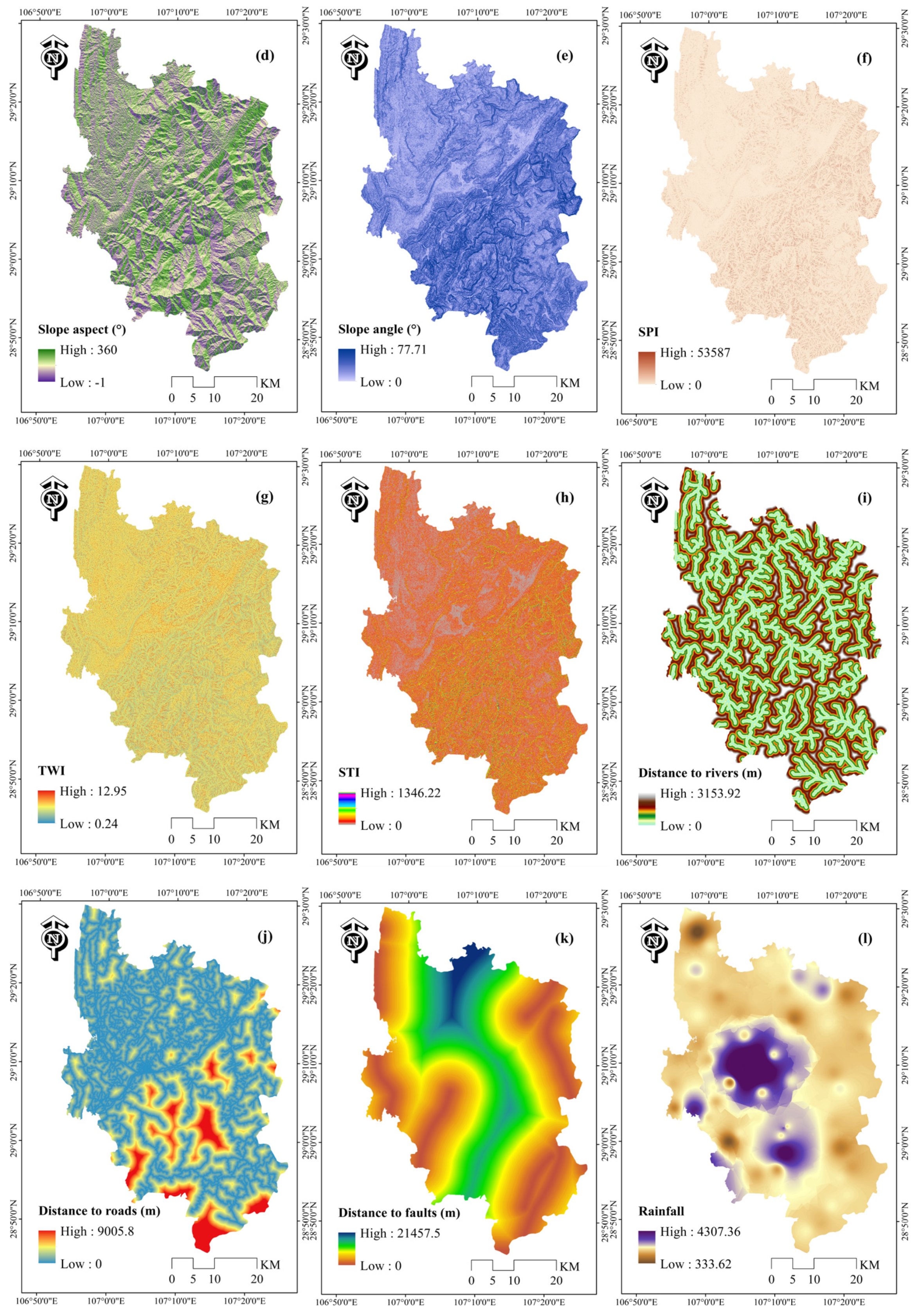
Nowadays, there is no accepted standard for the classification of landslide conditioning factors [50]. In this paper, classify the continuous factors based on the landslide distribution characteristics in the study area and refer to previous studies on landslide susceptibility analysis [51]. After referencing the literatures, all continuous factors are broken and classified in ArcGIS software [52]. Table 1 shows the classification list of factors in this study. Altitude is one of the important parameters in the study of landslide susceptibility and plays an important role in the evaluation. The study area has an altitude range of 312–2228 m, which was divided into nine categories at intervals of 200 m [53]. The vertical plane parallel to the inclined plane is called the profile curvature. The profile curvature influences the erosion and deposition of the slope by controlling the velocity of down-slope flows [54,55]. In this paper, the profile curvature ranges from −27.51 to 21.58 and is divided into three categories [56]. The profile curvature map was generated in the ArcGIS software (Figure 3b). Plan curvature influences the slope stability by controlling the dispersion and convergence of down-slope flows [57]. The plan curvature map was also generated in the ArcGIS software. The range of the plan curvature was −23.95–19.49, and these were divided into three categories [56]. Rainfall, solar exposure, and dry wind all affect the occurrence of landslides. All of these influencing parameters are related to slope aspect [58,59]. Therefore, slope aspect is also an important parameter in landslide susceptibility evaluation [60,61]. In this paper, the slope aspect was divided into nine categories [53]. The slope angle directly affects the occurrence of landslides; therefore, the slope angle is a parameter that cannot be ignored in landslide susceptibility evaluation [62,63,64,65], and is a factor frequently used in landslide susceptibility mapping [66,67]. The slope angle map of the study area was generated based on a DEM (Figure 3e), in which slope angles were divided into eight categories [53]. The SPI reflects the erosion capacity and sediment content of water flow. In this study, the SPI values were divided into five categories [68]. The TWI can reflect the water content in the soil, which is of great significance in the study of rock and soil stability. In this study, the TWI (0.24–12.95) was divided into five categories and mapped accordingly [20]. Figure 3h is the STI map, in which STI values were divided into five categories [69]: 0–5, 5–10, 10–15, 15–20, and >20.
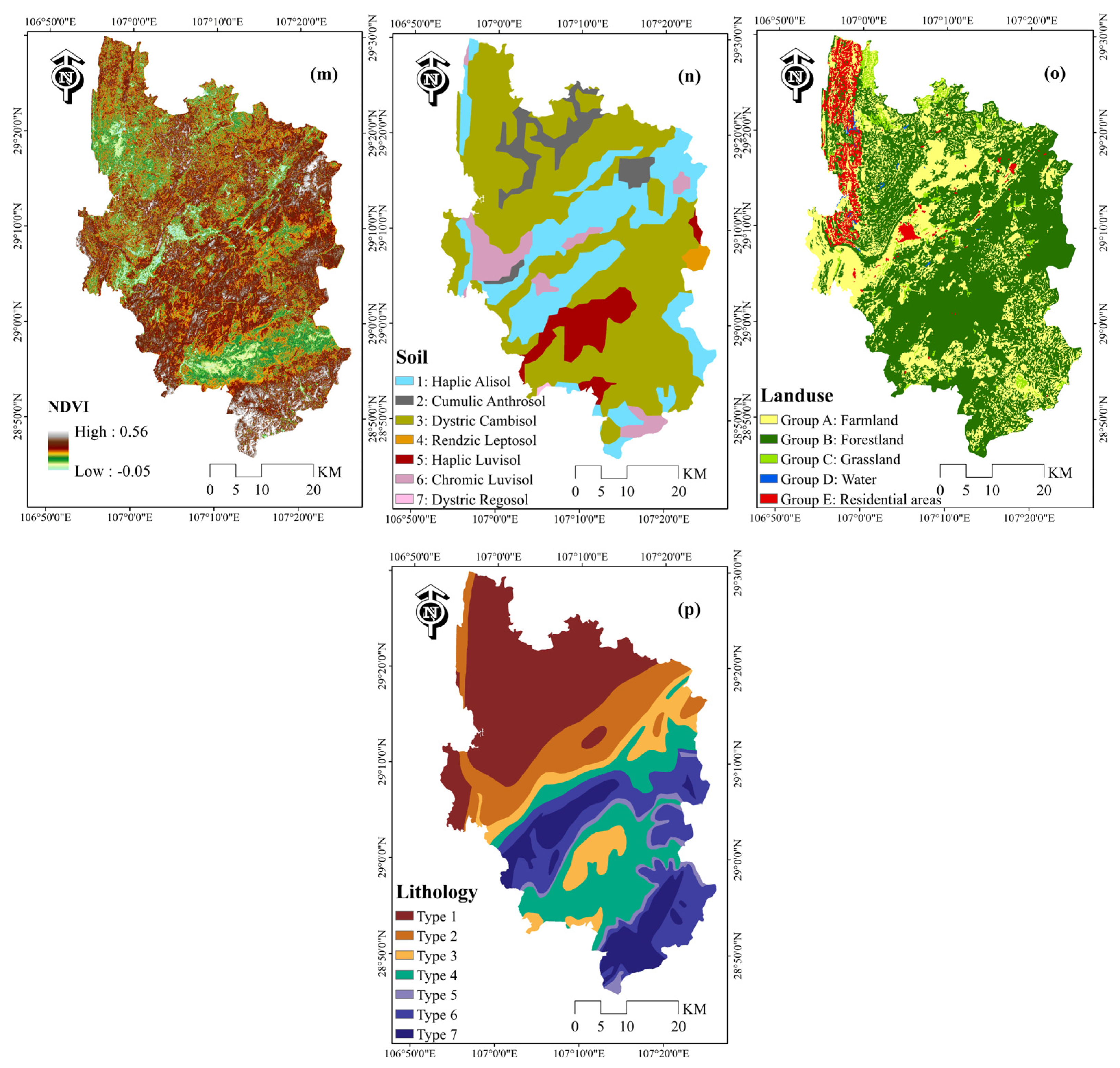
Rivers may influence the stability of a slope through erosion of the bottom of the slope and increasing the water level because of sediment accumulation at the bottom [64]. The distance to rivers was divided into five categories with intervals of 200 m [53]; the longest distance to a river in the study area was 3153.92 m. Building roads around slopes reduces the load on both the foot of the slope and the terrain; therefore, the distance to roads is a parameter that must be considered in landslide susceptibility mapping [64]. The range of distance to roads in the research area is 0–9005.8 m, which was also divided into five categories with an interval of 200 m [70]. Distance to faults is an important parameter in landslide susceptibility analysis. Faults are fractures of the earth’s crust, which reduce rock strength and can ultimately leads to landslides [71]. The distance to faults was divided into five categories: 0–1000 m; 1000–2000 m; 2000–3000 m; 3000–4000 m; and >4000 m [70]. These categories were mapped in the ArcGIS software. Rainfall, as one of the most important factor in inducing landslides, is also the most important factor in the evaluation of landslide susceptibility [72,73]. Rainfall in the study area was divided into five categories [74] in the generated rainfall map (Figure 3l). According to previous work, the NDVI value is directly proportional to the vegetation coverage area [75,76]. The range of NDVI values in the study area is −0.05–0.56. The NDVI map (Figure 3m) was generated and divided into five categories in the ArcGIS software [76]. Different soil types have different compositions and textures. In the study area, the soil map is divided into seven categories by soil type: Haplic Alisol, Cumulic Anthrosol, Dystric Cambisol, Rendzic Leptosol, Haplic Luvisol, Chromic Luvisol, and Dystric Regosol. Land use, as a landslide conditioning factor, can affect the stability of the slope. For example, the roots of vegetation can maintain the stability of the slope, thereby reducing the incidence of landslides [77]. Table 1 shows the land-use classification of the study area. Rock strength and permeability differ with different lithologies; therefore, the lithology influences landslide occurrence [78]. The lithological map of the study area shows classification into seven categories: Type 1 (Jurassic: Mudstone, sandstone, siltstone, and limestone), type 2 (Triassic: Limestone, dolomite, sandstone, and siltstone), type 3 (Permian: Limestone and shale with intercalation of siltstone), type 4 (Silurian: Shale, siltstone, and interbedded limestone), type 5 (Ordovician: Grayish-black charcoal shale with a siliceous base), type 6 (Ordovician: Limestone and carbonate), and type 7 (Cambrian: Dolomite and limestone).
3. Modeling Approach
3.1. Credal Decision Tree
Credal decision trees are used to solve classification problems of credal sets [79]. Compared with the J48 algorithm, which uses information gain as the segmentation standard to determine the attributes of each branch node, a CDT considers the imprecise probability and uncertainty in the original segmentation standards [79]. The processing method of missing values is the same as that of C4.5 [80]. The measure of total uncertainty (TU) consists of two parts, which can be expressed as [41,79]:
where φ represents a credal set on a frame X, TU is the value of the total uncertainty, IG represents a non-specific general function on the corresponding credal set, and GG is a general function of the randomness of credal sets.
The function of the non-specific state can be expressed as [79]:
where m (φ) is a focal element and A is the power set of X.
The measure of the randomness of a general credal set can be expressed as [79]:
where the maximum occupies all probability distributions of φ and φ represents a general credal set. This function not only verifies all the basic properties verified in Dempster–Shafer’s theory but also is a good measure of the randomness for credal sets [79,81].
3.2. Radial Basis Function Network
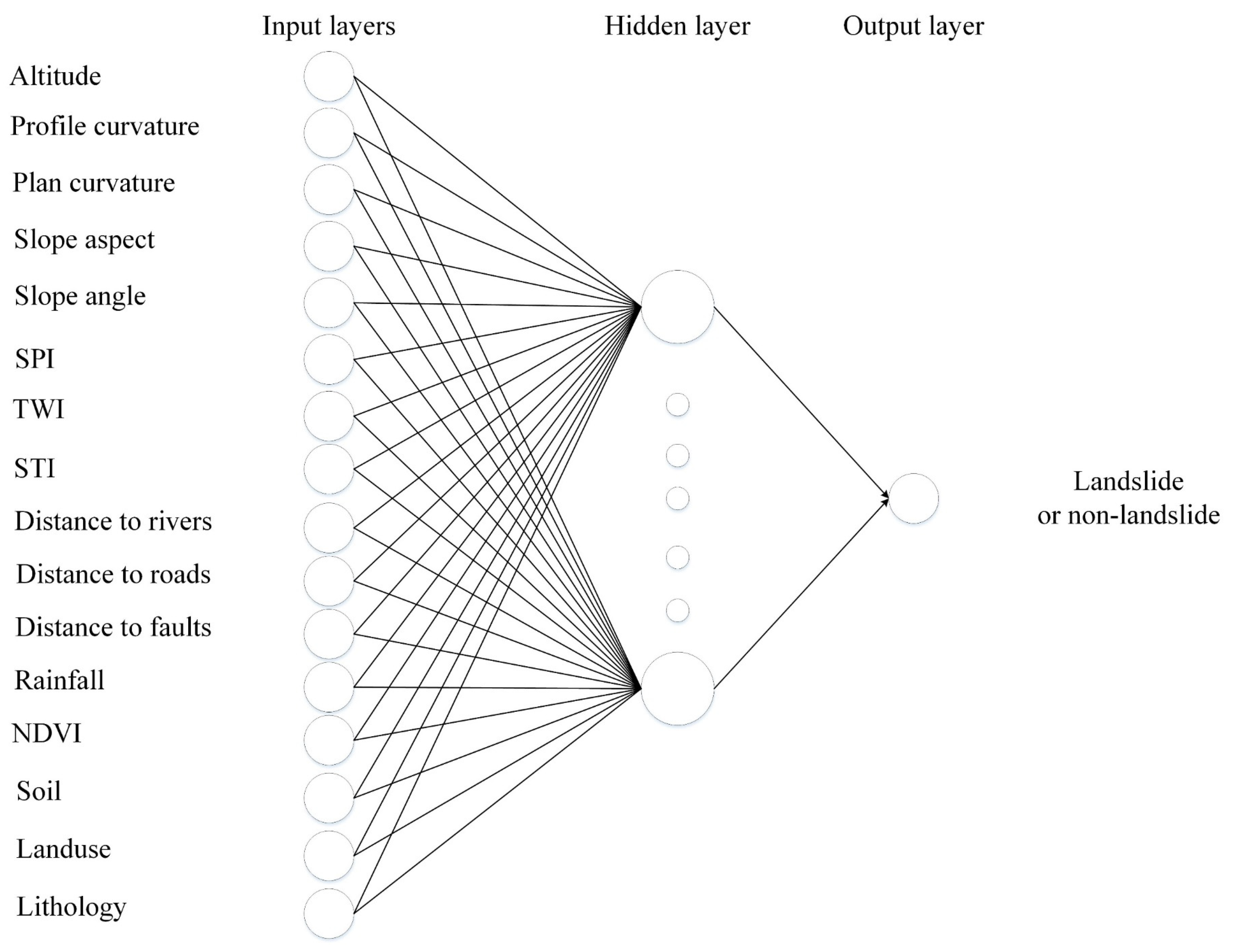
Radial basis function networks are an effective method to solve nonlinear problems using a special radial function [82]. These networks are now widely used in various fields, such as image processing and analysis [83,84] and credit estimation [85]. In this paper, Figure 4 shows the framework structure of the RBFN, which consists of 16 input layers, a hidden layer, and an output layer. The mapping from the output layer to the hidden layer is non-linear, whereas the mapping from the hidden layer to the output layer is linear [86]. Finally, the output layer can be expressed as in Equation (4) [86]:
where n is the number of nodes of the hidden point, ci represents the center of the ith hidden node, x is the input vector, wih is the weight of the ith node of the hidden layer, w0h is the offset of the h node of the output layer, and is the radial basis function centered on ci. In general, the Gaussian function is often used as a basis function in RBFN. The Gaussian function can be expressed as in Equation (5) [86]:
where x indicates the input vector and ci indicates the center vector of the ith hidden node of the RBFN.
3.3. MultiBoosting
MultiBoost is a combination of AdaBoost and wagging, and is an extension of the AdaBoost technique for forming decision committees [87]. Decision committee learning can reduce the misclassification of learning classifiers [88]. It has been found that MultiBoost can reduce most of AdaBoost’s superior bias while reducing most of the superior variance of bagging [88]. MultiBoost not only has the bias and variance reduction features in its constituent committee learning algorithm, but also has a potential computational advantage: Committees can learn in parallel [88].
The working principle of the MultiBoost method can be divided into three steps: First, a subset is randomly selected from the training dataset to generate the initial base classifier; then, the instance weight is adjusted according to the precision performance of the base classifier; and finally, a new subset is selected from the weighted instance to train a new classifier [89]. For the training dataset S (xi, yi), where xi ∈ R, yi ∈ (landslide, non-landslide), the final classifier can be obtained from the following equations [46]:
where S′ is S with instance weights assigned to be 1, Ct is a base learner (S′), and εt is the weighted error on the training dataset.
4. Results
4.1. Optimization of the Dataset
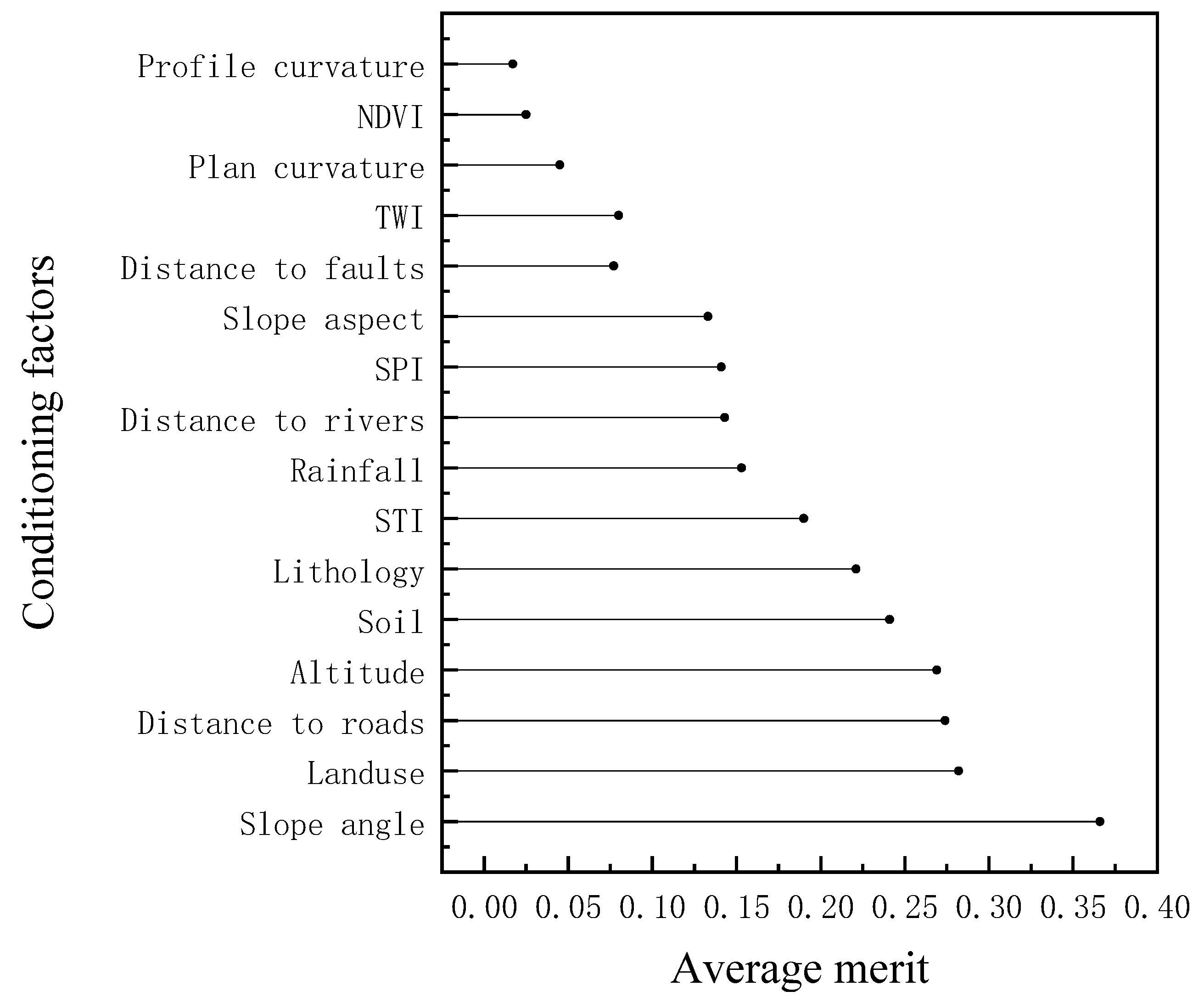
In this paper, the correlation attributes evaluation (CAE) method was used to study the influence of each landslide conditioning factor on landslide occurrence [90]. The calculated average merit (AM) values reflect the influence ability of the selected factors; a greater AM value indicates greater influence [43,91]. The AM values of the 16 conditioning factors evaluated in the study area were calculated as follows: Altitude, 0.269; profile curvature, 0.017; plan curvature, 0.045; slope aspect, 0.133; slope angle, 0.366; SPI, 0.143; TWI, 0.08; STI, 0.19; distance to rivers, 0.141; distance to roads, 0.274; distance to faults, 0.077; rainfall, 0.153; NDVI, 0.025; soil, 0.241; land use, 0.282; and lithology, 0.221 (Figure 5).
4.2. Model Performances and Validation
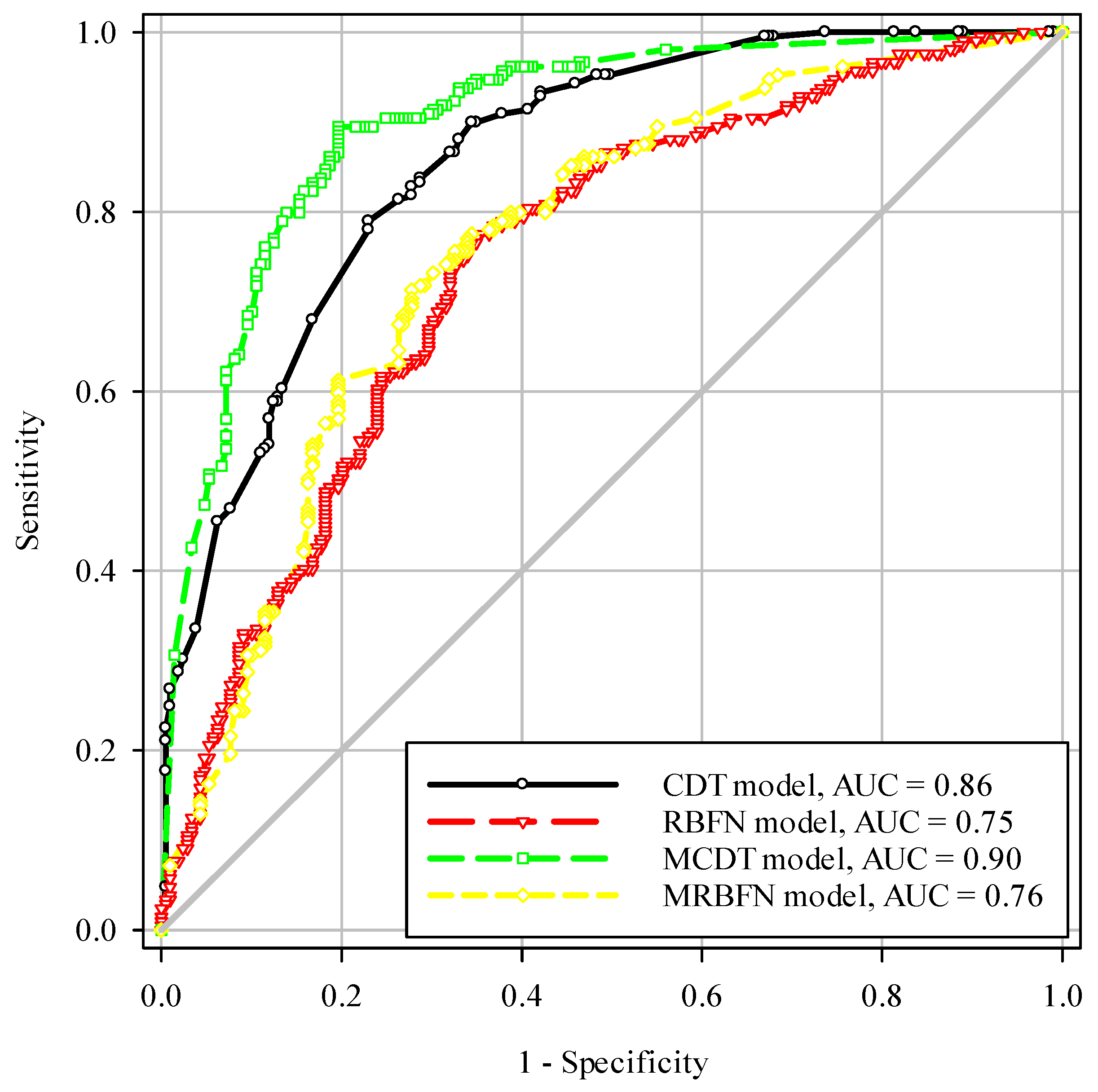
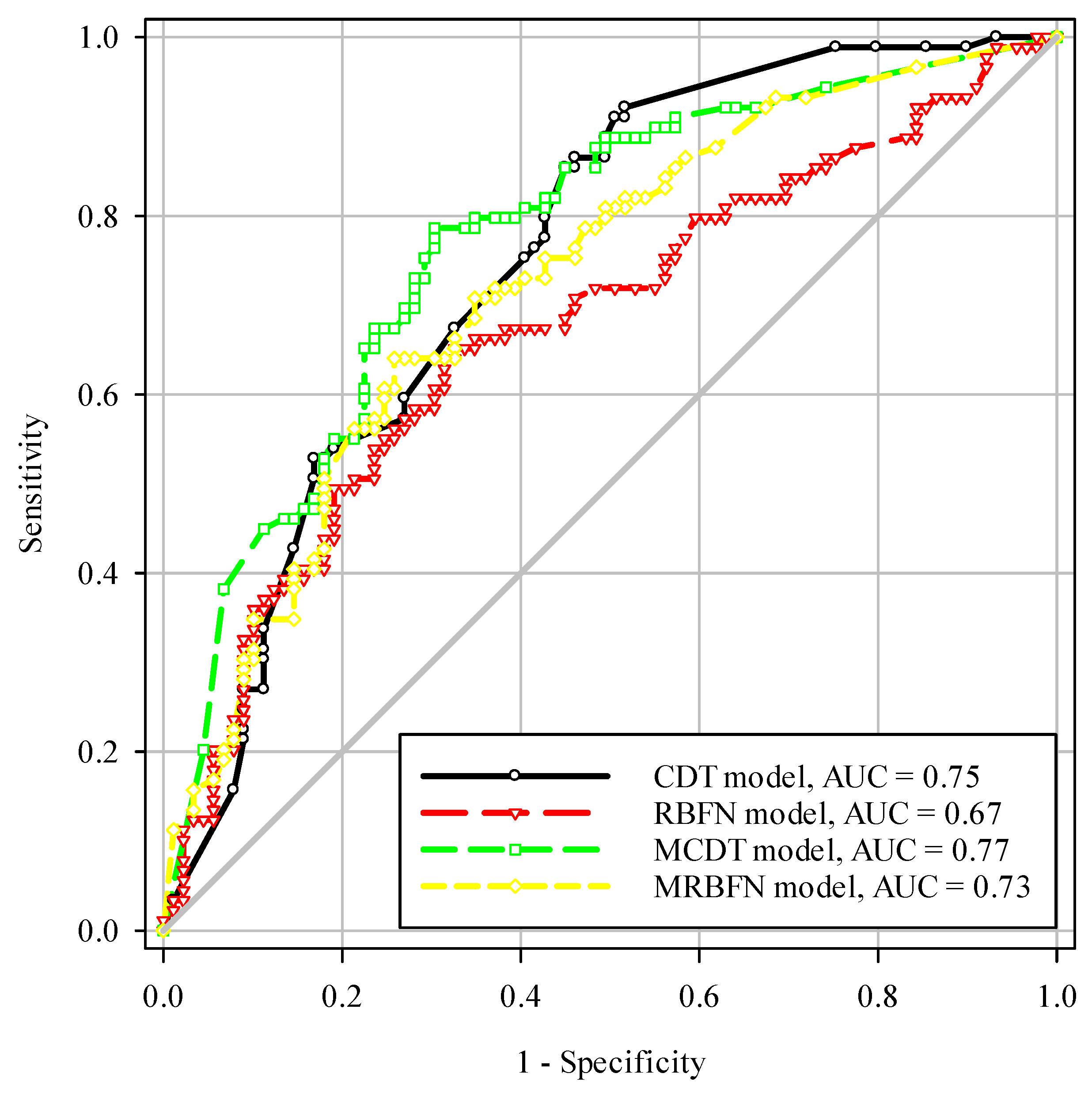
The main purpose of landslide susceptibility evaluation is to identify locations that may be affected by future landslides [29]. Therefore, no matter which integration method is used to generate the landslide susceptibility map, it needs to be verified and evaluated [92]. In this paper, a popular technique called the area under the ROC curve (AUC) was used to quantitatively determine the predictive power of two integrated models and the two single models [93,94,95,96]. The ROC curve was plotted using the sensitivity and 1-specificity of the model [97]. Figure 6 shows the AUC values based on the training dataset. Both the single model and the integrated model had good predictive power. The AUC values of the CDT, RBFN, MultiBoosting CDT (MCDT), and MRBFN models are 0.86, 0.75, 0.90, and 0.76, respectively. However, the performance of the MCDT model was optimal (AUC = 0.90). When validating a model, the AUC value based on the training data set cannot be considered separately. The AUC values for the validation dataset were not used to construct the model but should be considered for verifying the model. Figure 7 shows the AUC values using the validation dataset. The AUC values of the CDT, RBFN, MCDT, and MRBFN models are 0.75, 0.67, 0.77, and 0.73, respectively. Based on the verification data, the MCDT model still had the best performance (AUC = 0.77).
Table 2 and Table 3 show three evaluation statistics that were used in addition to the AUC values: The standard error, 95% confidence interval (CI), and significance level (p-value). These statistical methods were used to verify and compare the performance of the models. In general, smaller standard error values, smaller CI, and smaller p-values indicate better model performance [91]. The MCDT model not only produced the minimum standard errors, 95% CI, and p-values in the training and validation datasets but also yielded the highest AUC value, indicating that the performance of the MCDT model was the best in this study.
The chi-square test was used to verify the performance of the four models (CDT, RBFN, MCDT, and MRBFN) through pairwise comparison. Table 4 shows the level of significance after comparison. The chi-square values of five groups were significantly higher than the critical value of 3.841, and the significance level was also higher than the critical value of 0.05. However, the RBFN model and MRBFN model differed from other models. In particular, the significance levels of the MCDT and RBFN models are notable. Through comparison, it was found that there were statistical differences between all models except the RBFN and MRBFN models.
4.3. Generation of Landslide Susceptibility Maps
The characteristic of CDT is that it does not ignore imprecise probabilities and the application of uncertainty measures for the original split criterion [79]. It not only reduces wrong pruning by back fitting but also sorted values for numeric attributes. Furthermore, it treats missing values and values similarly to C4.5. The parameters used in the construction of the CDT model are: Svalue is 1.0, maxDepth is −1, minNum is 2.0, numFolds is 3, and seed is 1. The RBFN model is established based on the training data. The ten-fold cross-validation method used in Weka software [98] not only reduces the variability of the model, but also avoids the problem of overfitting in the modeling process. The parameters used in the RBFN model are: Clustering seed is 1, maximum number of iterations is −1, the number of clusters is 2, minimum standard deviation is 0.1, and ridge is 1.0E-8. The function of the MultiBoosting algorithm in the modeling process is to use the training subset to construct various classifier-based models, and then adjust the weights of the classifier-based models to optimize the classification accuracy. The advantage of using MultiBoosting to build a hybrid model is that MultiBoost symmetrically considers the characteristics of Boosting and wagging to prevent overfitting problems [89]. Besides, the accuracy of classification results can be increased by reducing the variance and deviation of the system. The parameters used by the MultiBoosting model are: Numlterations is 10, numSubCmtys is 3, seed is 1, and weightThreshold is 100.
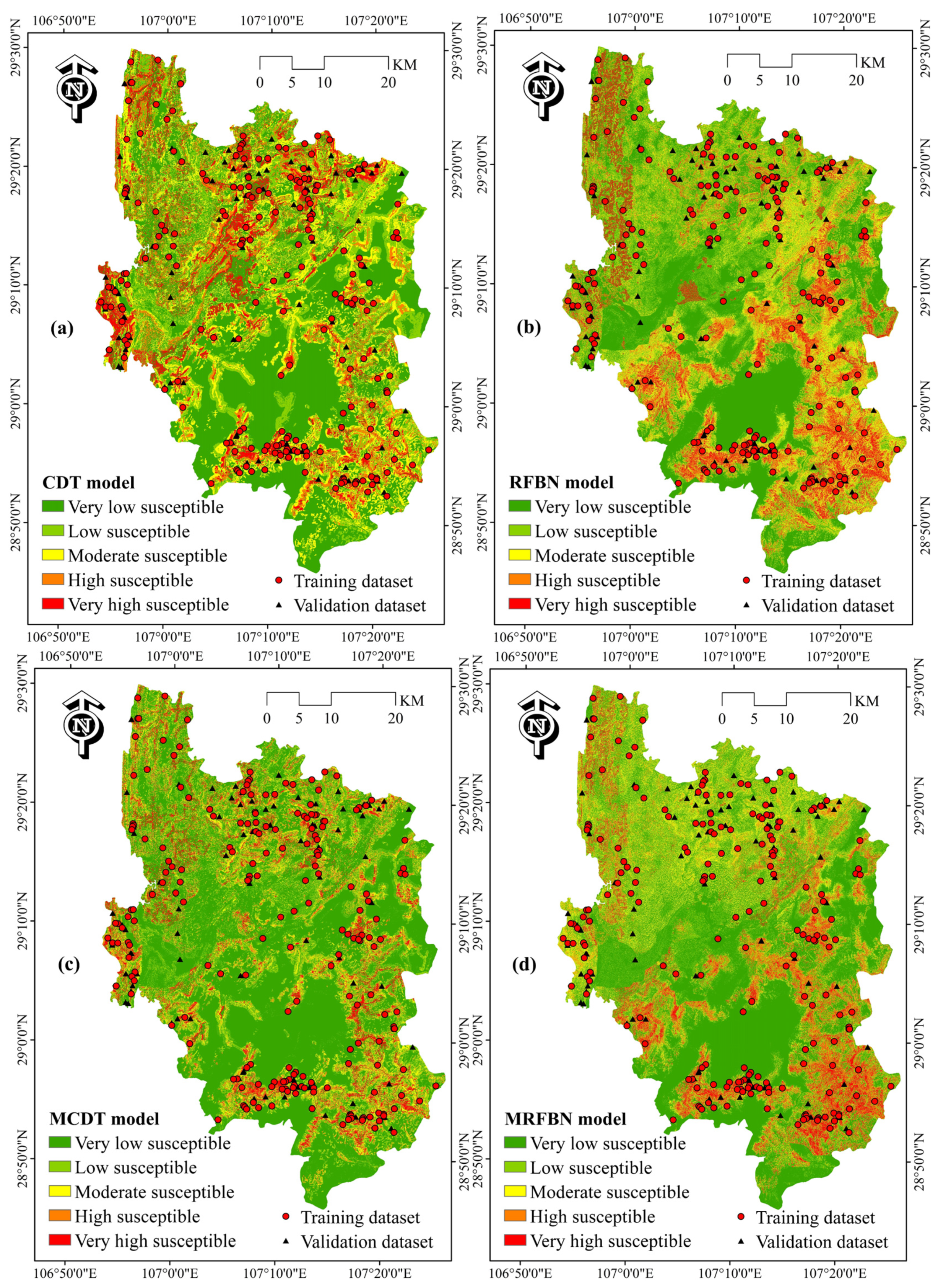
When the training and validation of the models were completed, the models were applied to the study area to calculate the landslide susceptibility indices (LSI). The LSI values were then converted to raster format to generate landslide susceptibility maps in the ArcGIS software. Figure 8a–d shows the landslide susceptibility maps constructed using the CDT, RBFN, MCDT, and MRBFN models, respectively. The corresponding LSI value ranges of the four landslide susceptibility maps are 0.039 to 0.949, 0.092 to 0.852, 0 to 1, and 0 to 1. Using the equal area method, each of the four landslide susceptibility maps was divided into five landslide susceptibility classes: Very low (40%), low (20%), moderate (20%), high (10%), and very high susceptibility (10%), for better comparison of the landslide susceptibility maps. The susceptibility zones of the landslides can be visually assessed from the four figures.
5. Discussions
In this paper, two hybrid models of MultiBoosting-based artificial intelligence methods were established: The MCDT and MRBFN models. The main purpose was to evaluate landslide susceptibility in Nanchuan County, China. To build the landslide susceptibility models, 16 landslide conditioning factors were determined.
The results show that each conditioning factor contributed to the modeling of landslide susceptibility, but the extents of their contributions differed. Slope angle yielded the highest AM value, which demonstrates the importance of slope angle to landslide susceptibility. In addition, altitude is an important factor that also produced a high AM value in the landslide susceptibility evaluation. Soils with different compositions and structures affect landslide occurrences [18], and the AM values show that soil types play an important role in this study area. Road construction will destroy the natural topology and make slopes unstable. Therefore, distance to roads has become an important factor affecting landslides. In this study, distance to roads (AM = 0.274) occupies a relatively high position in the overall landslide conditioning. Rainfall is also one of the main parameters in landslide susceptibility evaluation and is closely related to landslide occurrence. The rainy season in the study area lasts for four months: May, June, July, and August. The maximum daily rainfall in the area is 121.4 mm. Rainfall (AM = 0.153) is an essential parameter for landslide susceptibility assessment in the study area. Lithology and land use, both important parameters in landslide studies [61,99], also play important roles in this study area. Based on the AM values of plan curvature, TWI, NDVI, and profile curvature, it can be inferred that the occurrence of landslides is less affected by these four factors in the study area, as these factors had no significant influence (AM < 0.01) on landslide occurrence. However, these factors cannot be ignored because many scholars have studied their relationships with landslides.
Visual analysis of the four landslide susceptibility maps revealed the same very low susceptibility zone around the southwest valley. However, the southeast of the study area is covered by areas of high and very high susceptibility. Figure 8 shows that the four landslide susceptibility maps have similar spatial distributions of moderate and high susceptibility zones. In this study, the target ratio of the hybrid models was smaller than that of the single models under visual analysis. For the two single models, this means that the hybrid models had higher predictive power and reliability.
The performances of the two-hybrid models and the two single models were verified and compared. Performance of the two-hybrid models was significantly improved compared with the single models under the training dataset and the validation dataset. Based on comparison of the ROC curves, SEs, and 95% CI of the two hybrid models, the MCDT model performed better than the MRBFN model. The final results show that the MCDT model had the best performance in this study, with the minimum SE (0.015) and CI (0.87–0.93) and maximum AUC (0.90) under the training dataset, as well as the minimum SE (0.035) and CI (0.71–0.84) and maximum AUC (0.77) under the validation dataset. These four landslide susceptibility maps will help local government agencies and related organizations to prevent and manage landslide hazards. All models and methods used in this study can be used to evaluate landslide susceptibility in other areas with similar conditions.
6. Conclusions
The main purpose of this study was to apply MultiBoosting with two artificial intelligence methods (the RBFN and CDT models) to evaluate landslide susceptibility in Nanchuan County, China. A total of 16 landslide conditioning factors (altitude, profile curvature, plan curvature, slope aspect, slope angle, SPI, TWI, STI, distance to rivers, distance to roads, distance to faults, rainfall, NDVI, soil, land use, and lithology) were determined to affect the occurrence of landslides in the study area. The landslide susceptibility maps generated by the two-hybrid models and those generated by the two single models were compared in pairs. ROC curves, statistical analysis methods, and chi-square tests were used to compare and evaluate the spatial prediction abilities of the hybrid models and single models.
The final results show that both the hybrid model and the single model contributed to the evaluation of landslide susceptibility in the study area, but the evaluation capabilities were different. The AUC values of the CDT, RBFN, MCDT, and MRBFN models were 0.75, 0.67, 0.77, and 0.73, respectively. These results indicate that the hybrid models MCDT and MRBFN had higher predictive power than the CDT model and RBFN model. However, the MCDT model had the best performance in the study area. Through this research, it can be concluded that a hybrid model can improve the predictive ability of a single model. The hybrid models used in this study can be employed to help prevent and control landslide disasters in similar areas.
The final results show that two hybrid computational intelligence methods (MCDT and MRBFN) can be successfully applied to landslide susceptibility assessment. The obtained landslide susceptibility map can provide valuable information for local governments or organizations to study slope stability and can also be used as a reference for infrastructure planning, engineering design and disaster reduction design. However, the best method for landslide susceptibility mapping still needs to be studied and discussed in this study area. Therefore, it is recommended to carry out detailed land use planning and urban development after specific site surveys in very high and highly sensitive areas.
Author Contributions
G.W., X.L., W.C., H.S. and A.S. contributed equally to the work. X.L. and G.W. collected field data and conducted the landslide susceptibility mapping and analysis. X.L. and W.C. wrote and revised the manuscript. G.W., H.S. and A.S. provided critical comments in planning this paper and edited the manuscript. All the authors discussed the results and edited the manuscript. All authors have read and agreed to the published version of the manuscript.
Funding
This study was supported by the National Natural Science Foundation of China (41807192), Natural Science Basic Research Program of Shaanxi (Program No. 2019JLM-7, Program No. 2019JQ-094), China Postdoctoral Science Foundation (Grant No. 2018T111084, 2017M613168), and Project funded by Shaanxi Province Postdoctoral Science Foundation (Grant No. 2017BSHYDZZ07).
Acknowledgments
Great thanks are given to Xingguang Chen and Zhengqian Wu for their kind help.
Conflicts of Interest
The authors declare no conflict of interest.
References
- Tien Bui, D.; Pradhan, B.; Lofman, O.; Revhaug, I.; Dick, O.B. Landslide susceptibility assessment in the Hoa Binh province of Vietnam: A comparison of the Levenberg–Marquardt and Bayesian regularized neural networks. Geomorphology 2012, 171, 12–29. [Google Scholar] [CrossRef]
- Pradhan, B.; Youssef, A.M. Manifestation of remote sensing data and GIS on landslide hazard analysis using spatial-based statistical models. Arab. J. Geosci. 2010, 3, 319–326. [Google Scholar] [CrossRef]
- Zêzere, J.L.S.; de Brum Ferreira, A.; Rodrigues, M.L.S. The role of conditioning and triggering factors in the occurrence of landslides: A case study in the area north of lisbon (portugal). Geomorphology 1999, 30, 133–146. [Google Scholar] [CrossRef]
- Fernandes, A.M.; Utkin, A.B.; Lavrov, A.V.; Vilar, R.M. Development of neural network committee machines for automatic forest fire detection using lidar. Pattern Recognit. 2004, 37, 2039–2047. [Google Scholar] [CrossRef]
- Cubito, A.; Ferrara, V.; Pappalardo, G. Landslide hazard in the nebrodi mountains (northeastern sicily). Geomorphology 2005, 66, 359–372. [Google Scholar] [CrossRef]
- Moreiras, S.M. Landslide susceptibility zonation in the rio mendoza valley, argentina. Geomorphology 2005, 66, 345–357. [Google Scholar] [CrossRef]
- Constantin, M.; Bednarik, M.; Jurchescu, M.C.; Vlaicu, M. Landslide susceptibility assessment using the bivariate statistical analysis and the index of entropy in the Sibiciu Basin (Romania). Environ. Earth Sci. 2011, 63, 397–406. [Google Scholar] [CrossRef]
- Guzzetti, F.; Reichenbach, P.; Ardizzone, F.; Cardinali, M.; Galli, M. Estimating the quality of landslide susceptibility models. Geomorphology 2006, 81, 166–184. [Google Scholar] [CrossRef]
- Van Westen, C. Geo-information tools for landslide risk assessment: An overview of recent developments. Landslides Eval. Stab. 2004, 1, 39–56. [Google Scholar]
- Runqiu, H. Large-scale landslides and their sliding mechanisms in China since the 20th century. Chin. J. Rock Mech. Eng. 2007, 26, 433–454. [Google Scholar]
- Chen, H.; Zeng, Z.; Tang, H. Landslide deformation prediction based on recurrent neural network. Neural Process. Lett. 2015, 41, 169–178. [Google Scholar] [CrossRef]
- Guo, C.; Qin, Y.; Ma, D.; Xia, Y.; Chen, Y.; Si, Q.; Lu, L. Ionic composition, geological signature and environmental impacts of coalbed methane produced water in China. Energy Sources Part A Recovery Util. Environ. Eff. 2019, 1–15. [Google Scholar] [CrossRef]
- Pradhan, B. Landslide susceptibility mapping of a catchment area using frequency ratio, fuzzy logic and multivariate logistic regression approaches. J. Indian Soc. Remote Sens. 2010, 38, 301–320. [Google Scholar] [CrossRef]
- Zhao, X.; Chen, W. GIS-based evaluation of landslide susceptibility models using certainty factors and functional trees-based ensemble techniques. Appl. Sci. 2020, 10, 16. [Google Scholar] [CrossRef] [Green Version]
- Chen, W.; Hong, H.; Panahi, M.; Shahabi, H.; Wang, Y.; Shirzadi, A.; Pirasteh, S.; Alesheikh, A.A.; Khosravi, K.; Panahi, S.; et al. spatial prediction of landslide susceptibility using GIS-based data mining techniques of ANFIS with Whale Optimization Algorithm (WOA) and Grey Wolf Optimizer (GWO). Appl. Sci. 2019, 9, 3755. [Google Scholar] [CrossRef] [Green Version]
- Gorsevski, P.V.; Brown, M.K.; Panter, K.; Onasch, C.M.; Simic, A.; Snyder, J. Landslide detection and susceptibility mapping using LiDAR and an artificial neural network approach: A case study in the Cuyahoga Valley National Park, Ohio. Landslides 2016, 13, 467–484. [Google Scholar] [CrossRef]
- Wang, L.-J.; Guo, M.; Sawada, K.; Lin, J.; Zhang, J. A comparative study of landslide susceptibility maps using logistic regression, frequency ratio, decision tree, weights of evidence and artificial neural network. Geosci. J. 2016, 20, 117–136. [Google Scholar] [CrossRef]
- Pham, B.T.; Bui, D.T.; Pourghasemi, H.R.; Indra, P.; Dholakia, M. Landslide susceptibility assesssment in the Uttarakhand area (India) using GIS: A comparison study of prediction capability of naïve bayes, multilayer perceptron neural networks, and functional trees methods. Theor. Appl. Climatol. 2017, 128, 255–273. [Google Scholar] [CrossRef]
- Tsangaratos, P.; Ilia, I. Comparison of a logistic regression and Naïve Bayes classifier in landslide susceptibility assessments: The influence of models complexity and training dataset size. Catena 2016, 145, 164–179. [Google Scholar] [CrossRef]
- He, Q.; Shahabi, H.; Shirzadi, A.; Li, S.; Chen, W.; Wang, N.; Chai, H.; Bian, H.; Ma, J.; Chen, Y.; et al. Landslide spatial modelling using novel bivariate statistical based Naïve Bayes, RBF Classifier, and RBF Network machine learning algorithms. Sci. Total Environ. 2019, 663, 1–15. [Google Scholar] [CrossRef]
- Huang, Y.; Zhao, L. Review on landslide susceptibility mapping using support vector machines. Catena 2018, 165, 520–529. [Google Scholar] [CrossRef]
- Kumar, D.; Thakur, M.; Dubey, C.S.; Shukla, D.P. Landslide susceptibility mapping & prediction using support vector machine for Mandakini River Basin, Garhwal Himalaya, India. Geomorphology 2017, 295, 115–125. [Google Scholar]
- Lin, G.-F.; Chang, M.-J.; Huang, Y.-C.; Ho, J.-Y. Assessment of susceptibility to rainfall-induced landslides using improved self-organizing linear output map, support vector machine, and logistic regression. Eng. Geol. 2017, 224, 62–74. [Google Scholar] [CrossRef]
- Zhao, Y.; Wang, R.; Jiang, Y.; Liu, H.; Wei, Z. GIS-based logistic regression for rainfall-induced landslide susceptibility mapping under different grid sizes in Yueqing, Southeastern China. Eng. Geol. 2019, 105147. [Google Scholar] [CrossRef]
- Yang, J.; Song, C.; Yang, Y.; Xu, C.; Guo, F.; Xie, L. New method for landslide susceptibility mapping supported by spatial logistic regression and GeoDetector: A case study of Duwen Highway Basin, Sichuan Province, China. Geomorphology 2019, 324, 62–71. [Google Scholar] [CrossRef]
- Aditian, A.; Kubota, T.; Shinohara, Y. Comparison of GIS-based landslide susceptibility models using frequency ratio, logistic regression, and artificial neural network in a tertiary region of Ambon, Indonesia. Geomorphology 2018, 318, 101–111. [Google Scholar] [CrossRef]
- Li, Y.; Chen, W. Landslide susceptibility evaluation using hybrid integration of evidential belief function and machine learning techniques. Water 2020, 12, 113. [Google Scholar] [CrossRef] [Green Version]
- Hong, H.; Ilia, I.; Tsangaratos, P.; Chen, W.; Xu, C. A hybrid fuzzy weight of evidence method in landslide susceptibility analysis on the Wuyuan area, China. Geomorphology 2017, 290, 1–16. [Google Scholar] [CrossRef]
- Mohammady, M.; Pourghasemi, H.R.; Pradhan, B. Landslide susceptibility mapping at Golestan Province, Iran: A comparison between frequency ratio, Dempster–Shafer, and weights-of-evidence models. J. Asian Earth Sci. 2012, 61, 221–236. [Google Scholar] [CrossRef]
- Dahal, R.K.; Hasegawa, S.; Nonomura, A.; Yamanaka, M.; Dhakal, S.; Paudyal, P. Predictive modelling of rainfall-induced landslide hazard in the Lesser Himalaya of Nepal based on weights-of-evidence. Geomorphology 2008, 102, 496–510. [Google Scholar] [CrossRef]
- Chen, W.; Shahabi, H.; Shirzadi, A.; Hong, H.; Akgun, A.; Tian, Y.; Liu, J.; Zhu, A.X.; Li, S. Novel hybrid artificial intelligence approach of bivariate statistical-methods-based kernel logistic regression classifier for landslide susceptibility modeling. Bull. Eng. Geol. Environ. 2019, 78, 4397–4419. [Google Scholar] [CrossRef]
- Khan, H.; Shafique, M.; Khan, M.A.; Bacha, M.A.; Shah, S.U.; Calligaris, C. Landslide susceptibility assessment using Frequency Ratio, a case study of northern Pakistan. Egypt. J. of Remote Sens. Space Science 2019, 22, 11–24. [Google Scholar] [CrossRef]
- Yan, F.; Zhang, Q.; Ye, S.; Ren, B. A novel hybrid approach for landslide susceptibility mapping integrating analytical hierarchy process and normalized frequency ratio methods with the cloud model. Geomorphology 2019, 327, 170–187. [Google Scholar] [CrossRef]
- Shahabi, H.; Khezri, S.; Ahmad, B.B.; Hashim, M. Landslide susceptibility mapping at central Zab basin, Iran: A comparison between analytical hierarchy process, frequency ratio and logistic regression models. Catena 2014, 115, 55–70. [Google Scholar] [CrossRef]
- Chen, W.; Fan, L.; Li, C.; Pham, B.T. Spatial Prediction of Landslides Using Hybrid Integration of Artificial Intelligence Algorithms with Frequency Ratio and Index of Entropy in Nanzheng County, China. Appl. Sci. 2020, 10, 29. [Google Scholar] [CrossRef] [Green Version]
- Althuwaynee, O.F.; Pradhan, B.; Lee, S. A novel integrated model for assessing landslide susceptibility mapping using CHAID and AHP pair-wise comparison. Int. J. Remote Sens. 2016, 37, 1190–1209. [Google Scholar] [CrossRef]
- Umar, Z.; Pradhan, B.; Ahmad, A.; Jebur, M.N.; Tehrany, M.S. Earthquake induced landslide susceptibility mapping using an integrated ensemble frequency ratio and logistic regression models in West Sumatera Province, Indonesia. Catena 2014, 118, 124–135. [Google Scholar] [CrossRef]
- Pham, B.T.; Khosravi, K.; Prakash, I. Application and comparison of decision tree-based machine learning methods in landside susceptibility assessment at Pauri Garhwal Area, Uttarakhand, India. Environ. Process. 2017, 4, 711–730. [Google Scholar] [CrossRef]
- Chen, W.; Li, H.; Hou, E.; Wang, S.; Wang, G.; Panahi, M.; Li, T.; Peng, T.; Guo, C.; Niu, C.; et al. GIS-based groundwater potential analysis using novel ensemble weights-of-evidence with logistic regression and functional tree models. Sci. Total Environ. 2018, 634, 853–867. [Google Scholar] [CrossRef] [Green Version]
- Chen, W.; Panahi, M.; Khosravi, K.; Pourghasemi, H.R.; Rezaie, F.; Parvinnezhad, D. Spatial prediction of groundwater potentiality using ANFIS ensembled with teaching-learning-based and biogeography-based optimization. J. Hydrol. 2019, 572, 435–448. [Google Scholar] [CrossRef]
- He, Q.; Xu, Z.; Li, S.; Li, R.; Zhang, S.; Wang, N.; Pham, B.T.; Chen, W. Novel Entropy and Rotation Forest-Based Credal Decision Tree Classifier for Landslide Susceptibility Modeling. Entropy 2019, 21, 106. [Google Scholar] [CrossRef] [Green Version]
- Zare, M.; Pourghasemi, H.R.; Vafakhah, M.; Pradhan, B. Landslide susceptibility mapping at Vaz Watershed (Iran) using an artificial neural network model: A comparison between multilayer perceptron (MLP) and radial basic function (RBF) algorithms. Arab. J. Geosci. 2013, 6, 2873–2888. [Google Scholar] [CrossRef]
- Chen, W.; Shahabi, H.; Zhang, S.; Khosravi, K.; Shirzadi, A.; Chapi, K.; Pham, B.T.; Zhang, T.; Zhang, L.; Chai, H.; et al. Landslide Susceptibility Modeling Based on GIS and Novel Bagging-Based Kernel Logistic Regression. Appl. Sci. 2018, 8, 2540. [Google Scholar] [CrossRef] [Green Version]
- Pham, B.T.; Jaafari, A.; Prakash, I.; Bui, D.T. A novel hybrid intelligent model of support vector machines and the MultiBoost ensemble for landslide susceptibility modeling. Bull. Eng. Geol. Environ. 2019, 78, 2865–2886. [Google Scholar] [CrossRef]
- Shirzadi, A.; Soliamani, K.; Habibnejhad, M.; Kavian, A.; Chapi, K.; Shahabi, H.; Chen, W.; Khosravi, K.; Thai Pham, B.; Pradhan, B.; et al. Novel GIS based machine learning algorithms for shallow landslide susceptibility mapping. Sensors 2018, 18, 3777. [Google Scholar] [CrossRef]
- Pham, B.T.; Prakash, I.; Singh, S.K.; Shirzadi, A.; Shahabi, H.; Bui, D.T. Landslide susceptibility modeling using Reduced Error Pruning Trees and different ensemble techniques: Hybrid machine learning approaches. Catena 2019, 175, 203–218. [Google Scholar] [CrossRef]
- Nourani, V.; Pradhan, B.; Ghaffari, H.; Sharifi, S.S. Landslide susceptibility mapping at Zonouz Plain, Iran using genetic programming and comparison with frequency ratio, logistic regression, and artificial neural network models. Nat. Hazards 2014, 71, 523–547. [Google Scholar] [CrossRef]
- Carlini, M.; Chelli, A.; Vescovi, P.; Artoni, A.; Clemenzi, L.; Tellini, C.; Torelli, L. Tectonic control on the development and distribution of large landslides in the Northern Apennines (Italy). Geomorphology 2016, 253, 425–437. [Google Scholar] [CrossRef]
- Hong, H.; Naghibi, S.A.; Pourghasemi, H.R.; Pradhan, B. GIS-based landslide spatial modeling in Ganzhou City, China. Arab. J. Geosci. 2016, 9, 112. [Google Scholar] [CrossRef]
- Kumar, R.; Anbalagan, R. Landslide susceptibility mapping using analytical hierarchy process (AHP) in Tehri reservoir rim region, Uttarakhand. J. Geol. Soc. India 2016, 87, 271–286. [Google Scholar] [CrossRef]
- Lee, S.; Talib, J.A. Probabilistic landslide susceptibility and factor effect analysis. Environ. Geol. 2005, 47, 982–990. [Google Scholar] [CrossRef]
- ESRI. ArcGIS Desktop: Release 10.2 Redlands; Environmental Systems Research Institute: Redlands, CA, USA, 2014. [Google Scholar]
- Li, R.; Wang, N.J.S. Landslide susceptibility mapping for the Muchuan county (China): A comparison between bivariate statistical models (woe, ebf, and ioe) and their ensembles with logistic regression. Symmetry 2019, 11, 762. [Google Scholar] [CrossRef] [Green Version]
- He, S.; Pan, P.; Dai, L.; Wang, H.; Liu, J. Application of kernel-based Fisher discriminant analysis to map landslide susceptibility in the Qinggan River delta, Three Gorges, China. Geomorphology 2012, 171, 30–41. [Google Scholar] [CrossRef]
- Kannan, M.; Saranathan, E.; Anabalagan, R. Landslide vulnerability mapping using frequency ratio model: A geospatial approach in Bodi-Bodimettu Ghat section, Theni district, Tamil Nadu, India. Arab. J. Geosci. 2013, 6, 2901–2913. [Google Scholar] [CrossRef]
- Hong, H.; Liu, J.; Bui, D.T.; Pradhan, B.; Acharya, T.D.; Pham, B.T.; Zhu, A.X.; Chen, W.; Ahmad, B.B. Landslide susceptibility mapping using J48 Decision Tree with AdaBoost, Bagging and Rotation Forest ensembles in the Guangchang area (China). Catena 2018, 163, 399–413. [Google Scholar] [CrossRef]
- Yilmaz, C.; Topal, T.; Süzen, M.L. GIS-based landslide susceptibility mapping using bivariate statistical analysis in Devrek (Zonguldak-Turkey). Environ. Earth Sci. 2012, 65, 2161–2178. [Google Scholar] [CrossRef]
- Sadr, M.P.; Maghsoudi, A.; Saljoughi, B.S. Landslide susceptibility mapping of Komroud sub-basin using fuzzy logic approach. Geodyn. Res. Int. Bull. 2014, 2, XVI–XXVIII. [Google Scholar]
- Süzen, M.L.; Doyuran, V. Data driven bivariate landslide susceptibility assessment using geographical information systems: A method and application to Asarsuyu catchment, Turkey. Eng. Geol. 2004, 71, 303–321. [Google Scholar] [CrossRef]
- Cevik, E.; Topal, T. GIS-based landslide susceptibility mapping for a problematic segment of the natural gas pipeline, Hendek (Turkey). Environ. Geol. 2003, 44, 949–962. [Google Scholar] [CrossRef]
- Yalcin, A.; Bulut, F. Landslide susceptibility mapping using GIS and digital photogrammetric techniques: A case study from Ardesen (NE-Turkey). Nat. Hazards 2007, 41, 201–226. [Google Scholar] [CrossRef]
- Dai, F.; Lee, C.; Li, J.; Xu, Z. Assessment of landslide susceptibility on the natural terrain of Lantau Island, Hong Kong. Environ. Geol. 2001, 40, 381–391. [Google Scholar]
- Yesilnacar, E.; Topal, T. Landslide susceptibility mapping: A comparison of logistic regression and neural networks methods in a medium scale study, Hendek region (Turkey). Eng. Geol. 2005, 79, 251–266. [Google Scholar] [CrossRef]
- Yalcin, A. GIS-based landslide susceptibility mapping using analytical hierarchy process and bivariate statistics in Ardesen (Turkey): Comparisons of results and confirmations. Catena 2008, 72, 1–12. [Google Scholar] [CrossRef]
- Yalcin, A.; Reis, S.; Aydinoglu, A.; Yomralioglu, T. A GIS-based comparative study of frequency ratio, analytical hierarchy process, bivariate statistics and logistics regression methods for landslide susceptibility mapping in Trabzon, NE Turkey. Catena 2011, 85, 274–287. [Google Scholar] [CrossRef]
- Saha, A.K.; Gupta, R.P.; Sarkar, I.; Arora, M.K.; Csaplovics, E. An approach for GIS-based statistical landslide susceptibility zonation—With a case study in the Himalayas. Landslides 2005, 2, 61–69. [Google Scholar] [CrossRef]
- Lee, S.; Ryu, J.-H.; Won, J.-S.; Park, H.-J. Determination and application of the weights for landslide susceptibility mapping using an artificial neural network. Eng. Geol. 2004, 71, 289–302. [Google Scholar] [CrossRef]
- Chen, W.; Chai, H.; Sun, X.; Wang, Q.; Ding, X.; Hong, H. A GIS-based comparative study of frequency ratio, statistical index and weights-of-evidence models in landslide susceptibility mapping. Arab. J. Geosci. 2016, 9, 1–16. [Google Scholar] [CrossRef]
- Wang, Q.; Li, W.; Wu, Y.; Pei, Y.; Xie, P. Application of statistical index and index of entropy methods to landslide susceptibility assessment in Gongliu (Xinjiang, China). Environ. Earth Sci. 2016, 75, 599. [Google Scholar] [CrossRef]
- Gudiyangada Nachappa, T.; Tavakkoli Piralilou, S.; Ghorbanzadeh, O.; Shahabi, H.; Blaschke, T. Landslide susceptibility mapping for austria using geons and optimization with the dempster-shafer theory. Appl. Sci. 2019, 9, 5393. [Google Scholar] [CrossRef] [Green Version]
- Devkota, K.C.; Regmi, A.D.; Pourghasemi, H.R.; Yoshida, K.; Pradhan, B.; Ryu, I.C.; Dhital, M.R.; Althuwaynee, O.F. Landslide susceptibility mapping using certainty factor, index of entropy and logistic regression models in GIS and their comparison at Mugling-Narayanghat road section in Nepal Himalaya. Nat. Hazards 2013, 65, 135–165. [Google Scholar] [CrossRef]
- Polemio, M.; Petrucci, O. Rainfall as a landslide triggering factor an overview of recent international research. In Landslides in Research, Theory and Practice; Thomas Telford Ltd.: Westminster, UK, 2000. [Google Scholar]
- Glade, T.; Crozier, M.; Smith, P. Applying probability determination to refine landslide-triggering rainfall thresholds using an empirical “Antecedent Daily Rainfall Model”. Pure Appl. Geophys. 2000, 157, 1059–1079. [Google Scholar] [CrossRef]
- Arabameri, A.; Pradhan, B.; Rezaei, K.; Lee, C.-W. Assessment of landslide susceptibility using statistical-and artificial intelligence-based FR–RF integrated model and multiresolution DEMs. Remote Sens. 2019, 11, 999. [Google Scholar] [CrossRef] [Green Version]
- Chen, W.; Pradhan, B.; Li, S.; Shahabi, H.; Rizeei, H.M.; Hou, E.; Wang, S. Novel hybrid integration approach of bagging-based fisher’s linear discriminant function for groundwater potential analysis. Nat. Resour. Res. 2019, 28, 1239–1258. [Google Scholar] [CrossRef] [Green Version]
- Chen, W.; Li, Y.; Xue, W.; Shahabi, H.; Li, S.; Hong, H.; Wang, X.; Bian, H.; Zhang, S.; Pradhan, B.; et al. Modeling flood susceptibility using data-driven approaches of naïve Bayes tree, alternating decision tree, and random forest methods. Sci. Total Environ. 2020, 701, 134979. [Google Scholar] [CrossRef]
- Prandini, L.; Guidiini, G.; Bottura, J.; Pançano, W.; Santos, A. Behavior of the vegetation in slope stability: A critical review. Bull. Int. Assoc. Eng. Geol. 1977, 16, 51–55. [Google Scholar] [CrossRef]
- Ayalew, L.; Yamagishi, H. The application of GIS-based logistic regression for landslide susceptibility mapping in the Kakuda-Yahiko Mountains, Central Japan. Geomorphology 2005, 65, 15–31. [Google Scholar] [CrossRef]
- Abellán, J.; Moral, S. Building classification trees using the total uncertainty criterion. Int. J. Intell. Syst. 2003, 18, 1215–1225. [Google Scholar] [CrossRef] [Green Version]
- Tama, B.A.; Comuzzi, M. An empirical comparison of classification techniques for next event prediction using business process event logs. Expert Syst. Appl. 2019, 129, 233–245. [Google Scholar] [CrossRef]
- Abellan, J.; Moral, S. Maximum of entropy for credal sets. Int. J. Uncertain. Fuzziness Knowl. Based Syst. 2003, 11, 587–597. [Google Scholar] [CrossRef]
- Rumelhart, D.E.; Hinton, G.E.; Williams, R.J. Learning Internal Representations by Error Propagation; California University San Diego La Jolla Inst for Cognitive Science: San Diego, CA, USA, 1985. [Google Scholar]
- Orr, M.J. Introduction to Radial Basis Function Networks; Technical Report, Center for Cognitive Science; University of Edinburgh: Scotland, UK, 1996. [Google Scholar]
- Saha, A.; Christian, J.; Tang, D.-S.; Chuan-Lin, W. Oriented non-radial basis functions for image coding and analysis. In Advances in Neural Information Processing Systems; Lippmann, R.P., Moody, J.E., Touretzky, D.S., Eds.; Morgan Kaufmann: Cambridge, MA, USA, 1991; pp. 728–734. [Google Scholar]
- De Lacerda, E.; de Carvalho, A. Credit analysis using radial basis function networks. In Proceedings of the Third International Conference on Computational Intelligence and Multimedia Applications: ICCIMA’99 (Cat. No. PR00300), New Delhi, India, 23–26 September 1999; pp. 138–142. [Google Scholar]
- Hossain, M.S.; Ong, Z.C.; Ismail, Z.; Khoo, S.Y. A comparative study of vibrational response based impact force localization and quantification using radial basis function network and multilayer perceptron. Expert Syst. Appl. 2017, 85, 87–98. [Google Scholar] [CrossRef]
- Zhu, Y.; Xie, C.; Wang, G.-J.; Yan, X.-G. Comparison of individual, ensemble and integrated ensemble machine learning methods to predict China’s SME credit risk in supply chain finance. Neural Comput. Appl. 2017, 28, 41–50. [Google Scholar] [CrossRef]
- Webb, G.I. Multiboosting: A technique for combining boosting and wagging. Mach. Learn. 2000, 40, 159–196. [Google Scholar] [CrossRef] [Green Version]
- Tien Bui, D.; Ho, T.-C.; Pradhan, B.; Pham, B.-T.; Nhu, V.-H.; Revhaug, I. GIS-based modeling of rainfall-induced landslides using data mining-based functional trees classifier with AdaBoost, Bagging, and MultiBoost ensemble frameworks. Environ. Earth Sci. 2016, 75, 1101. [Google Scholar] [CrossRef]
- Witten, I.H.; Frank, E.; Hall, M.A.; Pal, C.J. Data Mining: Practical Machine Learning Tools and Techniques; Morgan Kaufmann: Burlington, MA, USA, 2016. [Google Scholar]
- Chen, W.; Zhao, X.; Tsangaratos, P.; Shahabi, H.; Ilia, I.; Xue, W.; Wang, X.; Ahmad, B.B. Evaluating the usage of tree-based ensemble methods in groundwater spring potential mapping. J. Hydrol. 2020, 583, 124602. [Google Scholar] [CrossRef]
- Chung, C.-J.F.; Fabbri, A.G. Validation of spatial prediction models for landslide hazard mapping. Nat. Hazards 2003, 30, 451–472. [Google Scholar] [CrossRef]
- Chen, W.; Pourghasemi, H.R.; Naghibi, S.A. Prioritization of landslide conditioning factors and its spatial modeling in shangnan county, china using gis-based data mining algorithms. Bull. Eng. Geol. Environ. 2018, 77, 611–629. [Google Scholar] [CrossRef]
- Chen, W.; Li, Y.; Tsangaratos, P.; Shahabi, H.; Ilia, I.; Xue, W.; Bian, H. Groundwater spring potential mapping using artificial intelligence approach based on kernel logistic regression, random forest, and alternating decision tree models. Appl. Sci. 2020, 10, 425. [Google Scholar] [CrossRef] [Green Version]
- Kadavi, P.R.; Lee, C.-W.; Lee, S. Landslide-susceptibility mapping in Gangwon-do, South Korea, using logistic regression and decision tree models. Environ. Earth Sci. 2019, 78, 116. [Google Scholar] [CrossRef]
- Zhou, C.; Yin, K.; Cao, Y.; Ahmed, B.; Li, Y.; Catani, F.; Pourghasemi, H.R. Landslide susceptibility modeling applying machine learning methods: A case study from Longju in the Three Gorges Reservoir area, China. Comput. Geosci. 2018, 112, 23–37. [Google Scholar] [CrossRef] [Green Version]
- Chen, W.; Tsangaratos, P.; Ilia, I.; Duan, Z.; Chen, X. Groundwater spring potential mapping using population-based evolutionary algorithms and data mining methods. Sci. Total Environ. 2019, 684, 31–49. [Google Scholar] [CrossRef]
- Frank, E.; Hall, A.M.; Witten, H.I. The WEKA Workbench. In Online Appendix for “Data Mining: Practical Machine Learning Tools and Techniques”, 4th ed.; Morgan Kaufmann: Burlington, MA, USA, 2016. [Google Scholar]
- Hong, H.; Pradhan, B.; Xu, C.; Bui, D.T. Spatial prediction of landslide hazard at the Yihuang area (China) using two-class kernel logistic regression, alternating decision tree and support vector machines. Catena 2015, 133, 266–281. [Google Scholar] [CrossRef]
Figure 1.
Study area.

Figure 2.
Methodological flow chart employed in this study.

Figure 3.
Landslide conditioning factors: (a) altitude, (b) profile curvature, (c) plan curvature, (d) slope aspect, (e) slope angle, (f) stream power index (SPI), (g) topographic wetness index (TWI), (h) sediment transport index (STI), (i) distance to rivers, (j) distance to roads, (k) distance to faults, (l) rainfall, (m) normalized difference vegetation index (NDVI), (n) soil, (o) land use, and (p) lithology.


Figure 4.
Radial basis function network (RBFN) used in this study.

Figure 5.
Variable importance based on the correlation attribute evaluation method.

Figure 6.
Receiver operating characteristic (ROC) curves of the models using the training dataset.

Figure 7.
ROC curves of the models using the validation dataset.

Figure 8.
Landslide susceptibility maps: (a) credal decision tree (CDT) model; (b) radial basis function network (RBFN) model; (c) multiboosting-credal decision tree (MCDT) model; (d) multiboosting- radial basis function network (MRBFN) model.
Figure 8.
Landslide susceptibility maps: (a) credal decision tree (CDT) model; (b) radial basis function network (RBFN) model; (c) multiboosting-credal decision tree (MCDT) model; (d) multiboosting- radial basis function network (MRBFN) model.


Table 1.
Landside conditioning factors and their classes.
| Conditioning Factors | Classes |
|---|---|
| Altitude (m) | 312–500; 500–700; 700–900; 900–1100; 1100–1300; 1300–1500; 1500–1700; 1700–1900; 1900–2228 |
| Slope angle (°) | <10; 10–20; 20–30; 30–40; 40–50; 50–60; 60–70; >70 |
| Slope aspect | F (−1); N (0–22.5; 337.5–360); NE (22.5–67.5); E (67.5–112.5); SE (112.5–157.5); S (157.5–202.5); SW (202.5–247.5); W (247.5–292.5); NW (292.5–337.5) |
| Plan curvature | (−23.95)–(−0.05); (−0.05)–0.05; 0.05–19.49 |
| Profile curvature | (−27.51)–(−0.05); (−0.05)–0.05; 0.05–21.58 |
| SPI | 0–5; 5–10; 10–15; 15–20; >20 |
| TWI | 0.24–1; 1–1.5; 1.5–2; 2–2.5; >2.5 |
| STI | 0–5; 5–10; 10–15; 15–20; >20 |
| NDVI | (−0.05)–0.2; 02–0.26; 0.26–0.32; 0.32–0.38; 0.38–0.56 |
| Land use | Farmland; forestland; grassland; water; residential areas |
| Rainfall (mm/yr) | 333.62–1221.86; 1221.86–1502.36; 1502.36–1954.28; 1954.28–2639.96; 2639.95–4307.36 |
| Distance to roads (m) | 0–200; 200–400; 400–600; 600–800; >800 |
| Distance to faults (m) | 0–1000; 1000–2000; 2000–3000; 3000–4000; >4000 |
| Distance to rivers (m) | 0–200; 200–400; 400–600; 600–800; >800 |
| Lithology | Type 1; Type 2; Type 3; Type 4; Type 5; Type 6; Type 7 |
| Soil | Haplic Alisol; Cumulic Anthrosol; Dystric Cambisol; Rendzic Leptosol; Haplic Luvisol; Chromic Luvisol; Dystric Regosol |
Table 2.
Parameters of ROC curves with the training dataset.
| Test Variables | CDT Model | RBFN Model | MCDT Model | MRBFN Model |
|---|---|---|---|---|
| ROC curve area | 0.86 | 0.75 | 0.9 | 0.76 |
| Standard error | 0.018 | 0.024 | 0.015 | 0.024 |
| 95% confidence interval | 0.82 to 0.89 | 0.70 to 0.79 | 0.87 to 0.93 | 0.71 to 0.81 |
| p-value | <0.0001 | <0.0001 | <0.0001 | <0.0001 |
Table 3.
Parameters of ROC curves with the validation dataset.
| Test Variables | CDT Model | RBFN Model | MCDT Model | MRBFN Model |
|---|---|---|---|---|
| ROC curve area | 0.75 | 0.67 | 0.77 | 0.73 |
| Standard error | 0.037 | 0.041 | 0.035 | 0.038 |
| 95% confidence interval | 0.68 to 0.82 | 0.60 to 0.75 | 0.71 to 0.84 | 0.65 to 0.80 |
| p-value | <0.0001 | <0.0001 | <0.0001 | <0.0001 |
Table 4.
Pairwise comparison of four models.
| Pair | CDT Model, RBFN Model | CDT Model, MCDT Model | CDT Model, MRBFN Model | RBFN Model, MCDT Model | RBFN Model, MRBFN Model | MCDT Model, MRBFN Model |
|---|---|---|---|---|---|---|
| Chi-square | 21.15 | 10.06 | 18.19 | 47.69 | 0.62 | 47.21 |
| p-value | <0.0001 | 0.001512 | <0.0001 | <0.0001 | 0.431685 | <0.0001 |
© 2020 by the authors. Licensee MDPI, Basel, Switzerland. This article is an open access article distributed under the terms and conditions of the Creative Commons Attribution (CC BY) license (http://creativecommons.org/licenses/by/4.0/).
Share and Cite
MDPI and ACS Style
Wang, G.; Lei, X.; Chen, W.; Shahabi, H.; Shirzadi, A. Hybrid Computational Intelligence Methods for Landslide Susceptibility Mapping. Symmetry 2020, 12, 325. https://0-doi-org.brum.beds.ac.uk/10.3390/sym12030325
AMA Style
Wang G, Lei X, Chen W, Shahabi H, Shirzadi A. Hybrid Computational Intelligence Methods for Landslide Susceptibility Mapping. Symmetry. 2020; 12(3):325. https://0-doi-org.brum.beds.ac.uk/10.3390/sym12030325
Chicago/Turabian StyleWang, Guirong, Xinxiang Lei, Wei Chen, Himan Shahabi, and Ataollah Shirzadi. 2020. "Hybrid Computational Intelligence Methods for Landslide Susceptibility Mapping" Symmetry 12, no. 3: 325. https://0-doi-org.brum.beds.ac.uk/10.3390/sym12030325
Note that from the first issue of 2016, this journal uses article numbers instead of page numbers. See further details here.