A Fractional Probability Calculus View of Allometry

Abstract

The scaling of respiratory metabolism with body size in animals is considered by many to be a fundamental law of nature. An apparent corollary of this law is the scaling of physiologic time with body size, implying that physiologic time is separate and distinct from clock time. However, these are only two of the many allometry relations that emerge from empirical studies in the physical, social and life sciences. Herein, we present a theory of allometry that provides a foundation for the allometry relation between a network function and the size that is entailed by the hypothesis that the fluctuations in the two measures are described by a scaling of the joint probability density. The dynamics of such networks are described by the fractional calculus, whose scaling solutions entail the empirically observed allometry relations.

1. Background of Allometry

Allometry has been defined in living systems as the study of body size and its consequences both within a given organism and between species in a given taxon [1,2]. However, the concept of allometry is not restricted to a physiologic context, but is often argued to be a ubiquitous consequence of complexity. Therefore, the approach presented herein is intended to provide a theoretical foundation for allometry that is not mechanism specific, since allometry in biological phenomena has no mechanisms in common with the similar size dependences of functionality in social or physical phenomena. The strategy we adopt is to show that the extreme statistical variability of the allometry variables requires a fractional equation of evolution for the joint probability density function (pdf). The solutions to these fractional equations scale and, consequently, are shown to entail allometry relations (ARs).

The application of the fractional calculus in an allometry context is sufficiently new, that I devote some space to motivating its use, which requires reviewing some familiar material. However, the test of any new scientific theory or the new application of an existing method is three-fold. First is the success with which that theory/application predicts/explains experimental/observational data. Second is its compatibility with the previously existing theory and the ability of the new theory/application to make compatible previously conflicting interpretations of patterns discerned within the data. Finally is the ability of the theory/application to suggest new ways to test and verify its predictions to provide previously unavailable insight into the phenomena being studied.

1.1. The Empirical Equation

D’Arcy Wentworth Thompson began and ended his seminal book On Growth and Form [3] with a lament on the paucity of his knowledge of mathematics and arguing for its need in the understanding of the natural sciences. Given his perspective, it might surprise some that he opened his work with a penetrating discussion of the Principle of Similitude, dimensional analysis and dimensionless constants in biology. This overview laid the groundwork for the growth of organisms that he addresses in his second chapter, wherein he connects his scaling arguments to those of Huxley that follow the compound interest law. In the 1941 edition of his book, Thompson expressed skepticism as to the generality of the law proposed by Huxley.

Sir Julian Huxley [4] proposed that two parts of the same organism have proportional rates of growth. In this way if, Y is an observable in a living subnetwork with growth rate ϑ and X is a measure of the size of a living host network with growth rate γ, then the fractional increase in the two is denoted according to Huxley by:

$$\frac{dX}{\gamma X}=\frac{dY}{\vartheta Y}$$

(1)

This equation can be directly integrated to obtain the time-independent AR, where a and b (= $\vartheta /\gamma$) are empirically determined parameters:

$$Y=a{X}^b$$

(2)

By convention, the variable on the right is the measure of the network size, and that on the left denotes a network function or property. In Section 2, an indication of the sweep of phenomena in which such empirical relations, as given by Equation (2), emerge, most of which do not satisfy the assumptions made by Huxley in his “derivation” of the AR. In addition, no empirical AR is free from statistical variability, and that is not explicitly taken into account in Equation (2).

All complex dynamical networks manifest fluctuations, either due to intrinsic nonlinear dynamics producing chaos [5,6], or they are the result of the coupling of the network to an infinite dimensional, albeit unknown environment [7], or both. It should be emphasized that such statistical variability is the result of complexity and is independent of any question of measurement error. The modeling strategies adopted to explain ARs in the natural sciences have traditionally taken one of two roads: the statistical approach in which residual analysis is used to understand statistical patterns and to identify the causes of variation in the AR [2,8,9]; or the reductionist approach to identify mechanisms that explain specific values of the allometry parameters [10,11]. We found that neither approach separately can provide a complete explanation of all the phenomena described by ARs, and therefore, herein, we adopt a third approach using the fractional calculus.

1.2. Fractals and Scaling

Scaling is a nearly ubiquitous property of complex networks, indicating that the observables simultaneously fluctuate over many time and/or space scales. In the physical sciences, such phenomena have historically been categorized as 1/f noise is a stochastic process with an inverse power-law spectrum noise [12] or 1/f variability [13]. Mandelbrot [14] was probably the first to recognize the wide-ranging significance of this 1/f variability with his introduction of fractals into the scientist’s lexicon. The existence of ARs has been closely tied to fractal geometry by some investigators [11]; others [15] argue that the origin of AR resides in the scaling of pdfs, that is, the fractal statistics, not necessarily in fractal geometry. Mandelbrot [14,16] identified a number of ARs masquerading under a variety of empirical ‘laws’ and argued that they were a consequence of complex phenomena not having characteristic scales.

A dynamic variable, $Z\left(t\right)$, scales if for a positive constant, λ, it satisfies the homogeneity relation:

$$Z\left(\lambda t\right)={\lambda }^{\beta }Z\left(t\right)$$

(3)

Modifying the units of the independent variable therefore changes the overall observable by a multiplicative factor; this is the property of self-affinity. The function is concave if $\beta >1$ and convex if $\beta <1.$ Note that scaling alone is not sufficient to prove that a mathematical function is fractal, but if such a function is fractal, it does scale in this way. Changes in the network size, X, control (regulate) changes in the network property of interest, Y, in complex networks through such a homogeneous scaling relation.

Fractal statistics are inhomogeneous in space and intermittent in time, and it is the statistical scaling that is evident at increasing levels of resolution. In the phase space description of the dynamics of statistical fractals, the phase space variables ($z,t$) replace the dynamic variable, $Z\left(t\right).$ Moreover, it is the pdf, $P(z,t)$, that satisfies the scaling relation:

$$P(z,\lambda t)={\lambda }^{-\mu }P(z,t)$$

(4)

and the homogeneous scaling relation is interpreted in the sense of the pdf. Time series with such statistical properties are found in multiple disciplines, including finance [17], economics [18], neuroscience [19,20], geophysics [21], physiology [22] and general complex networks [23]. A complete discussion of pdfs with such a scaling behavior is given by Beran [24] in terms of the long-term memory captured by the scaling exponent. An example of a scaling pdf is given by:

$$P(z,t)=\frac{1}{t^{\mu }}{F}_z\left(\frac{z}{t^{\mu }}\right)$$

(5)

and is found in Section 3 to be the general solution to a fractional phase space equation for the pdf. Note that in a standard diffusion process, $Z\left(t\right)$ is the displacement of the diffusing particle from its initial position at time t, $\mu =\frac{1}{2}$, and the functional form of $F_z\left(·\right)$ is a Gauss distribution. However, for general complex phenomena, there is a broad class of distributions for which the functional form of $F_z(·)$ is not Gaussian and the scaling index $\mu \ne \frac{1}{2}$, an example of which would be an alpha-stable Lévy distribution [25,26].

1.3. Preview

In Section 2, we set the stage with a brief history of allometry with exemplars from a wide range of disciplines from physical to physiological and social networks to their modern theoretical embodiment in complex networks [23]. The variability in the kinds of allometry relations motivates the discussion of the mathematics of fractional differential equations [27,28] in Section 3, along with the transitioning from dynamic variables to phase space variables to express the probability calculus in terms of a fractional phase space equation (FPSE) [29,30,31]. The general solution to the FPSE is found to provide insight into different aspects of the origins of allometry.

The probability calculus extended to fractional operators should enable modelers to associate characteristics of the measured pdf with specific deterministic mechanisms and with the structural properties of the coupling between variables and fluctuations, as we show in Section 3. The FPSE is presented as the basis for the many guises of allometry, and their fractional form is based on a subordination argument, through which the influence of the environment is taken into account. Elsewhere, we developed an alternative route to the probability calculus that systematically incorporates both a reductionistic and statistical mechanism into the phenomenological explanation of ARs [32,33]. Those arguments are extended here using the fractional calculus.

In Section 4, some conclusions are drawn, and the potential wide ranging utility of the present approach is discussed.

2. Empirical Allometry

In this section, we briefly touch on various disciplines in which data have revealed patterns described by allometry relations, and although not exhaustive, the list demonstrates the ubiquity of allometry. The reason for what some might consider a digression is the belief that if allometry is to remain a fundamental scientific concept, then it must have a degree of universality. By universality, I do not mean an AR with a specific value for a modeling parameter, such as the allometry exponent being 3/4 rather than 2/3 [34,35], but rather that there exists a generic framework for understanding the origin of allometry, independent of a specific mechanism within any particular discipline. To provide this motivation, we catalog a number of phenomenological ARs that are not usually discussed from a common perspective, many of which are taken from the review [15].

2.1. Living Networks

Gayon [36] reviewed the history of the concept of allometry in living networks and distinguished between four different forms: (1) ontogenetic allometry, which refers to relative growth in individuals; (2) phylogenetic allometry, which refers to constant differential growth ratios in lineages; (3) intraspecies allometry, which refers to adult individuals within a species; and (4) interspecies allometry, which refers to the same kind of phenomenon among related species.

2.1.1. Biology

The fact that brain mass does not increase linearly with body size was first recognized experimentally at the turn of the nineteenth century by Cuvier [37]. This empirical observation was subsequently repeated regarding various biological variables proceeding from smaller to larger species within a taxon. However, almost a century passed before the empirical observation was first expressed mathematically as an allometric relation by Snell [38] with X the body weight and Y the weight of the brain in Equation (2). In a related way, mammalian neocortical quantities Y have been empirically determined to change as a function of neocortical grey matter volume X. The neocortical allometry exponent was first measured by Tower [39] for neuron density to be approximately −1/3. The total surface area of the mammalian brain was found to have an allometry exponent of approximately 8/9. Changizi [40] pointed out that the neocortex undergoes a complex transformation covering the five orders of magnitude from mouse to whale, but the ARs persist; those mentioned here along with many others.

2.1.2. Physiology

The most studied AR associates the average basal metabolic rate, Y (BMR), measured in watts, to the average total body mass, X (TBM), measured in kilograms, of multiple species. Sarrus and Rameaux [41] developed the first physiologic model for the value of the allometry exponent in the intraspecies AR. They reasoned that the heat generated by a warm blooded animal is proportional to the animal’s volume, and the heat loss is proportional to the animal’s free surface area. A half century later, Rubner [42] supported their argument with a series of experiments on dogs that lead to the wide acceptance of the ‘surface law’, requiring that $b=2/3$. Kleiber [43] and Brody [44] determined that the allometry exponent was closer to 3/4 than to 2/3. Subsequent observational studies have reinforced the allometric pattern observed in the data predicted by the AR, including some relating the 3/4-rule to plants; see, for example, Hemmingsen [45]. Consequently, the phenomenological value of the metabolic allometry exponent, b, remains controversial [46,47,48,49].

Perhaps the most famous allometry relation is given in a graph of the metabolic rates versus the total body mass of mammalian species from the elephant down to the mouse, depicted in Figure 1. The solid line segment drawn through the data points is the “mouse-to-elephant” curve and has a slope of $b\approx 0.74$ [9], thereby apparently satisfying Equation (2).

The simple geometrical argument for heat transfer of Sarrus and Rameaux, suggesting b = 2/3 is reviewed in a number of excellent sources [8,9,46,49]. A modern version of the heat transfer argument is given by Bejan [50] using sophisticated geometrical reasoning for counterflow heat streams yields an allometry exponent in the interval (2/3, 3/4), depending on the thermal resistance. On the other hand, the quarter-power AR is explained by West et al. [11] using geometric scaling arguments from fractal physics to establish the value b = 3/4 and other quarter-power scaling laws in physiology. However, Glazier [51], among others, determined that this value of the allometry parameter was also not universally true.

Heusner [49] adopted geometric scaling arguments to obtain b = 2/3 in the AR between BMR and TBM. He argued that the various other values experimentally observed for the power law index by investigators are a consequence of differing values of the allometric coefficient, a. He concluded that it is the allometry coefficient that remains the central mystery of allometry and not the allometry exponent. West and West [52] investigated the implications of Heusner’s conjecture and explored the implications of treating the allometry parameters as random variables. They established that the resulting average values of the allometry parameters covary in a V-shaped functional form, as had been predicted by Glazier [48] using a very different argument. This interdependence of the allometry parameters demonstrates the lack of universality in the value of the allometry exponent.

Figure 1. The mouse-to-elephant curve. Metabolic rates of mammals and birds are plotted versus the body weight (mass) on log-log graph paper. The solid-line segment is the best linear regression to the data from Schmidt-Neilson [9] with permission.

Figure 1. The mouse-to-elephant curve. Metabolic rates of mammals and birds are plotted versus the body weight (mass) on log-log graph paper. The solid-line segment is the best linear regression to the data from Schmidt-Neilson [9] with permission.

2.1.3. Physiological and/or Biological Time

Another quantity of interest is the intrinsic time of a biological process, first called biological time by Hill [53]. He reasoned that since so many properties of an organism change with size, that time itself scales with TBM. Lindstedt and Calder [54] developed this concept further and determined experimentally that biological time, such as species longevity, satisfies an AR, with Y being the biological or physiological time. Lindstedt et al. [55] clarify that biological time is an internal mass-dependent time scale to which the duration of biological events are entrained.

There are literally dozens of ARs involving physiologic time that increases with increasing body size [56] and that describe chemical processes, such as the turnover time for glucose with $b=1/4$ [57], to the life span of various animals in captivity with $b=0.20$ [58]. Lindstedt and Calder [56] point out that attempts to determine specific values of the allometry exponent, b, presuppose that nature may have selected for volume-rate scaling. In a more recent context, it has been argued that a fractal network delivering nutrients to all parts of an organism is the reason for the existence of biological ARs. The metabolic AR is considered to be a consequence of the scaling behavior of the underlying fractal network [11], and therefore, the fractal network is thought to be the more fundamental. This model has stimulated a great deal of discussion in the literature, both for and against the fractal concept.

Lindstedt and Calder [56] suggested an explanation in which the scaling of biological volume-rates is a consequence of physiologic time scales. For example, the BMR is the energy generated by a biological volume per unit time, such that the ratio yields the AR with an exponent $b=1-\beta \approx 3/4$, where $\beta \approx 1/4$ in the physiological time exponent [46,59,60]. Consequently, it would not be necessary to hypothesize that specific biological rates have been selected as isolated phenomena. It would be the physiologic time that makes the metabolic AR inevitable. West and West [61] explored what is implied by assuming physiological time to be fundamental and hypothesized that the period associated with a cyclic physiologic process manifests scaling behavior.

2.1.4. Information Transfer Hypotheses

Hempleman et al. [62] hypothesized a mechanism to explain how information about the size of an organism is communicated to the organs within the organism. Their hypothesis involved matching the neural spike code to body size to convey this information. They suggest that mass-dependent scaling of neural coding may be necessary for preserving information transmission with decreasing body size and point out that action potential spike trains are the mechanisms for long distance information transmission in the nervous system. The hypothesis is that some phasic physiological traits are sufficiently slow in large animals to be neural rate coded, but are rapid enough in small animals to require neural time coding. These traits include such activities as breathing rates that scale with an allometry exponent of $-1/4.$

West and West [15] noted that Hempleman et al. tested for this allometry scaling of neural coding by measuring action potential spike trains from sensory neurons that detect lung $C{O}_2$ oscillations linked to breathing rate in birds ranging in body mass from $0.045kg$ to $5.23kg$. While it is well known that spike rate codes occur in the sensing of low-frequency signals and that spike timing codes occur in the sensing of high-frequency signals, their experiment was the first designed to test the transition between these two coding schemes in a single sensory network due to variation in TBM. The results of their experiments on breathing rate were an allometry exponent in the interval $-0.26\le b\le -0.23$. The implications of these experiments strongly suggest the need to continue such investigations.

2.1.5. Botany

An impressive statistical trend spanning twenty orders of magnitude in the mass of aquatic and terrestrial non-vascular and vascular plant species was recorded by Niklas [63]. The annual growth in plant body biomass (net annual gain in dry mass per individual) and the total dry mass per individual are related by the empirical AR. The allometry exponent is 3/4 for the data recorded, but empirically differs from this value when the data sets are graphed individually. The allometry coefficients of the separate data sets may vary as a function of habitat, as well. The agreement between the biomass data and the AR with exponent 3/4 is very suggestive, but it must be viewed critically, because of methodological limitations.

On the other hand, Reich et al. [64] analyzed data for approximately 500 observations of 43 perennial plant species of coupled measurements of whole-plant dry mass and the annual growth rates from four separate studies. Collectively, the observations span five of the approximately 12 orders of magnitude of size in vascular plants [65]. The result of each experiment separately yielded an isometric scaling of $b\approx 1$ and not $b=3/4$, as did the scaling of the annual growth rate to TBM for whole plants.

2.1.6. Computers and Brains

E.F. Rent, while an IBM employee in the 1960s, wrote a number of internal memos (unpublished) relating the number of pins at the boundaries of an integrated circuit (X) to the number of internal components (Y), such as logic gates, to obtain an AR with $b<1.0$. This rule has historically been used by engineers to estimate power dissipation in interconnections and for the placement of components in very large-scale integrated circuit design. More recently, Rent’s rule has been used to model information processing networks in the human brain [66] where the mass of grey and white matter is shown to satisfy an AR, as first noted by Schlenska [67]. Beiu and Ibrahim [68] suggested that the allometry exponent for grey and white matter between species is identical to the Rent exponent within a species, and this conjecture was supported using magnetic resonance imaging (MRI) data by Bassett et al. [66].

2.2. Physical Networks

Some of the oldest scaling relations supporting ARs involve physical networks. The skeptic need look no further than Leonardo da Vinci’s Notebooks [69], wherein he relates the diameter of a parent limb, $d_0$, to the diameters of two daughter limbs, $d_1$ and $d_2$:

$$d_0^{\alpha }=d_1^{\alpha }+d_2^{\alpha }$$

(6)

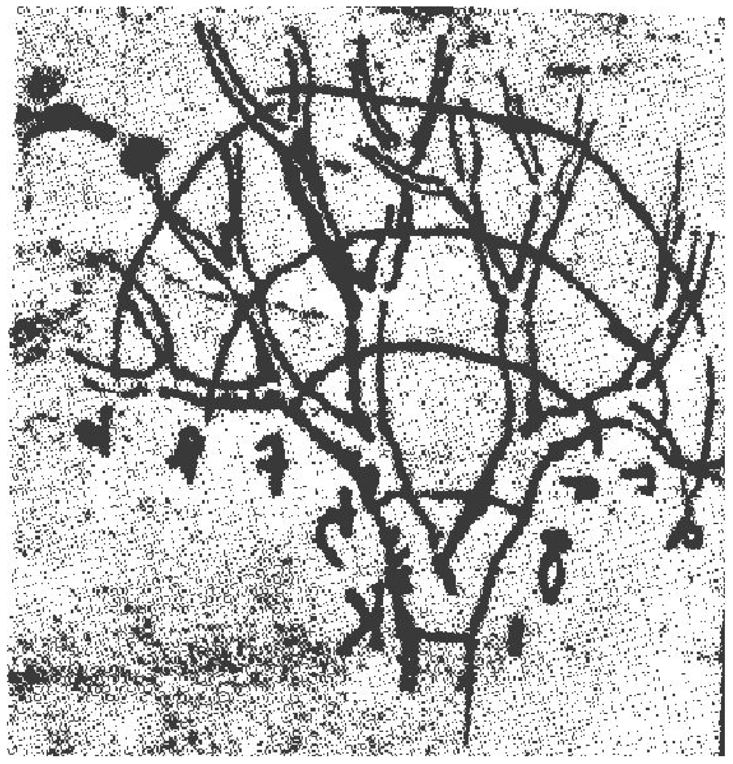
where α need not be an integer and such that if the daughter branches have equal diameters, one obtains the scaling relation $d_0=2^{1/\alpha }{d}_1$. The 500 year old scaling relation of da Vinci supplies the phenomenological mechanism necessary for AR to emerge in a number of contexts. In Figure 2 is da Vinci’s sketch of the branching structure that he used to argue for the scaling manifested by Equation (6). He applied his arguments freely to all phenomena sharing this branching behavior, including river networks.

2.2.1. Hydrology

One of the first hydrologic ARs has to do with the drainage basins of rivers. Hack [70] developed an empirical relation between the mainstream length of a river network (Y) and the drainage basin area at the closure of the river (X). In Hack’s AR, $b=\mathit{h}$ is the Hack exponent with the typical empirical value $h\approx 0.57$. He gratuitously asserted that river networks are not self-similar.

Mandelbrot [14] relates Hack’s exponent to the fractal dimension of the river network and presents a then novel interpretation of Hack’s AR. Feder [71] observed that defining a fractal dimension for river networks was obscure and required further study. A modern version of this discussion in terms of hydrologic allometry is given by Rinaldo et al. [72], who point out that optimal channel networks yield $h=0.57\pm 0.02$, suggesting that feasible optimality [73] implies Hack’s law. Another viable model is given by Sagar and Tein [74] that is geomorphology realistic, giving rise to general ARs in terms of river basin areas, as well as parallel and perpendicular channel lengths.

Figure 2. A sketch of a tree from Leonardo da Vinci’s Notebooks, PL. XXVII [69]. Note that da Vinci was relating the branches of equal generation number to also make his association with flowing streams.

Figure 2. A sketch of a tree from Leonardo da Vinci’s Notebooks, PL. XXVII [69]. Note that da Vinci was relating the branches of equal generation number to also make his association with flowing streams.

Maritan et al. [75] consider an analogy with the metabolic AR assuming a relation between parameters $\alpha =1/b$, such that $\alpha =1+h$, with the limiting values $\alpha =3/2$ and $h=1/2$, in the case of geometric self-similarity. The ensemble average of Hack’s exponents from different basins extend over 11 orders of magnitude and is indistinguishable from $h=1/2$ [76]. Maritan et al. [75] conclude that, like the interspecies metabolic rate, the slope of the intraspecies h’s are washed out in the ensemble average, resulting in the average value $h=1/2$.

2.2.2. Geology

Another empirical regularity observed in the topology of river networks is Horton’s law of river numbers [77]. Brown et al. [78] summarize the variations of flows, velocities, depths, widths and slopes in the form of an AR, where Y is the hydraulic-geometric variable and X is stream discharge and is related to the area of the discharge basin. The bifurcation parameter is the constant ratio between successive numbers of river networks, known as Horton’s law of stream numbers, and has an empirical value between 4.1 and 4.7 in natural river networks [79,80], in contrast to the random model that predicts a value of four for this ratio.

Dodds and Rothman [81] point out that universality arises when the qualitative character of a network is sufficient to quantify its essential features, such as the exponents that characterize scaling laws. They go on to say that scaling and universality have found application in the geometry of river networks and the statistical structure of topography within geomorphology. They maintain that the source of scaling in river networks and whether or not such scaling belongs to a single universality class are not yet known. They do provide a critical analysis of Hack’s law; see, also, Rodriguez-Iturbe and Rinaldo [82].

2.3. Natural History

Natural history embraces the study, description and classification of the growth and development of natural phenomena. The focus of investigation includes such important contemporary areas as ecology and paleontology, parts of which rely heavily on allometry and scaling.

2.3.1. Ecology

Ecology is the scientific study of the distribution, abundance and relations of organisms and their interactions with the environment. Such living networks include both plant and animal populations and communities, along with the network of relations among organisms of different scales of organization. Woodward et al. [83], along with many others, point out that the largest metazoans, for example, whales (${10}^8$ grams) and giant sequoias, weigh over 21 orders of magnitude more than the smallest microbes (${10}^{-13}$ grams) [35,84]. They go on to stress the considerable variation in body mass among members of the same food web.

The significance of body size has been systematically studied in ecology [84,85,86,87]. Identifying Y with species abundance and X with TBM, there is, in fact, an AR between the species at the base of a food web and the largest predator at the top [84]. We note that species-area power functions have a vital history in ecology [88,89], even though the domain of sizes over which the power law appears valid is controversial [90,91].

Brown et al. [78] discuss the universality of the documented ARs in plants, animals and microbes; to terrestrial, marine and freshwater habitats; and to human-dominated, as well as ‘natural’ ecosystems. They emphasize that the observed self-similarity is a consequence of a few basic physical, biological and mathematical principles; one of the most fundamental being the extreme variability of the data. The variety of distributions of allometry coefficients and exponents have been discussed both phenomenologically and theoretically by West and West [52].

2.3.2. Acoustic Allometry

Elephants trumpet, mice squeak and birds chirp due to scaling. Fitch [92] discusses the relationship between an organism’s body size and acoustic characterization of its vocalization under the rubric of acoustic allometry. Data indicate an AR between palate length (the skeletal proxy for vocal tract length) and body mass for a variety of mammalian species. He shows that the interspecies allometry exponent attains the geometric value of three in the regression of skull length and body mass, whereas the intraspecies allometry exponent varies a great deal. The significant variability in the intraspecies allometry exponent suggests taxon-specific factors influencing the AR [93,94].

Fitch [92] gives the parsimonious interpretation that the variability in the intraspecies allometry exponent could be the result of each species adopting allometric scaling during growth, as postulated by Huxley, with a different proportionality factor for each species. On the other hand, the interspecies allometry exponent could result from the common geometric constraints across species, due to the wide range of body sizes. He concludes that the AR between vocal tract dimensions and body size could provide accurate information about a vocalizer’s size in many mammals.

2.3.3. Paleontology

Pilbeam and Gould [95] provide reasons as to why body size plays such a significant role in biological macroevolution. The first is the statistical generalization known as Cope’s Law [96], which states that the body size of a species is an indication of how long it has survived on geological time scales. A second reason is Galileo’s observation [97] that large organisms must change shape in order to function in the same way as do their smaller prototypes.

One quantitative measure of evolution is the development of the brain in mammals at various stages of evolution. Jerison [98] showed that the brain-body AR is satisfied by mammals with an exponent that is statistically indistinguishable from 2/3. He suggested that the allometry coefficient may be an appropriate measure of brain evolution in mammals as a class.

White and Gould [99] emphasized in their review that the meaning of the allometry coefficient was unclear. Reiss [2] noted that if brain mass is regressed on TBM across individuals in a species, the slopes are shallower than those of regressions calculated across mean values for different species within a single family (genus). This argument had also been presented by Gould [100], who emphasized the importance of the allometry coefficient in the geometric similarity of allometric growth. This interpretation of the allometry coefficient was at odds with the majority of the scientific community at the time, who believed the allometry coefficient to be independent of body size. This latter view has been contradicted by contemporary data analysis [48,52].

Allometry has been used by Alberch et al. [101] as the first step in creating a unifying theory in developmental biology and evolutionary ecology in their study of morphological evolution. They demonstrate how their proposed formalism relates changes in size and shape during ontogeny and phylogeny.

Eldredge and Gould [102] argued that punctuated change dominates the history of life and that relatively rapid episodes of speciation constitute biological macroevolution. The intermittency of speciation in time has been explained by one group as punctuated equilibria [103] and has been indirectly related to fractal statistics by identifying it as a self-organized critical phenomenon [104]. In the self-organized criticality model of speciation, Bak and Boettcher [105] associate an avalanche of activity with exceeding a threshold and the distribution of returns to the threshold with a “devil’s staircase” having a distribution of steps of stasis of lengths given by the inverse power law pdf with power law index $\gamma =1.75$.

Calder [8] points out that size and time seem to be the principle characteristics of life history and ecology. West and West [106] use the time intermittency in punctuated equilibria to suggest a relation between allometry and macroevolution.

2.4. Sociology

In the allometry context, the aspect of sociology of interest are the patterns that emerge in the data that depend on the size of the social group. In large urban centers, size dependencies are found in a city’s physical structure [107], as well as in the city’s functionality, such as in the behavior of people [108]. Among the most compelling aspects of urban life, for example, income level and innovation are shown to be allometry phenomena.

2.4.1. Effect of Crowding

Farr’s law [109] is an example of the change in ARs in the transition from organismic to environmental allometry. Farr collected data from a variety of asylums in 1830s England [110] on the number of patients committed to institutions because of their mental condition and on their mortality. From these data, he was able to summarize the ”evil effect of crowding” into an AR between mortality rate Y and population density X [111]. The measure of size used in the metabolic AR, the TBM, is replaced with a measure of community structure, the population density. The ARs that capture life histories in ecology and sociology are often expressed in terms of the numbers of animals and areas in addition to TBM.

2.4.2. Urban Allometry

Batty et al. [112] examine urban spatial structure in large cities through the distribution of buildings in terms of their volume, height and area, while maintaining that there is no well worked out theory of urban allometry. As they point out, the allometry hypothesis suggests the existence of critical ratios between geometric attributes that are fixed by the functioning elements, just as in living organisms. An example they use is the dependence of natural light on the surface area of a building, so that to maintain a given ratio of natural light to building volume, the shape of the building must change with increasing size. Consequently, the volume is not given by the surface area raised to the 3/2 power, but is found empirically to have an allometry index $b\approx 1.3$. They interpret this to mean that the volume does not increase as rapidly with increasing surface area as it would for strict geometric scaling or strict rationality on the part of the builder. A number of such ARs are found between the volume, area, height and perimeter of buildings, indicating the strong influence of allometry on human design.

2.4.3. Health, Wealth and Innovation

Cities have at all times and in all places throughout history produced extremes in human activity, generating creativity, wealth, as well as crime. The allometry relation for wealth and innovation in urban centers is concave, with an allometry exponent for the population greater than one, whereas the ARs accounting for infrastructure are convex with $b<1$ [113]. The convex urban ARs share the economy of scale that is enjoyed by biological networks, since $Y/X1/X^{1-b}$ decreases with the network size, and as pointed out by Bettencourt et al. [113], this economy of scale facilitates the optimized delivery of social services, such as healthcare and education. They go on to contrast the convex with the concave urban ARs that focus on the growth of occupations oriented toward innovation and wealth creation. Of particular interest is their discussion of the scaling of rates of resource consumption with city size in direct correspondence to physiologic time. They [113] emphasize the concave situation for processes driven by innovation and wealth creation having $b>1$, manifest at an increasing pace, of urban life within larger cities [108], which they [113] quantitatively confirm for urban crime rates, the spread of infectious diseases and pedestrian walking.

3. Fractional Calculus

A dynamic fractal processes is rich in interconnected scales with no one scale dominating. It has been known since Weierstrass constructed the first fractal function in 1872 that such functions are continuous everywhere, but are no where differentiable. Consequently, such functions are not the solutions to traditional equations of motion with integer-order derivatives, and therefore, the phenomena they describe are not simple mechanical processes. Thus, information in fractal phenomena is coupled across multiple scales, as, for example, observed in the architecture of the mammalian lung [114,115,116] and in cities [107]; manifest in the long-range correlations in human gait [117,118] and the extinction of biological species [103]; measured in the human cardiovascular network [119] and in a number of other contexts [13]. The geometric interpretation of fractals is also given in the fractal nutrient model of AR [11]. Thus, we have both a deterministic and statistical application of fractals to the understanding of multi-scaled phenomena that manifest allometry patterns.

Here, we focus on the statistical nature of allometry and emphasize that allometry is strictly a relation between average quantities. This immediately brings to the forefront one of the major problems in constructing a theoretical understanding of the origins of allometry. Simply put, the measure of size X is a random variable as is the functionality, Y, and from the Jensen inequality [120], we have for a nonlinear function $Y=F\left(X\right)$:

$$〈F\left(X\right)〉\ne F\left(〈X〉\right)$$

(7)

where the brackets denote an ensemble average. Consequently, the empirical AR:

$$〈Y〉=a{〈X〉}^b$$

(8)

cannot be realized by directly averaging the schematic AR given by Equation (2) over data, since $F\left(X\right)=X^b$ is not linear for $b\ne 1$. West and West [33] sketch out the beginnings of a theory to explain how the allometry relations could originate from the scaling of the underlying statistical fluctuations.

In this section, we introduce the dynamics of observables in allometry phenomena and examine pdfs that can produce the AR given by Equation (8). There are two major techniques available in statistical physics for modeling stochastic phenomena: the first method uses the stochastic dynamic Langevin equation constructed by introducing uncertainty through a random force in the equations of motion; the second approach is based on the phase space evolution for the pdf using the Fokker–Planck equation (FPE). The conditions under which these two methods converge have been shown in a number of places [7]. One way to apply these techniques to allometry requires extending both the Langevin equation and the FPE using the fractional calculus. Herein, we explore the extension of the evolution of the pdf to fractional differential equations using the method of subordination.

3.1. Subordination

A simple stochastic process is that of Poisson in which the probability, $P\left(\tau \right)$, of an event occurring per unit time is ${\lambda }_0.$ The rate equation:

$$\frac{dP\left(\tau \right)}{d\tau }=-{\lambda }_{0}P\left(\tau \right)$$

(9)

has an exponential solution for the probability of an event occurring in a time interval $(0,\tau ).$ This is the kind of simplified dynamics Huxley adopted for the description of the differential growth of different parts of an organism. To generalize this description, we introduce the notion of subordination. This notion implies the existence of two ideas of time, as explained by Svenkeson et al. [121]. One is the operational time, τ, which is the internal time of a single individual, with an individual generating the ordinary dynamics of a non-fractional system, such as given by Equation (9). The other idea is chronological time, t: the time as measured by the clock of an external observer. The subordination procedure transforms the deterministic differential equation in operational time to a fractional differential equation in chronological time.

Note that this idea of operational time ought to be familiar. We encountered a version of it in the discussion of empirical physiologic time in which the time interval or frequency experienced by an organism is determined by the total body mass of that organism. A similar distinction is made in psychology, where the subjective time experienced by an individual in the performance of tasks is separate and distinct from the objective time of the clock on the wall [22]. Given this empirical distinction between the reality of the individual and that of the collective, mathematicians recognized the need for a time that was intrinsic to a process, whose dynamics are regular, but that appears quite complicated to an observer measuring the process from outside. Consequently, a procedure was developed to transform intrinsically regular behavior to the experimentally observed complex behavior by relating operational time to chronological time.

Svenkeson et al. [121] point out that in operational time, an individual’s behavior can appear deterministic, but to an experimenter observing the individual, their temporal behavior can appear to erratically grow in time, then abruptly to freeze in different states for extended time intervals. Due to the random nature of the evolution of the individual in chronological time, the subordination process involves an ensemble average over many individuals, each evolving according to its own internal clock, independently of one another. The resulting ensemble average over a large number of individuals results in an average trajectory that is fractal. We apply this reasoning to rate Equation (9).

The facilitate the discussion, we consider the discrete version of Equation (9):

$$P(n+1)=(1-{\lambda }_0\Delta \tau )P\left(n\right)$$

(10)

in the notation $P\left(n\right)=P\left(n\Delta \tau \right)$, where the time has been partitioned into discrete intervals. The solution to this discrete equation:

$$P\left(n\right)={(1-{\lambda }_0\Delta \tau )}^{n}P\left(0\right)$$

(11)

is an exponential, in the limit ${\lambda }_0\Delta \tau <<1$, such that $n\Delta \tau$ becomes continuous time. However, when the simple process is influenced by the environment, the limit of the discrete solution is no longer an exponential. Adopting the subordination interpretation, we define the discrete index, n, as an operational time that is stochastically connected to the chronological time, t, in which the global behavior is observed. We assume that the chronological time lies in the interval $(n-1)\Delta \tau \le t\le n\Delta \tau$, and consequently, the equation for the average dynamics of the probability is given by [122]:

$$〈P\left(t\right)〉=\underset{n=1}{\sum ^{\infty }}\stackrel{t}{\underset{0}{\int }}{G}_n\left(t,t^{\prime }\right)P\left(n\right)d{t}^{\prime }$$

(12)

The physical meaning of Equation (12) is determined by considering each tick of the internal clock, n, as measured in experimental time, to be an event. Since the observation is made in experimental time, the time intervals between events define a set of independent identically distributed random variables. The integral in Equation (12) is then built up according to renewal theory [123]. After the n-th event, it changes from state $P(n-1)$ to $P\left(n\right)$, where it remains until the action of the next event. The sum over n takes into account the possibility that any number of events could have occurred prior to an observation at experimental time t, and $G_n\left(t,t^{\prime }\right)d{t}^{\prime }$ is the probability that the last event occurs in the time interval ($t^{\prime },t^{\prime }+d{t}^{\prime }$).

We assume that the waiting times between consecutive events in Equation (12) are identically distributed independent random variables, so that the kernel is defined:

$$G_n\left(t,t^{\prime }\right)=\Psi \left(t-t^{\prime }\right){\psi }_n\left(t^{\prime }\right)$$

(13)

The probability that no event has occurred in a time, t, is given by the survival probability, $\Psi \left(t\right)$. Individual events occur statistically with a waiting-time pdf, $\psi \left(t\right)$, and taking advantage of their renewal nature, the waiting-time pdf for the n-th event in a sequence is connected to the previous event by:

$${\psi }_n\left(t\right)={\int }_0^{t}d{t}^{\prime }{\psi }_{n-1}\left(t^{\prime }\right)\psi (t-t^{\prime })$$

(14)

and ${\psi }_{{}_0}\left(t\right)=\psi \left(t\right).$ The waiting-time pdf is related to the survival probability through:

$$\psi \left(t\right)=-\frac{d}{dt}\Psi \left(t\right)$$

(15)

Here, we select the probability of no event occurring up to time t to be:

$$\Psi \left(t\right)={\left(\frac{T}{T+t}\right)}^{\alpha }$$

(16)

and consequently, the waiting-time pdf is renewal and also inverse power law.

To find an analytical expression for the behavior in experimental time, it is convenient to study the Laplace transform of Equation (12), where $\widehat{f}\left(s\right)$ denotes the Laplace transform of $f\left(t\right)$:

$$〈\widehat{P}\left(s\right)〉=\widehat{\Psi }\left(s\right)\sum _{n=0}^{\infty }P\left(n\right){\left[\widehat{\psi }\left(s\right)\right]}^n$$

(17)

and the relation ${\widehat{\psi }}_n\left(s\right)={\left[\widehat{\psi }\left(s\right)\right]}^n$ was used, due to the correlation structure of Equation (14). With the discrete time solution in operational time, Equation (11), this can be written as:

$$〈\widehat{P}\left(s\right)〉=\widehat{\Psi }\left(s\right)\sum _{n=0}^{\infty }{(1-{\lambda }_0\Delta \tau )}^{n}P\left(0\right){\left[\widehat{\psi }\left(s\right)\right]}^n$$

(18)

Performing the sum and noting the relationship given by Equation (15), we find:

$$〈\widehat{P}\left(s\right)〉=\frac{1-\widehat{\psi }\left(s\right)}{s}\frac{1}{1-(1-{\lambda }_0\Delta \tau )\widehat{\psi }\left(s\right)}P\left(0\right)$$

(19)

This can be expressed in the typical form:

$$〈\widehat{P}\left(s\right)〉=\frac{1}{s+{\lambda }_0\Delta \tau \widehat{\Phi }\left(s\right)}P\left(0\right)$$

(20)

where:

$$\widehat{\Phi }\left(s\right)=\frac{s\widehat{\psi }\left(s\right)}{1-\widehat{\psi }\left(s\right)}$$

(21)

is the Montroll–Weiss memory kernel [124].

In the asymptotic limit $s\to 0$, Equation (20) becomes:

$$〈\widehat{P}\left(s\right)〉=\frac{1}{s+\lambda s^{1-\alpha }}P\left(0\right)$$

(22)

with the parameter value:

$$\lambda =\frac{{\lambda }_0\Delta \tau }{T\Gamma \left(2-\alpha \right)}$$

Consequently, the subordination process results in ordinary rate Equation (9), through the inverse Laplace transform of Equation (22), being replaced with the fractional rate equation [121,125]:

$$D_t^{\alpha }\left[〈P\left(t\right)〉\right]-\frac{t^{-\alpha }}{\Gamma \left(1-\alpha \right)}P\left(0\right)=-\lambda 〈P\left(t\right)〉$$

(23)

where we introduce a Riemann–Liouville (RL) fractional operator. Here, we define the RL integral:

$$D_t^{-\alpha }\left[g\left(t\right)\right]\equiv \frac{1}{\Gamma \left(\alpha \right)}\stackrel{t}{\underset{0}{\int }}\frac{g\left(t^{\prime }\right)d{t}^{\prime }}{{\left(t-t^{\prime }\right)}^{1-\alpha }}$$

(24)

and the RL derivative:

$$D_t^{\alpha }\left[g\left(t\right)\right]\equiv D_t^n{D}_t^{\alpha -n}\left[g\left(t\right)\right]$$

(25)

with the operator index in the range $n-1\le \alpha \le n$ for integer n. We use the notation $D_t\left[g\left(t\right)\right]=\frac{dg\left(t\right)}{dt}.$

Note that fractional rate Equation (23) reduces to ordinary rate Equation (9) in the limit $\alpha =1$, since the gamma function diverges at zero argument. Consequently, the solution to Equation (23) must reduce to the exponential in this limit.

The solution to fractional rate equation Equation (23) was obtained by the mathematician Mittag-Leffler at the turn of the twentieth century:

$$〈P\left(t\right)〉=P\left(0\right)E_{\alpha }\left(-\lambda t^{\alpha }\right)$$

(26)

in terms of the infinite series that now bears his name:

$$E_{\alpha }\left(-\lambda t^{\alpha }\right)\equiv \underset{n=0}{\sum ^{\infty }}\frac{{\left(-\lambda t^{\alpha }\right)}^n}{\Gamma \left(n\alpha +1\right)}$$

(27)

The time dependence of the Mittag-Leffler function (MLF) is extremely interesting. At early times, the MLF has the analytic form of the stretched exponential:

$$\underset{t\to 0}{lim}{E}_{\alpha }\left(-\lambda t^{\alpha }\right)=exp\left[\frac{-\lambda t^{\alpha }}{\Gamma \left(1+\alpha \right)}\right]$$

(28)

at late times, it has the analytic form of an inverse power law:

$$\underset{t\to \infty }{lim}{E}_{\alpha }\left(-\lambda t^{\alpha }\right)=\frac{1}{\lambda \Gamma \left(1-\alpha \right)t^{\alpha }}$$

(29)

and the MLF smoothly joins these two asymptotic expressions. Consequently, the relatively benign statistics of Poisson at $\alpha =1$ become the intermittent inverse power law statistics at $0<\alpha <1.$ The complexity of the resulting statistics is captured in the power law index, much like the allometry exponent captures the complexity of the fractal structure of allometric phenomena.

3.2. Fractional Phase Space Equations

In the previous subsection, the fractional rate equation is given by Equation (23) using subordination to generalize the ordinary time derivative to the RL fractional derivative. Now, it is necessary to further extend the argument to the dynamic variable, where the probability that the dynamic variable, $Z\left(t\right)$, lies in the interval ($z,z+dz$) at time t is the phase space quantity, $P(z,t)dz$. The construction of the fractional partial differential equation for the pdf in both “space” and time and the scaling method for obtaining a solution has been presented elsewhere [33], but for the sake of completeness, I present those details here, as well. The fractional phase space equation (FPSE) with fractional derivatives in both space and time is:

$$D_t^{\alpha }\left[P(z,t)\right]-\frac{t^{-\alpha }}{\Gamma \left(1-\alpha \right)}{P}_0\left(z\right)=K_{\beta }{\partial }_{\left|z\right|}^{\beta }\left[P(z,t)\right]$$

(30)

where $D_t^{\alpha }\left[·\right]$ is the RL fractional derivative in time, ${\partial }_{\left|z\right|}^{\beta }\left[·\right]$ is the Riesz–Feller fractional derivative in one space dimension, $P_0\left(z\right)$ is the initial value of the pdf typically taken to be the delta function $\delta \left(z\right)$, and $K_{\beta }$ is a generalized diffusion coefficient. Equation (30) is sometimes called the fractional Fokker–Planck equation (FFPE) with zero potential, because it can be generalized by introducing a potential function in complete analogy with the historical Fokker–Planck equation. It is not necessary to review the fractional calculus in order to understand the solution to Equation (30) in terms of its scaling properties.

When $\alpha =1$, Equation (30) reduces to the anomalous diffusion equation [29,31,126]:

$$\frac{\partial P(z,t)}{\partial t}=K_{\beta }{\partial }_{\left|z\right|}^{\beta }\left[P(z,t)\right]$$

(31)

This equation will be useful subsequently.

The Fourier transform of the symmetric Riesz–Feller operator ${\partial }_{\left|z\right|}^{\beta }\left[·\right]$ acting on an analytic function, $\mathit{f}\left(\mathit{z}\right)$, is [29,126]:

$$FT\left\{{\partial }_{\left|z\right|}^{\beta }\left[f\left(z\right)\right],k\right\}=-{\left|k\right|}^{\beta }\tilde{f}\left(k\right)$$

(32)

where $\tilde{f}\left(k\right)$ is the Fourier transform of $f\left(z\right).$ The Laplace transform of an RL fractional time derivative $D_t^{\alpha }\left[·\right]$ acting on the analytic function, $g\left(t\right)$, is:

$$LT\left\{D_t^{\alpha }\left[g\left(t\right)\right];u\right\}=u^{\alpha }\widehat{g}\left(u\right)$$

(33)

where $\widehat{g}\left(u\right)$ is the Laplace transform of $g\left(t\right)$. Consequently, the phase space dynamics given by Equation (30) can be expressed as the Fourier–Laplace transform:

$$u^{\alpha }{P}^{*}(k,u)-u^{\alpha -1}=-K_{\beta }{\left|k\right|}^{\beta }{P}^{*}(k,u)$$

(34)

and the asterisk denotes the double transform. Therefore, the solution when $P_0\left(z\right)=\delta \left(z\right)$ in Fourier–Laplace space is:

$$P^{*}(k,u)=\frac{u^{\alpha -1}}{u^{\alpha }+K_{\beta }{\left|k\right|}^{\beta }}$$

(35)

The pdf that solves the FPSE is given by the inverse Fourier–Laplace transform of Equation (35). We note that the space-time representation of the solution to the FFPE for various combinations of α and β and potential functions are reviewed by Klafter and Metzler [29], who show how to derive Equation (30) using the continuous time random walk (CTRW) of Montroll and Weiss [124].

The inverse Laplace transform of Equation (35) yield the MLF, just as obtained in Section 3.1:

$$\tilde{P}(k,t)=E_{\alpha }\left(-K_{\beta }{\left|k\right|}^{\beta }{t}^{\alpha }\right)$$

(36)

which is the characteristic function for the process. The inverse Fourier transform of the characteristic function yields the probability density:

$$P(z,t)=\frac{1}{2\pi }\underset{-\infty }{\stackrel{\infty }{\int }}dk{e}^{-ikz}{E}_{\alpha }\left(-K_{\beta }{\left|k\right|}^{\beta }{t}^{\alpha }\right)=F{T}^{-1}\left\{E_{\alpha }\left(-K_{\beta }{\left|k\right|}^{\beta }{t}^{\alpha }\right);z\right\}$$

(37)

When $\alpha =1$, we know that the MLF reduces to an exponential, in which case, the solution is the characteristic function for the alpha-stable Lévy distribution in space with a Lévy index $0<\beta \le 2$ and a “width” that increases linearly with time:

$$P(z,t)=F{T}^{-1}\left\{Exp\left(-K_{\beta }{\left|k\right|}^{\beta }t\right);z\right\}$$

(38)

The series representation for the Lévy distribution is given in a number of places [27,31,127,128].

A variety of other solutions to the FFPE have been obtained by Mainardi [129], including the inverse Fourier transform for $\beta =2$, in which case, the solution asymptotically relaxes as the inverse power law $t^{-\alpha /2}$.

3.2.1. Statistics of Allometry Parameters

As an exemplar of the statistics of the network size, consider the growth of the average TBM across species, in which case the “space” variable is the total body mass. We assume the FFPE for the pdf to be given by:

$$\frac{\partial P(m,t)}{\partial t}=\frac{\partial }{\partial m}\left[\lambda mP(m,t)\right]+K_{\beta }{\partial }_{\left|m\right|}^{\beta }\left[P(m,t)\right]$$

(39)

where the phase space variable is $m=〈M_i〉=〈X〉$, and the discrete index for species i is suppressed for notational convenience. The Fourier transform of this equation, with $\tilde{P}(k,t)$ the Fourier transform of $P(m,t)$, yields the equation for the characteristic function:

$$\frac{\partial \tilde{P}(k,t)}{\partial t}+\lambda k\frac{\partial \tilde{P}(k,t)}{\partial k}=-K_{\beta }{\left|k\right|}^{\beta }\tilde{P}(k,t)$$

whose solution is [126]:

$$\tilde{P}(k,t)=exp\left[-\frac{K_{\beta }}{\lambda \beta }(1-e^{-\lambda \beta t}){\left|k\right|}^{\beta }\right]$$

(40)

Equation (40) is the characteristic function for a Lévy distribution with Lévy index $\beta <2.$ Note that at early times $\lambda \beta >>1/t$, the inverse Fourier transform of Equation (40) is given by Equation (38).

The asymptotic form of the pdf, obtained from the inverse Fourier transform of Equation (40), is therefore given by the inverse power law, that is, the Pareto distribution for the average TBM:

$$\underset{t\to \infty }{lim}P(〈M_i〉,t)\propto \frac{1}{{〈M_i〉}^{\beta }}$$

(41)

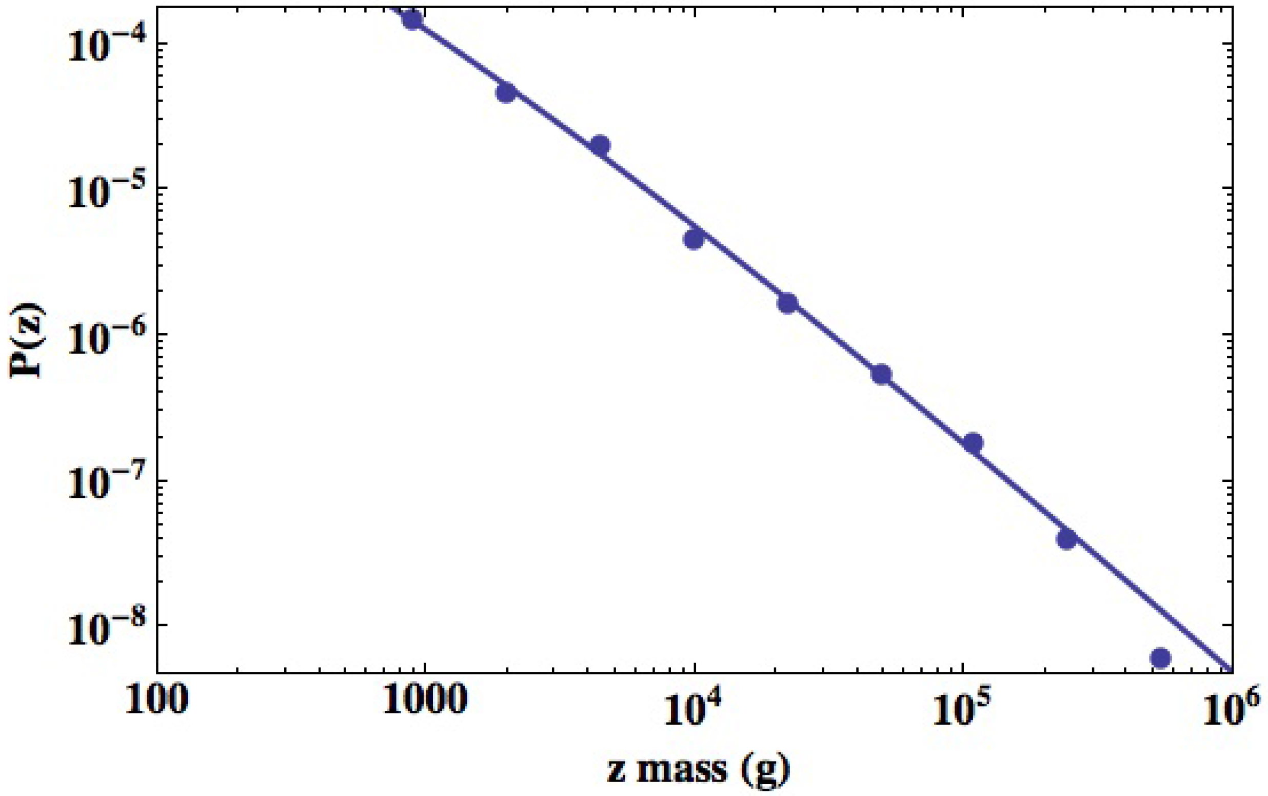
West and West [52] fit the power law index in the steady-state TBM pdf to a data set of mammalian species tabulated by Heusner [49] and depict the pdf in Figure 3. They constructed a histogram of the interspecies TBM for the 391 mammalian species from these data by partitioning the mass axis into intervals of 20 gm and counting the number of species within each of the intervals. The vertical axis is the relative number of species as a function of TBM. The figure depicts the fit to the logarithmic histogram data points indicated by dots starting at a TBM of 1.1 kg. An inverse power law would be a straight line with a negative slope on this log-log graph. Fitting the power law index from the steady-state TBM pdf to the value $\beta =1.67$ yields the solid curve in the figure, which fits the data extremely well. The curve is quite clearly an inverse power law in the interspecies TBM. This coarse-grained description of the interspecies mass statistics indicates great variability in the TBM, which is indeed the case. Moreover, since $\beta <2$, the variance of the interspecies TBM diverges or more properly increases without bound with increasing TBM.

Figure 3. The average total body mass (TBM) data for the 391 mammalian species tabulated by Heusner [49] are used to construct a histogram. The mass interval is divided into twenty equally spaced intervals on a logarithm scale and the number of species within each interval counted. The quality of the fit using the inverse power law is measured by the correlation function to be $r^2=0.998$ (From West and West [52] with permission).

Figure 3. The average total body mass (TBM) data for the 391 mammalian species tabulated by Heusner [49] are used to construct a histogram. The mass interval is divided into twenty equally spaced intervals on a logarithm scale and the number of species within each interval counted. The quality of the fit using the inverse power law is measured by the correlation function to be $r^2=0.998$ (From West and West [52] with permission).

This inverse power law in the average TBM implies a clustering of the fluctuations in mass, with bursts in the number of species near a given mass interspersed with gaps of various lengths in the mass spectrum. However, on closer inspection of these bursts of speciation, there is seen to be contained within each burst a number of smaller bursts intermittently spaced with gaps in the number of species. This intermittent bursting is characteristic of inverse power law statistics [15].

3.2.2. Urban Variability

Bettencourt et al. [130] in their study of urban scaling constructed the metric:

$${\eta }_i=ln\left[\frac{Y_i}{a{X}_i^b}\right]$$

(42)

which they called the Scale-Adjusted Metropolitan Indicators (SAMIs). They used $Y_i$ as the observed value of the measure of innovation, wealth or crime for each city, i, with population $X_i$. They found that a Laplace distribution provides an excellent fit to the normalized SAMI histogram for the statistical residuals, ${\eta }_i$, across different cities. However, they made the assumption that the allometry exponent is approximately universal.

Quite independently and contemporaneously, an analogous measure was devised by West and West [52] for the relative variation in the allometry parameters. They argued that since there are independent fluctuations in X and Y, these result in what Warton et al. [131] call equation error; also known as natural variability, natural variation and intrinsic scatter. Considering that ARs are not predictive, but instead, summarize vast amounts of data [132], this natural variability was interpreted as fluctuations in the modeling allometry parameters ($a,b$). Denoting the fitted values of the random parameters as $\overline{a}$ and $\overline{b}$, if the fluctuations are assumed to be contained in the allometry coefficient, West and West [52] define the residual in the allometry coefficient:

$${\eta }_i=ln\left[\frac{〈Y_i〉}{\overline{a}{〈X_i〉}^{\overline{b}}}\right]$$

(43)

The numerator and denominator in Equation (43) are measured independently, and in the case they were investigating, $〈Y_i〉$ is the average BMR and $〈X_i〉$ is the average TBM. The statistics of the normalized allometry coefficient, $e^{{\eta }_i}$, were determined by least squares fitting to the data to be given by a Pareto distribution. On the other hand, when the fluctuations are assumed to be constrained in the allometry exponent, they define the residual:

$${\eta }_i=\frac{ln\left(〈Y_i〉/\overline{a}\right)}{ln〈X_i〉}-\overline{b}$$

(44)

In their analysis, the allometry coefficient and exponent were held fixed, so that the parametric fluctuations fitted by a histogram gave the best fit to be that of a Laplace distribution centered on the fitted value of the allometry exponent. This latter result is completely consistent with that of Bettencourt et al. [130].

Both research groups reach the conclusion that the Laplace distributions for the statistics of the allometry exponent imply the inverse power law pdf in the size of the network. This overlap of interpretation was reached in spite of the fact that in one case, the data consisted of independent measures of BMR and TBM, which is a convex AR, and the other was on independent measurements of city economic quantities and populations in a given year, which is a concave AR. The convergence of conclusions reached in these two studies suggests the necessity of statistical measures being foundational for understanding allometry in general, as had been argued previously [15].

3.2.3. Scaling Solution

Uchaikin [133] directly inverse transformed Equation (35) for arbitrary α and β; but that level of mathematical detail is not necessary for the present analysis. For our present purposes, the desired insight is provided by directly utilizing the scaling properties of Equation (36) by considering the solution in the form of the inverse Fourier transform:

$$P(z,t)=F{T}^{-1}\left\{E_{\alpha }\left(-K_{\beta }{\left|k\right|}^{\beta }{t}^{\alpha }\right),z\right\}$$

(45)

The series expansion for the MLF allows one to write for the scaling:

$$P(Az,Bt)=\underset{n=0}{\sum ^{\infty }}\frac{{\left(-K_{\beta }{B}^{\alpha }{t}^{\alpha }\right)}^n}{\Gamma \left(n\alpha +1\right)}·\frac{\Gamma \left(n\beta +1\right)}{{\left|Az\right|}^{n\beta +1}}$$

where the second factor in the summation is the result of applying the Tauberian Theorem to the inverse Fourier transform of ${\left|k\right|}^{n\beta }$. A scaling equation emerges when the parameters satisfy the equality $A=B^{\alpha /\beta }$, resulting in:

$$P(B^{\alpha /\beta }z,Bt)=\frac{1}{B^{\alpha /\beta }}P(z,t)$$

If we now select the time parameter to be $B=1/t$, we can write:

$$P(z,t)=\frac{1}{t^{\alpha /\beta }}P\left(\frac{1}{t^{\alpha /\beta }}z,1\right)$$

(46)

Finally, the pdf that solves the FPSE in terms of the similarity variable, $z/t^{{\mu }_z}$, satisfies the scaling equation:

$$P(z,t)=\frac{1}{t^{{\mu }_z}}{F}_z\left(\frac{z}{t^{{\mu }_z}}\right)\text{and}{\mu }_z=\alpha /\beta$$

(47)

The function $F_z\left(·\right)$ in Equation (47) is left unspecified, but it is analytic in the similarity variable, $z/t^{{\mu }_z}$. As mentioned in the Introduction, a standard diffusion process, $Z\left(t\right)$, is the displacement of a diffusing particle from its initial position at time t, and for vanishing small dissipation, the scaling parameter is ${\mu }_z=1/2$ and the functional form of $F_z(·)$ is a Gauss distribution. However, for general complex phenomena, there is a broad class of distributions for which the functional form of $F_z(·)$ is not Gaussian and the scaling index ${\mu }_z\ne 1/2$. For example, the α-stable Lévy process [25,26,126,127] scales in this way and the Lévy index is in the range $0<\alpha \le 2$, with the equality holding for the Gauss distribution; the scaling index is related to the Lévy index by ${\mu }_z=1/\alpha$.

3.2.4. Allometry Relations

Of course, the stochastic variables of interest here are not necessarily space and time; they are the measures of functionality and the size of the allometry phenomena being investigated. Banavar et al. [134] used scaling theory in which $\mathit{z}$ is interpreted as the TBM, population abundance or both, and t is the region of area over which the population roams, and they obtain an expression similar in form to Equation (47). A sequence of four additional hypotheses establish a framework for the analysis of diverse empirical macroecological laws. The fractional calculus approach leading to Equation (47) is less ambitious than the scaling theory of Banavar et al. [134], but has the virtue of being able to systematically study the influence of the environment on the process of interest through the inclusion of an external force, as we did in the case of the TBM in Equation (39).

Let us now replace the space and time discussion of the previous sections with the variables of interest in an allometry context. We identify the function variable $y=Y$ with z, the average measure of size $x=〈X〉$ with t and the exponent, ${\mu }_z$, with b. In this way, the scaling pdf can be written in terms of phase space variables as:

$$P(y,x)=\frac{1}{x^b}{F}_x\left(\frac{y}{x^b}\right)$$

(48)

for a generic allometry process. The average functionality of interest is therefore given by:

$$〈Y〉=\int yP(y,x)dy=a{〈X〉}^b$$

in agreement with Equation (8). The allometry coefficient is given as the average similarity variable $q=y/x^b$:

$$a=\int q{F}_x\left(q\right)dq$$

(49)

therefore, the scaling properties of the pdf solution to the fractional phase space equation entails allometry.

Here, we noted that the allometry coefficient is determined by Equation (49), the average similarity variable. It probably does not need emphasis, but the scaling variable is precisely the quantity that was defined by the SAMI measure in Equation (42), and its average is here shown to determine the level of the allometry relation. The allometry exponent is a different matter; it is given by the ratio of the scaling index, α, for the fractional derivative in time and the scaling index, β, for the fractional derivative in “space”. Consequently, the ratio denotes a balance between the memory of the underlying process, with $\alpha =1$ indicating no memory, and the nonlocal nature in the phase space of the variate, with $\beta =2$ indicating a homogeneous local process, such as obtained in classical diffusion. However, the allometry relation only yields their ratio, being as it is a relationship between averages. In order to untangle their separate contributions to allometry, requires a more detailed statistical study.

4. Discussion and Conclusions

One reason for the introduction of the fractional calculus into the discussion of allometry relations was the fact that “time” for the lumbering elephant is not the same as that for a humming bird. As West and West [61] point out, the “time” shared by the two species is the same when referenced to a physical clock, but is not the same when referenced to their individual physiology. This realization led us to introduce the mathematics of subordination to transform a normal rate process into a fractional rate process and to recast the allometry scaling arguments into the formalism of the fractional calculus. We also took cognizance of the fact that allometry scaling is not a property of the dynamic variables, which are stochastic, but is rather a property of the probability density functions. Consequently, the ordinary probability calculus had to be replaced with the fractional probability calculus in which the equations of motion for the probability density function have one or more fractional derivatives.

The dynamics of allometry phenomena have been treated as interdependent dynamical statistical allometry variables in terms of the fractional probability calculus. A fractional Fokker–Planck equation with the network size as the dependent variable (in this case, the network size is the total body mass) was shown to have a steady-state solution that is a Lévy distribution. The asymptotic form of the Lévy distribution is the inverse power law, which is shown to fit the distribution of TBM across species. It should be noted that this recognition of the asymptotic inverse power law behavior of the TBM is fairly recent [52].

From this new fractional probability calculus perspective, a number of results were derived that had previously been restricted to the contexts in which they were originally developed. For example, the statistical variability of the allometry exponent around its average value was found to be described by a Laplace distribution for the metabolic AR [52], as well as for a number of urban ARs [130] by completely different arguments. Here, it was demonstrated that they both are the consequence of the same statistical scaling. These results suggest the universality of using the probability calculus generalized to fractional form to capture the underlying complexity of allometry phenomena regardless of the source of the dynamics.

The representation of allometry phenomena in terms of the joint pdf of the system size and functionality has been shown to be very useful. The scaling property of the pdf solution to the fractional phase space equations was shown to entail an allometry relation between the average functionality and the average measure of the network size. This AR could not be rigorously derived previously, due to the Jensen inequality. Consequently, one may cautiously observe that the origin of allometry relations lies with the scaling behavior of the underlying statistical processes.

Allometry can now be interpreted to be a consequence of the the fact that the two measures of the complex phenomenon, function and size are statistically tied together as a ratio, independently of how they fluctuate separately. A consequence of there being a ratio is that the separate fluctuations cannot be disentangled. The allometry exponent, b, is the ratio of the scaling indices, α and β, not unlike the ratio of growth indices in the Huxley “derivation” of the allometry relation.

Note that the present analysis does not invalidate the mechanism-specific arguments that various investigators have ingeniously constructed to explain allometry relations in particular contexts. The fractional probability calculus explanation of AR is compatible with the fractal nutrient network model of West et al. [35]; it is consistent with the renormalization scaling of Banavar et al. [134]; it does not contradict the data analysis of Glazier [48] nor does it conflict with Bejan’s constructal law [50].

A purist might criticize the assertion that scaling statistics entail allometry as being phenomenologically based and, therefore, is not a ‘real’ explanation of the origin of allometry. My only defense is to point to the utility of thermodynamics and observe that it too is mere phenomenology that lacks such a ‘fundamental’ explanation.

References

- Gould, S.J. Allometry and size in ontogeny and phylogeny. Biol. Rev. Cam. Philos. Soc. 1966, 41, 587–640. [Google Scholar] [CrossRef]
- Reiss, M.J. The Allometry of Growth and Reproduction; Cambridge University Press: Cambridge, UK, 1989. [Google Scholar]
- Thompson, D.W. On Growth and Form, The Complete Revised Edition; Dover: New York, NY, USA, 1992. [Google Scholar]
- Huxley, J.S. Problems of Relative Growth; Dial Press: New York, NY, USA, 1931. [Google Scholar]
- Lorenz, E.N. The Essence of Chaos; University of Washington Press: Seattle, WA, USA, 1993. [Google Scholar]
- Ott, E. Chaos in Dynamical Systems; Cambridge University Press: New York, NY, USA, 1993. [Google Scholar]
- Lindenberg, K.; West, B.J. The Nonequilibrium Statistical Mechanics of Open and Closed Systems; VCH: New York, NY, USA, 1990. [Google Scholar]
- Calder, W.W., III. Size, Function and Life History; Harvard University Press: Cambridge, MA, USA, 1984. [Google Scholar]
- Schmidt-Nielsen, K. Scaling, Why is Animal Size so Important? Cambridge University Press: Cambridge, UK, 1984. [Google Scholar]
- Banavar, J.R.; Damuth, J.; Maritan, A.; Rinaldo, A. Allometric cascades. Nature 2003, 421, 713–714. [Google Scholar] [CrossRef] [PubMed]
- West, G.B.; Brown, J.H.; Enquist, B.J. A general model for the origin of allometric scaling laws in biology. Science 1997, 276, 122–124. [Google Scholar] [CrossRef] [PubMed]
- Weissman, M.B. 1/f noise and other slow, nonexponential kinetics in condensed matter. Rev. Mod. Phys. 1988, 60, 537–571. [Google Scholar] [CrossRef]
- West, B.J.; Geneston, E.L.; Grigolini, P. Maximizing information exchange between complex networks. Phys. Rept. 2008, 468, 1–99. [Google Scholar] [CrossRef]
- Mandelbrot, B.B. Fractals, Form and Chance; W.H. Freeman: San Francisco, CA, USA, 1977. [Google Scholar]
- West, D.; West, B.J. On allometry relations. Int. J. Mod. Phys. 2012, 26, 1230013–1230014. [Google Scholar] [CrossRef]
- Mandelbrot, B.B. Self-Affine Fractal Sets. In Fractals in Physics; Pietronero, L., Tosatti, E., Eds.; North-Holland: Amsterdam, The Netherlands, 1986; pp. 3–28. [Google Scholar]
- Mandelbrot, B.B. Fractals and Scaling in Finance; Springer: New York, NY, USA, 1997. [Google Scholar]
- Mantegna, R.N.; Stanley, H.E. Econophysics; Cambridge University Press: New York, NY, USA, 2000. [Google Scholar]
- Allegrini, P.; Paadissi, P.; Menicci, D.; Gemignani, A. Fractal complexity in spontaneous EEG metastable-state transitions: New vistas on integrated neural dynamics. Front. Physiol. 2010, 1. [Google Scholar] [CrossRef] [PubMed]
- Werner, G. Frctals in the nervous system: Conceptual implications for theoretical neuroscience. Front. Physiol. 2010, 1. [Google Scholar] [CrossRef]
- Turcotte, D.L. Fractals and Chaos in Geology and Geophysics; Cambridge University Press: Cambridge, UK, 1992. [Google Scholar]
- West, B.J. Fractal physiology and the fractional calculus: A perspective. Front. Physiol. 2010, 1. [Google Scholar] [CrossRef]
- West, B.J.; Grigolini, P. Complex Webs: Anticipating the Improbable; Cambridge University Press: Cambridge, UK, 2011. [Google Scholar]
- Beran, J. Statistics of Long-Memory Processes. In Monographs on Statistics and Applied Probability; Chapman & Hall: New York, NY, USA, 1994; Volume 61. [Google Scholar]
- Samorodnitsky, G.; Taqqu, M.S. Stable Non-Gaussian Random Processes; Chapman & Hall: New York, NY, USA, 1994. [Google Scholar]
- Zolotarev, V.M. One-Dimensional Stable Distributions; Translations of Mathematical Monographs, American Mathematical Society: Providence, RI, USA, 1986; Volume 65. [Google Scholar]
- Magin, R.L. Fractional Calculus in Bioengineering; Begell House: Redding, CT, USA, 2006. [Google Scholar]
- Miller, K.S.; Ross, B. An Introduction to the Fractional Calculus and Fractional Differential Equations; John Wiley & Sons: New York, NY, USA, 1993. [Google Scholar]
- Klafter, J.; Metzler, R. The random walk’s guide to anomalous diffusion: A fractional dynamics approach. Phys. Rept. 2000, 339, 1–77. [Google Scholar] [CrossRef]
- Sokolov, I.M.; Klafter, J.; Blumen, A. Fractional kinetics. Phys. Today 2002, 55, 48–54. [Google Scholar] [CrossRef]
- West, B.J.; Bologna, M.; Grigolini, P. Physics of Fractal Operators; Springer: Berlin, Germany, 2003. [Google Scholar]
- West, B.J.; West, D. Origin of Allometry Hypothesis. In Fractal Dynamics; Recent Advances; Klafter, J., Lin, S.C., Metler, R., Eds.; World Scientific: Singapore, 2011. [Google Scholar]
- West, B.J.; West, D. Fractional Dynamics of Allometry. Frac. Calc. App. Anal. 2012, 15, 70–96. [Google Scholar] [CrossRef]
- Banavar, J.R.; Damuth, J.; Maritan, A.; Rinaldo, A. Modeling universality and scaling. Nature 2002, 420, 626–627. [Google Scholar] [CrossRef] [PubMed]
- West, G.B.; Brown, J.H.; Enquist, B.J. The fourth dimension of life: Fractal geometry and allometric scaling of organisms. Science 1999, 284, 11677–1679. [Google Scholar] [CrossRef]
- Gayon, J. History of the concept of allometry. Am. Zool. 2000, 40, 748–758. [Google Scholar] [CrossRef]
- Cuvier, G. Recherches sur les Ossemens Fossils; Chez G. Dufour et E. d’Ocagne: Paris, France, 1821. [Google Scholar]
- Snell, O. Die Abhängigkeit des Hirngewichts von dem Körpergewicht und den geistigen Fähigkeiten. Arch. Psychiatr. 1892, 23, 436–446. [Google Scholar] [CrossRef]
- Tower, D.B. Structural and functional organization of mammalian cerebral cortex the correlation of neurone density with brain size. J. Comput. Neurol. 1954, 101, 9–52. [Google Scholar]
- Changizi, M.A. Principles underlying mammalian neocortical scalling. Biol. Cybern. 2001, 84, 207–215. [Google Scholar] [CrossRef] [PubMed]
- Sarrus, R. Rapport sur un memoire adresse a L’Academie Royle de Medcine. Commissaires Robiquet et Thillarye, rapporteurs. Bull. Acad. Roy. Med. (Paris) 1838–1839, 3, 1094–1000. [Google Scholar]
- Rubner, M. Ueber den Einfluss der Körpergrösse auf Stoffund Kraftwechsel. Z. Biol. 1883, 19, 353–358. [Google Scholar]
- Kleiber, M. Body size and metabolism. Hilgarida 1932, 6, 315–353. [Google Scholar] [CrossRef]
- Brody, S. Bioenergetics and Growth; Reinhold: New York, NY, USA, 1945. [Google Scholar]
- Hemmingsen, A.M. The relation of standard (basal) energy metabolism to total fresh weight of living organisms. Rep. Steno. Mem. Hosp. (Copenhagen) 1950, 4, 1–58. [Google Scholar]
- Dodds, P.S.; Rothman, D.H.; Weitz, J.S. Re-examination of the 3/4-law of metabolism. J. Theor. Biol. 2001, 209, 9–27. [Google Scholar] [CrossRef] [PubMed]
- Glazier, D.S. Beyond the ‘3/4-power law’: Variation in the intra- and interspecific scaling of metabolic rate in animals. Biol. Rev. 2005, 80, 611–662. [Google Scholar] [CrossRef] [PubMed]
- Glazier, D.S. A unifying explanation for diverse metabolic scaling in animals and plants. Biol. Rev. 2010, 85, 111–138. [Google Scholar] [CrossRef]
- Heusner, A.A. Size and power in mammals. J. Exp. Biol. 1991, 160, 25–54. [Google Scholar] [PubMed]
- Bejan, A. The tree of convective heat streams: Its thermal insulation function and the predicted 3/4-power relation between body heat loss and body size. Int. J. Heat Mass Trans. 2001, 44, 699–704. [Google Scholar] [CrossRef]
- Glazier, D.S. The 3/4-power law is not universal: Evolution of isomeric, ontogenetic metabolic scaling in pelagoic animals. BioScience 2006, 56, 325–332. [Google Scholar] [CrossRef]
- West, D.; West, B.J. Stochastic origin of allometry. EPL 2001, 94. [Google Scholar] [CrossRef]
- Hill, A.V. The dimensions of animals and their muscular dynamics. Sci. Prog. 1950, 38, 209–230. [Google Scholar]
- Lindstedt, S.L.; Calder, W.A., III. Body size and longevity in birds. Condor 1976, 78, 91–94. [Google Scholar] [CrossRef]
- Lindstedt, S.L.; Miller, B.J.; Buskirk, S.W. Home range, time and body size in mammals. Ecology 1986, 67, 413–418. [Google Scholar] [CrossRef]
- Lindstedt, S.L.; Calder, W.A., III. Body size, physiological time, and longevity of homeothermic animals. Quart. Rev. Biol. 1981, 36, 1–16. [Google Scholar] [CrossRef]
- Ballard, F.J.; Hanson, R.W.; Kronfeld, D.S. Gluconeogenesis and lipogenesis in tissue from ruminant and nonruminant animals. Fed. Proc. 1969, 28, 218–231. [Google Scholar] [PubMed]
- Sacher, G.A. Relation of Lifespan to Brain Weight and Body Weight in Mammals. In Ciba Foundation Colloquium on Aging; Wolstenholme, G.E.W., Ed.; John Wiley and Sons: Chichester, UK, 1959; Volume 1. [Google Scholar]
- Heusner, A.A. Energy metabolism and body size: I. Is the 0.75 mass exponent of Kleiber’s equation a statistical artifact? Resp. Physiol. 1982, 4, 1–12. [Google Scholar] [CrossRef]
- Savage, V.M.; Gillooly, J.P.; Woodruff, W.H.; West, G.B.; Allen, A.P.; Enquist, B.J.; Brown, J.H. The predominance of quarter-power scaling biology. Func. Ecol. 2004, 18, 257–282. [Google Scholar] [CrossRef]
- West, D.; West, B.J. Physiologic time: A hypothesis. Phys. Life Rev. 2013, 10, 210–224. [Google Scholar] [CrossRef] [PubMed]
- Hempleman, S.C.; Kilgore, D.L.; Colby, C.; Bavis, R.W.; Powell, F.L. Spike firing allometry in avian intrapulmonary chemoreceptors: Matching neural code to body size. J. Exp. Biol. 2005, 208, 3065–3073. [Google Scholar] [CrossRef] [PubMed]
- Niklas, K.J. Plant allometry: Is there a grand unifying theory? Biol. Rev. 2004, 79, 871–889. [Google Scholar] [CrossRef] [PubMed]
- Reich, P.B.; Tjoelker, M.G.; Marchado, J.; Oleksyn, J. Universal scaling of respiratory metabolsim, size and nitrogen in plants. Nature 2006, 439, 457–461. [Google Scholar] [CrossRef]
- Enquist, B.J. Universal scaling in tree and vascular plant allometry: Towards a general quantitative theory linking plant form and function from cells to ecosystems. Tree Phys. 2002, 22, 1045–1064. [Google Scholar] [CrossRef]
- Bassett, D.S.; Greenfield, D.L.; Meyer-Lindenberg, A.; Weinberger, D.R.; Moore, S.W.; Bullmore, E.T. Efficient physical embedding of topologically complex information processing networks in brains and computer circuits. PLoS Comput. Biol. 2010, 6, 1–14. [Google Scholar] [CrossRef] [PubMed]
- Schlenska, G. Volumen und Oberflachenmessungen an Gehiren verschiedener Saugetiere im Vergleich su einem errechneien Modell. J. Hirnforsch 1974, 15, 401–408. [Google Scholar]
- Beiu, V.; Ibrahim, W. Does the brain really ouperfofrm Rent’s rule? In Proceedings of IEEE International Symposium on Circuits and Systems (ISCAS 2008), Seattle, WA, USA, 18–21 May 2008; pp. 640–643.
- Richter, J.P. The Notebooks of Leonardo da Vinci; Dover: New York, NY, USA, 1970; Volume 1, Unabridged edition of the work first published in London in 1883. [Google Scholar]
- Hack, J.T. Studies of longitudianl profiles in Virginia and Maryland. Geol. Surv. Prof. Pap. 1957, 294-B, 1–52. [Google Scholar]
- Feder, J. Fractals; Plenum: New York, NY, USA, 1988. [Google Scholar]
- Rinaldo, A.; Banavar, J.R.; Maritan, A. Trees, networks and hydrology. Water Resour. Res. 2006, 42, 1–19. [Google Scholar] [CrossRef]
- Rigon, R.; Rodriguez-Iturbe, I.; Rinaldo, A. Feasible optimality implies Hack’s law. Water Resour. Res. 1998, 32, 3367–3374. [Google Scholar] [CrossRef]
- Sagar, B.S.; Tien, T.L. Allometric power-law relationships in a Hortonian fractal digital elevation model. Geophys. Res. Lett. 2004, 31, L06501:1–L06501:4. [Google Scholar] [CrossRef]
- Maritan, A.; Rigon, R.; Banavar, J.B.; Rinaldo, A. Network allometry. Geophys. Res. Lett. 2001, 29, 1508. [Google Scholar] [CrossRef]
- Montgomery, D.R.; Dierich, W.E. Channel initiation and the problem of landscape scale. Science 1992, 255, 826–832. [Google Scholar] [CrossRef] [PubMed]
- Horton, R.E. Erosional development of streams and their drainage basins: Hydophysical approach to quantitative geomorphology. Geol. Soc. Am. Bull. 1945, 56, 275–370. [Google Scholar] [CrossRef]
- Brown, J.H.; Gupta, V.K.; Li, B.; Milne, B.T.; Restrepo, C.; West, G.B. The fractal nature of nature: Power laws, ecological complexity and biodiversity. Phil. Trans. R. Soc. Lond. B 2002, 357, 619–626. [Google Scholar] [CrossRef] [PubMed]
- Peckham, S. New results for self-similar trees with appllications to river networks. Water Resour. Res. 1995, 31, 1023–1029. [Google Scholar] [CrossRef]
- Peckham, S.D.; Gupta, V.K. A reformulation of Horton’s law for large river networks in terms of statistical self-similarity. Water Resour. Res. 1999, 35, 2763–2777. [Google Scholar] [CrossRef]
- Dodds, P.S.; Rothman, D.H. Scaling, universality and geomorphology. Ann. Rev. Earth Planet. Sci. 2000, 28, 1–41. [Google Scholar] [CrossRef]
- Rodriguez-Iturbe, I.; Rinaldo, A. Fractal River Basins. Chance and Self-organization; Cambridge University Press: Cambridge, UK, 1997. [Google Scholar]
- Woodward, G.; Ebenman, B.; Emmerson, M.; Montoya, J.M.; Olesen, J.M.; Valido, A.; Warren, P.H. Body size in ecological networks. Trends Ecol. Evol. 2005, 20, 402–409. [Google Scholar] [CrossRef] [Green Version]
- Cohen, J.E.; Jonsson, T.; Carpenter, S.R. Ecological community description using the food web, spcies abundance, and body size. Proc. Natl. Acad. Sci. USA 2003, 100, 1781–1786. [Google Scholar] [CrossRef] [PubMed]
- Brown, J.H.; Gillooly, J.F.; Allen, A.P.; Savage, V.M.; West, G.B. Toward a metabolic theory of ecology. Ecology 2004, 85, 1771–1789. [Google Scholar] [CrossRef]
- Brown, J.H.; Gillooly, J.F.; Allen, A.P.; Savage, V.M.; West, G.B. Response to forum commentary on Toward a metabolic theory of ecology. Ecology 2004, 85, 1818–1821. [Google Scholar] [CrossRef]
- Jonsson, T.; Cohen, J.E.; Carpenter, S.R. Food webs, body size and species abundance in ecological community description. Adv. Ecol. Res. 2005, 36, 1–84. [Google Scholar]
- Preston, F.W. The canonical distribution of commonness and rarity. Ecology 1962, 43, 185–215. [Google Scholar] [CrossRef]
- Willis, J.C. Age and Area; Cambridge University Press: Cambridge, UK, 1922. [Google Scholar]
- Brown, J.H. Macroecology; University of Chicago Press: Chicago, IL, USA, 1995. [Google Scholar]
- Williams, C.B. Patterns in the Balance of Nature and Related Problems in Quantitative Ecology; Academic Press: New York, NY, USA, 1964. [Google Scholar]
- Fitch, W.T. Skull dimensions in relation to body size in nonhuman mammals: The causal bases for acoustic allometry. Zoology 2000, 103, 40–58. [Google Scholar]
- Martin, R.D.; Harvey, P.H. Brain Size Allometry: Ontogeny and Phylogeny. In Size & Scaling in Primate Biology; Jungers, W.L., Ed.; Plenum Press: New York, NY, USA, 1985. [Google Scholar]
- Shea, B. Relative growth of the limbs and trunk in the African apes. Am. J. Phys. Anthopol. 1981, 56, 179–202. [Google Scholar] [CrossRef] [PubMed]
- Pilbeam, D.; Gould, S.J. Size and scaling in human evoluton. Science 1974, 186, 892–901. [Google Scholar] [CrossRef] [PubMed]
- Cope, E.D. The Primary Factors of Organic Evolution; Open Court Publishing Company: London, UK, 1896. [Google Scholar]
- Galileo, G. This is in the Dialogue of the Second Day in the Discorsi of 1638, the work Galileo wrote while under house arrest by the Inquisition. It was translated as Dialogues Concerning Two New Sciences by H. Crew and A De Salvor in 1914 and reprinted by Dover, New York, 1952.
- Jerison, H.J. Quantitative analysis of evolution of the brain in mammals. Science 1961, 133, 1012–1014. [Google Scholar] [CrossRef] [PubMed]
- White, J.F.; Gould, S.J. Interpretation of the coefficient in the allometric equation. Am. Nat. 1965, 99, 5–18. [Google Scholar] [CrossRef]
- Gould, S.J. Geometric similarity in allometric growth: A contribution to the problem of scaling in the evolution of size. Am. Nat. 1971, 105, 113–136. [Google Scholar] [CrossRef]
- Alberch, P.; Gould, S.J.; Oster, G.F.; Wake, D.B. Size and shape in ontogeny and phylogeny. Paleobiology 1979, 5, 296–317. [Google Scholar]
- Eldredge, N.; Gould, S.J. Punctuated Equilibria: An Alternative to Phyletic Gradualism. In Models in Paleobiology; Schopf, T.J.M., Ed.; Freeman, Cooper and Co.: San Francisco, CA, USA, 1972; pp. 82–115. [Google Scholar]
- Eldredge, N. Time Frames; Princeton University Press: Princeton, NJ, USA, 1985. [Google Scholar]
- Sneppen, K.; Bak, P.; Flybjerg, H.; Jensen, M.H. Evolution as a self-organized critical phenomenon. Proc. Natl. Acad. Sci. USA 1995, 92, 5209–5213. [Google Scholar] [CrossRef] [PubMed]
- Bak, P.; Boettcher, S. Self-organized criticality and punctuated equilibrium. Phys. D 1997, 107, 143–150. [Google Scholar] [CrossRef]
- West, D.; West, B.J. Are allometry and macroevolution related? Phys. A 2011, 390, 1733–1736. [Google Scholar] [CrossRef]
- Batty, M.; Longley, P. Fractal Cities; Academic Press: New York, NY, USA, 1994. [Google Scholar]
- Milgrim, S. The experience of living in cities. Science 1970, 167, 1461. [Google Scholar] [CrossRef]
- Brownlee, J. Density of death rate: Farr’s law. J. Roy. Soc. Stat. Soc. 1920, 83, 280–283. [Google Scholar] [CrossRef]
- Farr, W. A report on the mortality of lunitacs. J. Stat. (London) 1841, 9, 17–33. [Google Scholar]
- Humphreys, N.A. Vital Statistics: A Memorial Volume of Selections from the Reports and Writings of William Farr; The Sanitory Institute of Great Britian: London, UK, 1885. [Google Scholar]
- Batty, M.; Carvalho, R.; Hudson-Smith, A.; Milton, R.; Smith, D.; Steadman, P. Geometric Scaling and Allometry in Large Cities. In Proceedings of the 6th International Space Syntax Symposium, Istanbul, Turkey, 2007.
- Bettencourt, L.M.A.; Lobo, J.; Helbing, D.; Kuhnert, C.; West, G.B. Growth, innovation, scaling and the pace of life in cities. Proc. Natl. Acad. Sci. USA 2007, 104, 7301–7306. [Google Scholar] [CrossRef] [PubMed]
- Nelson, T.R.; West, B.J.; Goldberger, A.L. The fractal lung: Universal and species-related scaling patterns. Experientia 1990, 46, 251–254. [Google Scholar] [CrossRef] [PubMed]
- Weibel, E.R. Symmorphosis: On Form and Function in Shaping Life; Harvard University Press: Cambridge, MA, USA, 2000. [Google Scholar]
- West, B.J.; Barghava, V.; Goldberger, A.L. Beyond the principle of similitude: Renormaization in the bronchial tree. J. Appl. Physiol. 1986, 60, 1089–1097. [Google Scholar] [PubMed]
- Hausdorff, J.M.; Purdon, P.L.; Peng, C.-K.; Ladin, Z.; Wei, J.Y.; Goldberger, A.L. Fractal dynamics of human gait: Stability of long-range correlations. J. Appl. Physiol. 1996, 80, 1448–1457. [Google Scholar] [PubMed]
- West, B.J. The Lure of Modern Science: Fractal Thinking; Studies of Nonlinear Phenomena in Life Science; World Scientific: Singapore, 1999; Volume 3. [Google Scholar]
- Peng, C.-K.; Mistus, J.; Hausdorff, J.M.; Havlin, S.; Stanley, H.E.; Goldberger, A.L. Long-range anti-correlations and non-Gaussian behavior of the heartbeat. Phys. Rev. Lett. 1993, 70, 1343–1346. [Google Scholar] [CrossRef]
- Jensen, J.L.W.V. Sur les fonctions convexes et les inégalités entre les valeurs moyennes. Acta Math. 1906, 30, 175–193. [Google Scholar] [CrossRef]
- Svenkeson, A.; Beig, M.T.; Turalska, M.; West, B.J.; Grigolini, P. Fractional trajecories: Decorrelation verus friction. Phys. A 2013, 392, 5663–5672. [Google Scholar] [CrossRef]
- Pramukkul, P.; Svenkeson, A.; Grigolini, P.; Bologna, M.; West, B.J. Complexity and the Fractional Calculus. Adv. Math. Phys. 2013, 2013, 498789:1–498789:7. [Google Scholar] [CrossRef]
- Weiss, G.H. Aspects and Applications of the Random Walk; North-Holland: Amsterdam, The Netherlands, 1994. [Google Scholar]
- Montroll, E.W.; Weiss, G. Random walks on lattices. II. J. Math. Phys. 1965, 6, 167–181. [Google Scholar] [CrossRef]
- Sokolov, I.M.; Klafter, J. From diffusion to anomalous diffusion: A centruy after Einstein’s Brownian motion. Chaos 2005, 15, 026103–026109. [Google Scholar] [CrossRef] [PubMed]
- Seshadri, V.; West, B.J. Fractal dimensionality of Lévy processes. Proc. Natl. Acad. Sci. USA 1982, 79, 4501–4505. [Google Scholar] [CrossRef] [PubMed]
- Montroll, E.W.; West, B.J. On an Enriched Collection of Stochastic Processes. In Fluctuation Phenomena; Montroll, E.W., Lebowitz, J.L., Eds.; North-Holland: Amsterdam, The Netherlands, 1979. [Google Scholar]
- Podlubny, I. Fractional Differential Equations, Mathematics in Science and Engineering; Academic Press: San Diego, CA, USA, 1999; Volume 198. [Google Scholar]
- Mainardi, F.; Mura, A.; Pagnini, G.; Gorenflo, R. Time-fractional diffusion of distributed order. J. Vib. Control 2007, 10, 269–308. [Google Scholar] [CrossRef]
- Bettencourt, L.M.A.; Lobo, J.; Strumsky, D.; West, G.B. Urban scaling and its Deviations: Revealling the structure of wealth, innovation and crime across cities. PLoS ONE 2010, 5, e1354. [Google Scholar] [CrossRef] [PubMed]
- Warton, D.I.; Wright, I.J.; Falster, D.S.; Westoby, M. Bivariate line fitting methods for allometry. Biol. Rev. 2006, 85, 259–291. [Google Scholar] [CrossRef] [PubMed]
- White, C.R.; Cassey, P.; Blackburn, T.M. Metabolic allometry exponents are not universal. Ecology 2007, 88, 315–323. [Google Scholar] [CrossRef] [PubMed] [Green Version]
- Uchaikin, V.V. Montroll-Weiss problem, fractional diffusion equations and stable distribution. Int. J. Theor. Phys. 2000, 39, 3805–3813. [Google Scholar] [CrossRef]
- Banavar, J.R.; Damuth, J.; Maritan, A.; Rinaldo, A. Scaling in ecosystems and the linkage of macroecological laws. Phys. Rev. Lett. 2007, 98. [Google Scholar] [CrossRef]
© 2014 by the author; licensee MDPI, Basel, Switzerland. This article is an open access article distributed under the terms and conditions of the Creative Commons Attribution license (http://creativecommons.org/licenses/by/3.0/).
Share and Cite
MDPI and ACS Style
West, B.J. A Fractional Probability Calculus View of Allometry. Systems 2014, 2, 89-118. https://0-doi-org.brum.beds.ac.uk/10.3390/systems2020089
AMA Style
West BJ. A Fractional Probability Calculus View of Allometry. Systems. 2014; 2(2):89-118. https://0-doi-org.brum.beds.ac.uk/10.3390/systems2020089
Chicago/Turabian StyleWest, Bruce J. 2014. "A Fractional Probability Calculus View of Allometry" Systems 2, no. 2: 89-118. https://0-doi-org.brum.beds.ac.uk/10.3390/systems2020089