Real-Time Implementation of Green Light Optimal Speed Advisory for Electric Vehicles


Ben-Gurion University, P.O.B. 653, Beer-Sheva 8410501, Israel
*
Author to whom correspondence should be addressed.
Vehicles 2020, 2(1), 35-54; https://0-doi-org.brum.beds.ac.uk/10.3390/vehicles2010003
Submission received: 19 November 2019
/
Revised: 5 January 2020
/
Accepted: 14 January 2020
/
Published: 17 January 2020
Abstract
:Intelligent Transportation Systems (ITS), such as Green Light Optimal Speed Advisory (GLOSA) systems, can be used to reduce the energy consumption in modern vehicles. In particular, GLOSA systems provide driving strategies that can decrease both energy consumption and travel time. In this paper, we present a new method to calculate the optimal driving speeds based on traffic light data. To this end, a detailed formulation for the optimization problem is presented for a multi-segment route, based on an electric vehicle (EV) and traffic light models in an urban environment. Since this formulation results in a nonconvex optimization problem, a relaxation procedure is applied with a low calculation time. By using this procedure, a dynamic real-time speed advisory algorithm is developed. Numerical simulations showed improved performance over benchmark techniques. In particular, the proposed Dynamic-GLOSA solution’s performance was shown to be very close to that with a brute-force optimal solution but with a much shorter calculation time and has significant potential for energy saving.
1. Introduction
The global energy crisis and the growing dependency on oil lead to serious environmental consequences that threaten price stability and global economic growth [1]. Electric vehicles (EV) are becoming increasingly common, to the extent that governments encourage their use because of their high energy efficiency and zero emissions during operation [2]. However, the current capacity for battery stored electrical energy offers low energy density compared to fuel [3], which affects the maximum range can be reached without recharging the battery. Energy efficient driving is a promising way to deal with the EV range problem and the energy dependence.
Intelligent Transportation Systems (ITS) exploit advances in infrastructure-to-vehicle communication (I2V) to optimize transportation efficiency. The ongoing improvement in calculation abilities makes it possible to optimize processes in numerous fields, such as transportation and power management [4]. A proper driving strategy has great potential for reducing fuel and energy consumption [5], emission [6], and trip time [7]. ITS solutions include adaptive signal control [8,9], optimal route planning [10,11], and driving strategy advisory systems. Signal control and route planning seek to minimize idling and travel time cost functions. Driving strategy advisory systems provide velocity or acceleration recommendations that take travel time and energy consumption into account. In particular, Green Light Optimal Speed Advisory (GLOSA) systems enable significant savings in fuel consumption and idling time by using road data and traffic light schedules.
GLOSA is an advanced driver assistance system (ADAS) that advises the driver to employ a chosen speed in order to arrive at each intersection during a green light phase. The desired speed is computed according to various criteria [5,7,12,13,14,15] that are described by an objective function, which is usually based on various factors such as total energy consumption and travel time. GLOSA system algorithms use traffic signal phase and timing information, as well as other road and traffic data. Although this information may be unknown, traffic light schedules can be predicted with a high degree of accuracy [16].
According to the descriptions of GLOSA systems that appear in the literature, red light stops should be avoided as much as possible due to the significant influence of re-acceleration on energy consumption [3]. Because of traffic light discontinuity, the avoidance of stopping leads to a nonconvex and noncontiguous optimization problem that is difficult to solve [17]. The stopping effect and the inherent difficulty with its mathematical properties are discussed in the next sections. Acceleration profiles and cruise speed control methods are important in the use of the GLOSA system and are discussed in [2,18,19].
Numerous ad hoc methods have been proposed in the literature to determine the recommended speed profile by applying simplified vehicle models. Some of the various speed advisory studies describe linear [13] or quadratic [5] energy consumption models. Other models employ discrete velocity values [14], single-segment analysis [2,7], or genetic algorithms (GA) to solve the optimization problem [13]. An acceleration advisory method is presented in [15]. Some approximations, such as neglecting the road slope, can reduce algorithm efficiency [20], but should be taken into consideration in a more detailed model. Single- and multi-segment methods are presented and in most cases a single vehicle is analyzed. The single vehicle case could be relevant for off-peak hours or restricted traffic lanes. For multiple vehicles cases, which is more common at real world scenarios, a car following model should be adopted [21,22]. Such platoons management solutions can be implemented using vehicle-to-vehicle communication (V2V) [23] and adaptive Signal Phase and Timing (SPaT) can be considered by using vehicle-to-infrastructure communication (V2I) [24,25]. Some studies conducted a real-world testing to evaluate the potential of GLOSA [26,27].
In general, more sophisticated optimization methods, more accurate models, and more detailed objective functions are expected to lead to better optimization results that will increase the energy saving potential. GLOSA systems, as described in the literature [5,13,14], employ search algorithms that require lengthy calculations because of their nonpolynomial complexity [17]. The use of search algorithms is discussed in [28]. Calculation time must be taken into consideration as part of the solution optimality examination.
The contribution of this paper is threefold. First, it presents detailed energy consumption, travel time, and traffic light models. Although these models and their optimization are based on the EV model they are relevant to all types of transportation. Second, it formulates the GLOSA system as an optimization problem for a single vehicle at a multi-segment route and exploits the mathematical nature of the problem to develop a smoother relaxation procedure. This procedure is used as the mathematical basis for the presented algorithm. Third, we propose a dynamic algorithm for a single vehicle, which can reduce travel time, energy consumption, and calculation time. Simulation results that are provided in practical settings demonstrate that the proposed method outperforms existing methods. In particular, simulations show that in the tested cases the Dynamic-GLOSA algorithm results demonstrate an average of 44% improvement in energy saving in comparison to cases with a naive driver strategy, with an algorithm calculation time of less than 0.5 s. In addition, the low calculation time can be useful for real-time implementation, as random traffic conditions make it difficult to plan driving speed far ahead [18,29]. Therefore, real-time implementation is important in order to overcome real-life randomness.
The remainder of the paper is organized as follows: energy consumption and travel time models are presented in Section 2. The GLOSA system optimization problem is described in Section 3. Section 4 exploits mathematical properties to provide a low-complexity algorithm for planning driving speeds and reducing energy consumption. Finally, the algorithm results appear in Section 5.
2. Problem Formulation
In this section, the energy consumption and the travel time models are developed based on those of Schaltz [30] and Kaloko et al. [31]. First, we present the force and powertrain models that are the basis for the energy consumption model. Then, a traffic light model and a standard speed profile are used to define the energy consumption and the travel time models as a function of the driving speed. It should be noted that this general formulation calculates the energy consumption based on generic models. Since the amount of energy needed for travelling is the same for all types of vehicles, this model can be adopted for gas-fueled, electrical, or hybrid vehicles; with various sets of parameters, such as mass, transmission ratios, and motor efficiency; and with minor differences at the power source model.
2.1. Force Model
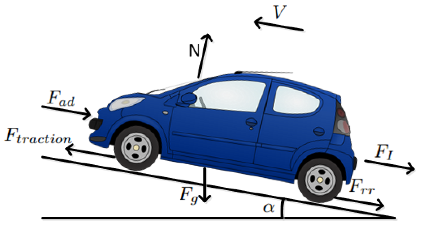
We consider a force model consisting of the gravitational force, aerodynamic drag, rolling resistance, and inertial force, as shown in Figure 1. In particular, the gravitational force is given by
where is the road slope, g is the gravity of earth, and m is the vehicle mass. The aerodynamic drag force is given by
where is the air density, A is the vehicle frontal area, is the vehicle form coefficient, and v is the velocity. The rolling resistance force is given by
where is the static resistance coefficient and is the dynamic resistance coefficient. The inertial force is given by
where a is the acceleration, I is the shaft moment of inertia, G is the gear ratio, and is the wheels radius. In general, G is a function of the driving speed. In the case of an EV, the gear ratio should be replaced with a constant. The sum of the forces equals the traction effort extracted by the motor, , and satisfies
2.2. Powertrain Model
The powertrain supplies the power from the battery to the wheels, which provides the required traction force according to Equation (6). The powertrain considers the gear box, the shaft, the three-phase AC motor, the inverter, and the regenerative braking mechanism. Nonlinear motor efficiency, , and gear-box discontinuity should be taken into account in order to calculate the power extracted from the battery. A standard motor efficiency map and a four gears transmission system were implemented based on [32]. According to those models, both gear ratio selection and motor efficiency are functions of velocity. The motor torque, , and the motor angular velocity, , are given by
and
respectively, where is the gear efficiency. The power consumed from the battery, , is therefore known and can be expressed by
where is the inverter efficiency. The inverter and gear efficiencies are assumed to be constant. By substituting Equations (7) and (8) into Equation (9), one obtains
In cases of negative , generally when decelerating, energy can be used for recharging the battery. This regenerative braking mechanism [33] changes to in the powertrain model from Equation (10). The generator effectiveness, , is relatively low due to the additional mechanical braking and is assumed to be constant [33].
2.3. Travel Time and Energy Consumption Models
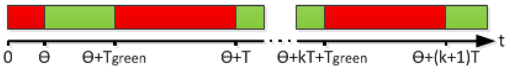
In this subsection, the travel time and energy consumption models are defined in terms of vehicle velocity and the traffic light model. These models describe a multi-segment and single vehicle problem. In urban environments, energy consumption is subject to traffic light status. When arriving at a red light, the driver is forced to stop, and this significantly increases energy consumption and travel time. In this paper, these stops are considered as time and energy penalties. The traffic signal status at each intersection is assumed to be periodic, with a specified time offset, green time, and cycle duration at each intersection. The typical traffic signal status is presented in Figure 2, where T is the period time, the green light timing is within the first seconds, the phase offset from time zero is , and k is the number of complete cycles that have passed from an arbitrary initial time until the vehicle arrives at intersection i, which can be referred to as the green window number.
According to this traffic light model, the ith intersection is at the end of segment i and the intersection arriving time, , when the traffic light is green, satisfying
The number of the green cycle that the car uses at intersection i, , is given by
where is an integer division.
For the sake of simplicity, a standard driving profile [2,34] is used in this paper. According to the driving profile, the route is divided into several segments, where each segment ends with a traffic light and has a target speed. Then, each segment is divided into two intervals: transition and steady-state intervals. During the transition interval, the vehicle accelerates to the target speed of the segment. Since optimal speed planning will often result in not stopping at red lights, the acceleration is assumed to be relativity small and the duration of the acceleration phase is the same for each segment and defined by . This assumption simplifies the driving model but neglects constraints for the maximum power, as well as jerk constraint for driving comfort. The value of parameter can vary for different vehicles and is dependent on the vehicle’s acceleration performance and the maximum speed limit. Then, as part of the steady-state interval, the vehicle travels at a constant speed for the remainder of the segment. Thus, the acceleration at time t is given by
The distance covered in the transition interval is
The travel time of each segment, consisting of the transition and steady-state times, is given by
In the case where the vehicle has not stopped at a red light, the arrival time at the ith intersection is obtained by summing the travel time of each segment, as presented in Equation (16):
where is the velocity vector for the N-segment route and is the initial time.
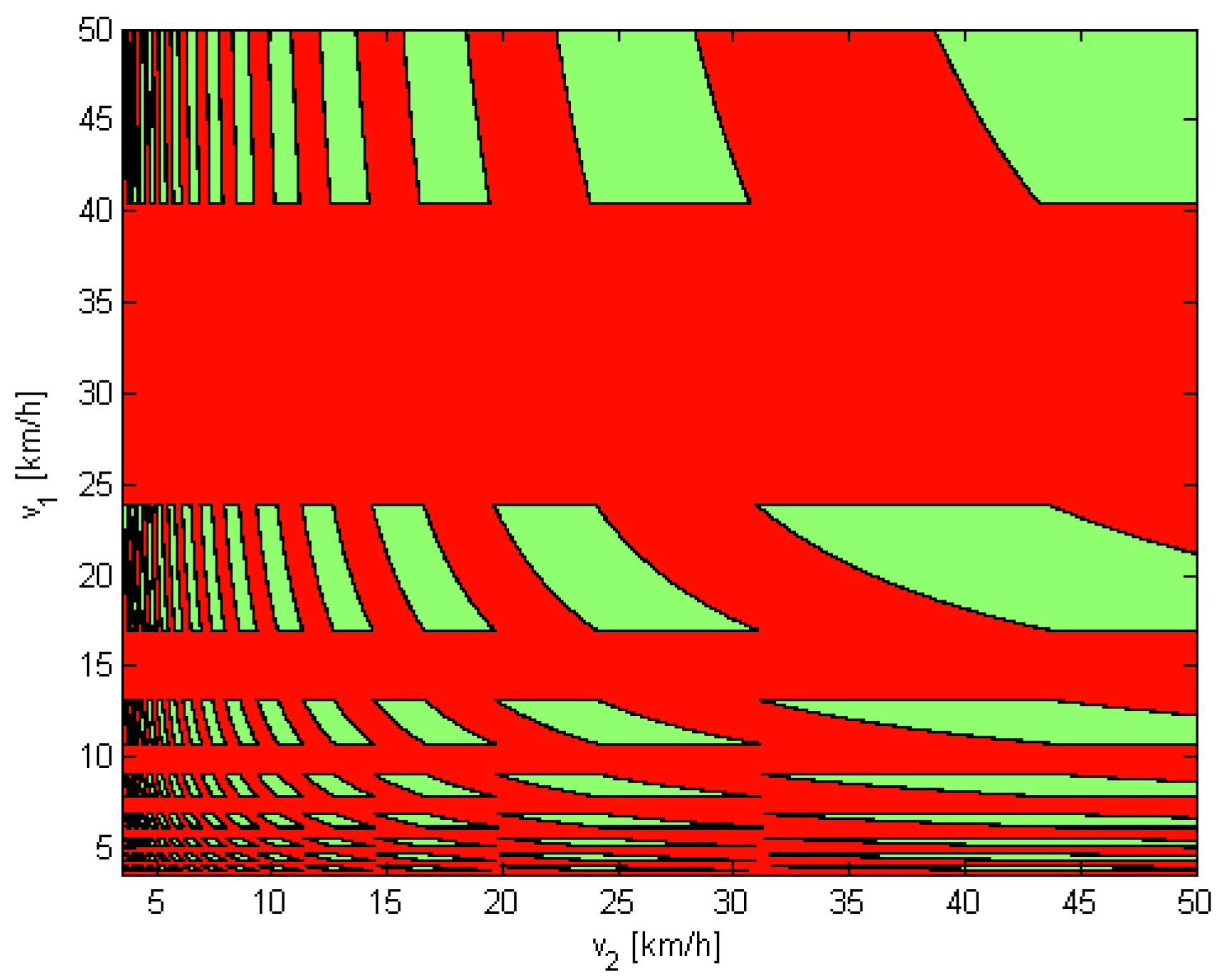
An example of a traffic light status map for a two-segment route is presented in Figure 3 with the parameters in Table 3, for and . The green windows (when the vehicle arrives at both intersections at a green light) demonstrate the problem’s complexity. Figure 3 shows that the traffic light condition from Equation (11) is neither a convex nor a continuous set. It can be seen that the vehicle will encounter green lights at the intersection at the end of the first segment if it drives, for example, at km/h or km/h. If it drives with km/h, to encounter green lights at the second intersection, it could drive at, for example, at 45 or 25 km/h.
The travel time in Equation (16) is calculated without taking the vehicle stops into account. The time stops penalties are caused by the idling time until the traffic light turns green, and satisfies
where the deceleration time before the red light is considered as part of the waiting time and the stopping condition for each intersection, , is based on Equation (11) and is given by
The total travel time, , is obtained by summing up the travel time from Equation (16) and the time stopping penalty from Equation (18) in each segment from the segments set, , in an N-segment route:
The energy consumption calculations consider both the auxiliary loads energy and the energy that is used for driving. Auxiliary loads power, , which includes radio, air conditioning, lights, and electrical control units, is assumed to be constant [30]. Therefore, the auxiliary loads energy is related to the total travel time and is given by
The driving energy consumption is calculated by a numerical integration of power over time. According to the presented profile, each segment is divided into intervals, in which the battery power from Equation (10) is assumed to be constant. Therefore, the energy consumed in the transition interval is
where is the segment slope that is assumed to be constant for each segment. Although the velocity during the transition interval is not constant, an average value of is considered in the power calculation from Equation (10). This approximation is relatively minor since and are close to GLOSA systems, as the vehicle does not stop at red lights. The full equation is presented in Equation (28). In the remaining distance, , the vehicle maintains a constant speed until the next traffic light. Thus, the energy consumed in this steady-state interval is given by
In cases when the vehicle stops, the total energy includes a stop penalty term that consists of two contributions: the vehicle stop and the re-acceleration that replaces the transition interval in Equation (23). Therefore, the energy consumption penalty satisfies
The total energy consumption, , is obtained by summing the intervals energies in Equations (23)–(25), which results in
3. Optimization Problem Formulation
Traffic light timing data enable an optimal speed planning that minimizes energy consumption and travel time. With this goal in mind, an appropriate objective function should be defined and optimization tools should be used to find the associated global optimum. In this paper, we consider a multiobjective function [17] that consists of total travel time from Equation (21) and energy consumption from Equation (28). In particular, the objective function is defined as:
where is a tuning parameter that controls the trade-off between energy consumption and travel time costs, and is set as the time coefficient in order to quantify the time relative to the energy. Assuming that the vehicle turns the engine off while standstill (which is very common in EVs), C will be equal to Paux. The objective function is in terms of energy, but considers an adjustable trade-off between the energy and time. By substituting Equation (27) into Equation (29) and setting for simplification, the following GLOSA system objective function is obtained:
It can be seen in Equation (30) that the objective function increases when the energy or the travel time increases. The advisory speed vector, V, must be between the minimum and maximum speed limits, and , respectively. Therefore, the GLOSA system’s optimization problem can be formulated as:
Traffic light discontinuity, which is presented in Equation (11), results in a discontinuous stop penalty. Thus, the objective function turns out to be a nonconvex discontinuous function. The function complexity makes it impractical to solve with standard optimization toolboxes and in a reasonable computation time [17].
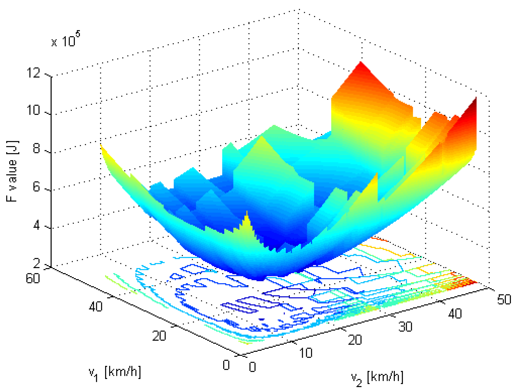
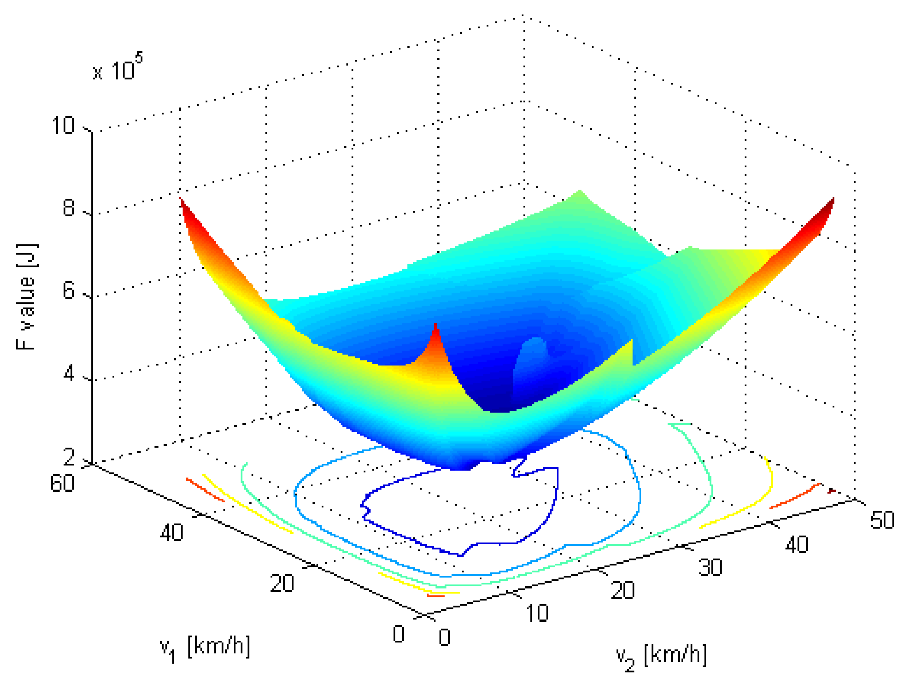
An example of the proposed objective function for a two-segment route is presented in Figure 4 for , , and the parameters of the traffic light status map as presented in Figure 3. The green windows from this map are reflected directly in the objective function shadows, demonstrating the direct relation between them. The stopping penalties can be viewed as the major jumps in the objective function. The objective function shows that slow driving is reflected as an increase in F values as travel time increases. Fast driving is also not optimal due to high energy consumption.
4. Dynamic-GLOSA
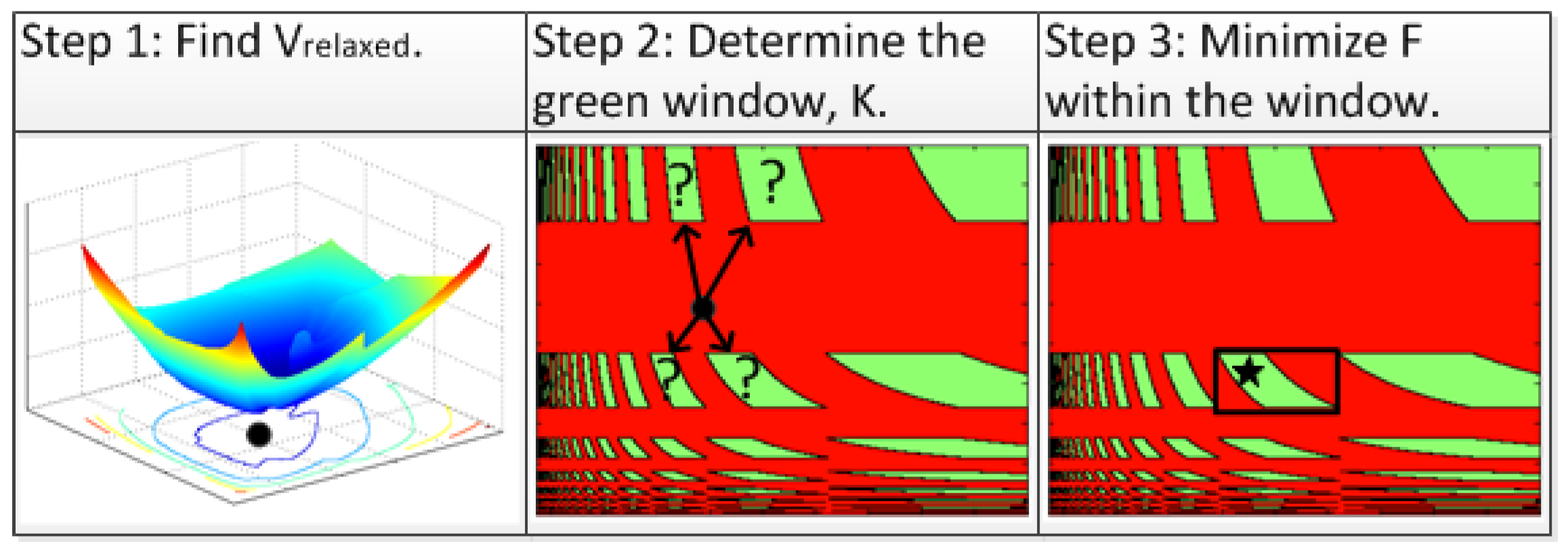
The optimization problem from Equation (31) is a nonconvex optimization problem that is intractable in real time scenarios. This section presents a real-time algorithm based on a relaxation procedure for solving the GLOSA optimization problem and offers improved optimization results and reduced calculation time. The algorithm, referred to as Dynamic-GLOSA, and the proposed method assume that avoiding stops is preferable to stopping at red lights. This assumption has been proven using a brute force search that seeks the true optimal driving profile. However, an edge case in which this assumption is invalid may occur. Based on that, a solution in three main steps is suggested.
According to the first step of the proposed algorithm, the traffic light status can be expressed indirectly and the objective function from Equation (30) is calculated without taking the traffic light stop penalties into consideration. Therefore, the relaxed objective function is given by substituting Equations (21) and (26) into Equation (30) and substituting for each intersection:
It can be seen that the relaxed objective function from Equation (32), as presented in Figure 5, does not contain the major discontinuities caused by the traffic lights as in the original objective function from Equation (30), as presented in Figure 4. This modified model is still non-convex due to factors such as gear switching and motor efficiency. However, as the Results Section demonstrates, this relaxation can be assumed not to affect the approximation of the global optimum that was calculated using a brute force search. Furthermore, the relaxation procedure enables the solution for this step to be found in real-time by using standard optimization toolboxes, which should make the implementation of this method easier [35]. This partial solution describes the optimal driving speeds of the relaxed problem, , and is not really the optimal solution because it does not comply with the traffic light constraints in the real world (which are taken into account in the next steps).
The second step of the proposed method considers the traffic light status and selects the green window for passing through each intersection. The green window is described by , and should be determined according to Equation (12). The objective function from Equation (30) indicates that the green window, K, should be as close as possible to the relaxed optimal speed in each segment. In the case where the vehicle will arrive at the intersection when there is a green light, the velocity will be the advisory speed. In the case of arriving when there is a red light, two values are tested: before and after the relaxed optimal speed for the segment. These window values are given by
and
In general, more values will improve the results but will increase the calculation time significantly. In this paper, the choice of two values for is proved to show satisfactory optimization results. Each of these windows reflects a different driving speed in order to arrive in the middle of the green phase:
and
According to the second step, the green widow selection is done from the first segment to the last. First, the objective function value is calculated for two of the close green windows by setting and . Second, the segment green window with the lowest objective function value is selected for the specific segment. Then, this step is repeated for each segment until K is determined. The search complexity is linear (), and as such it enables a short calculation time for multi-segment cases.
In the third and last step, after the green windows have been determined, each segment passing time is within a specific cycle: . Calculating the optimal speeds within this window can be done by using standard optimization tools, due to the significant reduction in problem complexity. Finally, the proposed GLOSA-dynamic algorithm is summarized in Algorithm 1 and visualized in Figure 6.
| Algorithm 1 Dynamic-GLOSA algorithm. |
|
5. Simulation Results
In this section, the performance of the proposed Dynamic-GLOSA algorithm is evaluated for different methods and driving patterns.
5.1. Methods and Parameters
The Dynamic-GLOSA solution was compared with the optimal solution and with the performance of the following methods:
- BF-GLOSA: A brute force (BF) search is implemented to calculate the optimal solution of the optimization problem in Equation (31). The BF is time consuming and has computational complexity that grows exponentially with the number of segments. Thus, this search is impractical and is possible only in scenarios with a low number of road segments.
- GA-GLOSA [13]: This Genetic Algorithm (GA) statistically generates solutions, compares their scores, and selects the best solution [36]. This process is repeated several times to increase the natural selection. The parameters of the GA, including the genetic natural selection, score function, and mutations, are implemented according to the values in [13].
- Naive driver: The naive driver is an unassisted driver who travels at a constant velocity. In the following, the naive driver velocity is set at 34 km/h according to the average driving speed in the New European Driving Cycle (NEDC) profile [37] and the driver stops at the intersection when the light is red. The naive driver uses a naive strategy that is likely to be worse than that of real and intelligent drivers. The naive driver is used as a benchmark in order to evaluate the energy and time saving potential by using GLOSA.
The vehicle model parameters presented in Table 1 were based on [30,31]. These parameters reflect a small EV model adjusted for urban conditions. The route parameters were based on the NEDC model [37], which is characterized by short segments and includes 13 stops. To generate generic simulations, the route parameters were drawn according to a uniform random distribution, , where the specific ranges for each parameter were set according to Table 2. The transition time, the initial time, and the initial speed were set to be s, , and , respectively. The constant auxiliary power consumption was assumed to be .
In this research, was used to minimize the objective function. The simulations were performed on a standard laptop, with Intel(R) Core(TM) 2 Duo CPU, T9550 2.66 Ghz.
5.2. Typical Solution
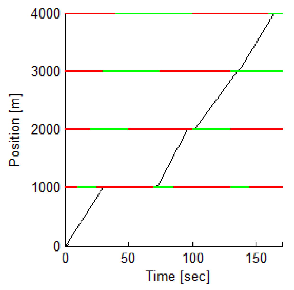
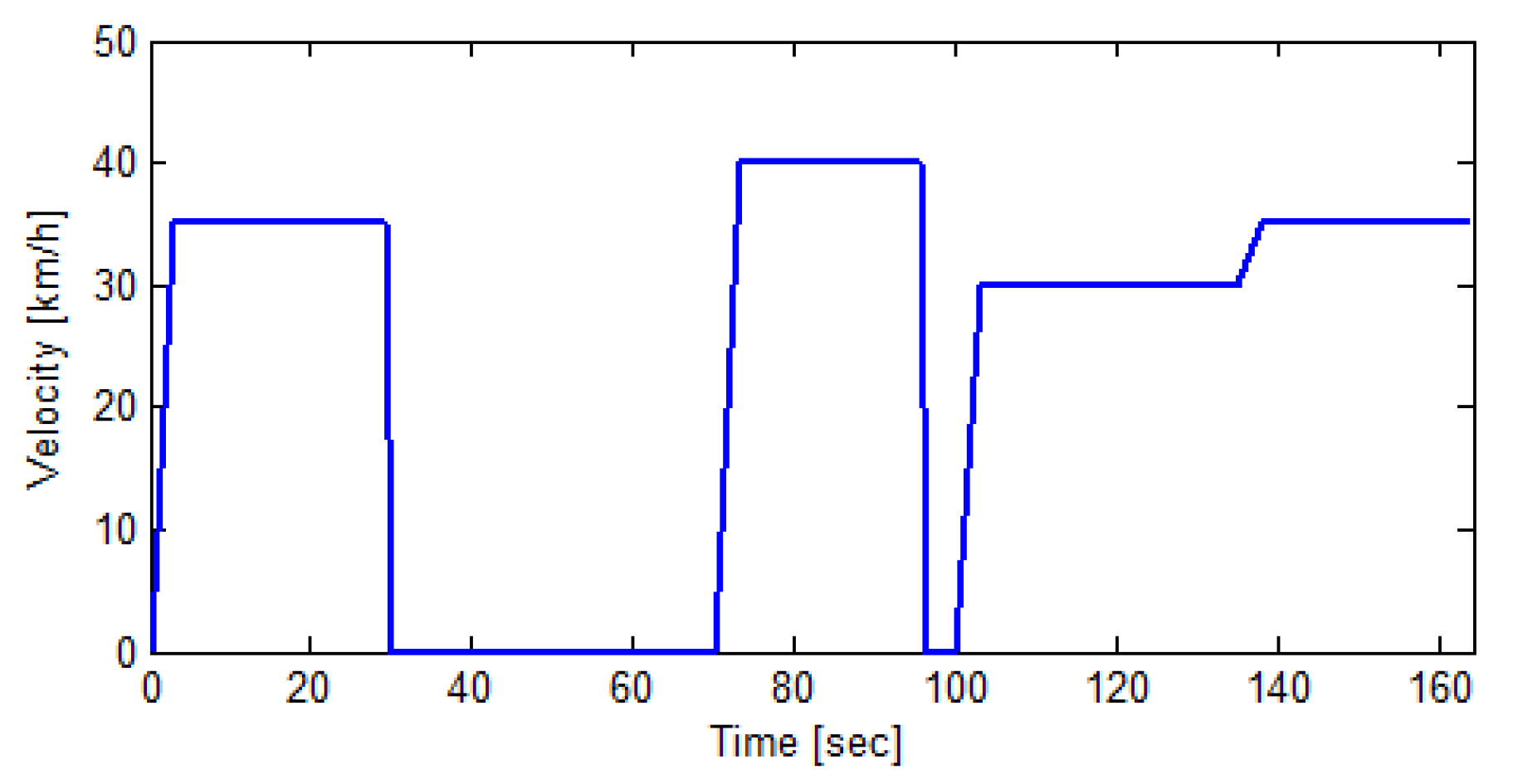
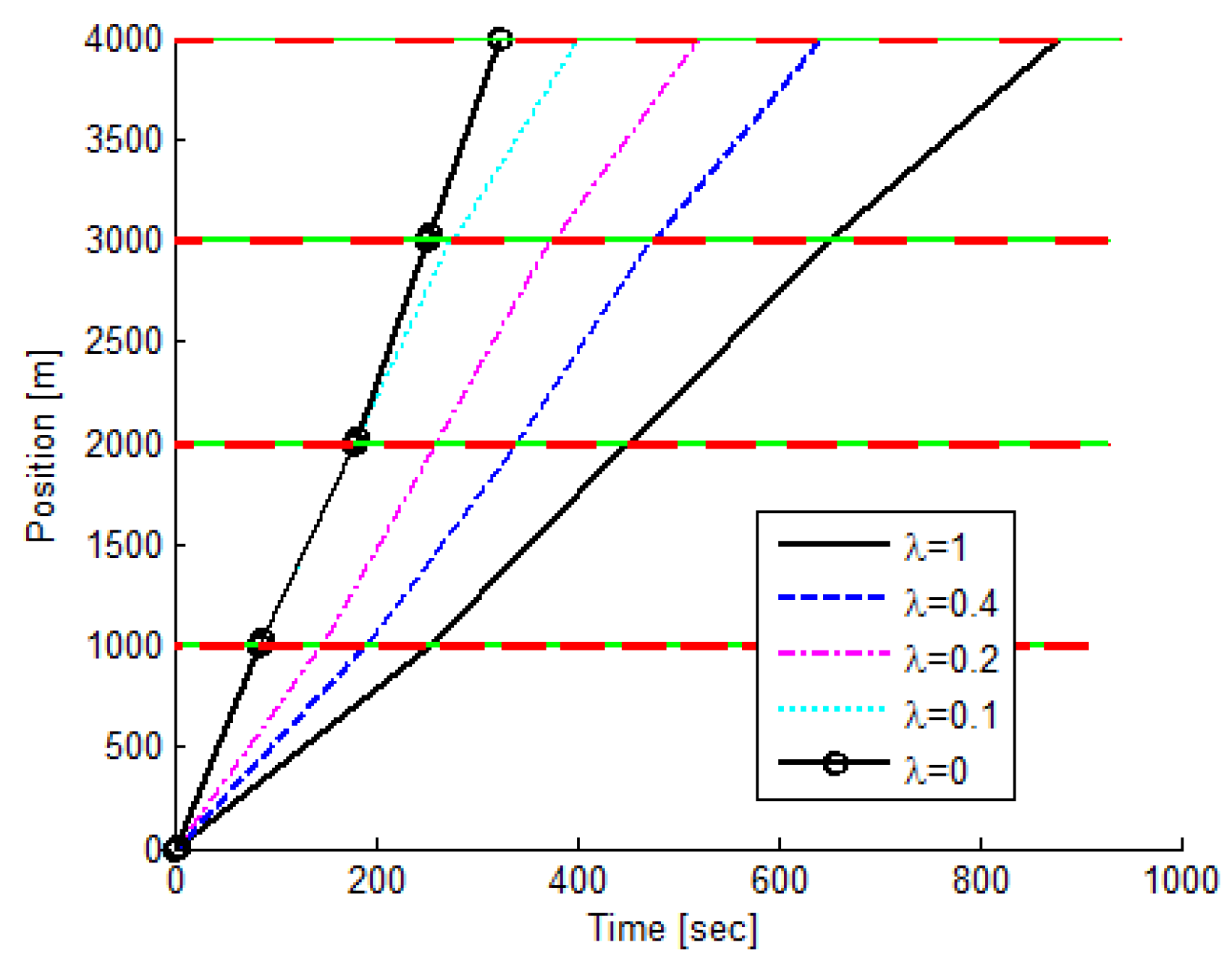
This subsection presents a typical speed profile for a four-segment route, based on the driving profile from the previous subsections. The smoothness of the generated speed trajectory can be seen in the given example. Each segment was divided into three intervals: transition, steady-state, and stopping intervals. The travel times which each interval takes are given by , Equations (16), and (18), respectively. The energy consumption in each of these intervals is calculated by Equations (23)–(25), respectively. The vehicle parameters used for this simulation are in accordance with Table 1, and the arbitrary route parameters are presented in Table 3 and can be seen in Figure 7. It should be noted that the intersection can be defined by different parameters sets, which can imply different sizes of intersections or approaches from a side road to a main road. Therefore, the parameters for each intersection were drawn randomly to ensure generic simulations for comparison. The initial time and the initial speed can be set to any values, but, to simplify the calculation, they were set to and , respectively. The velocities vector was set to , and the transition time was set at . The driving profile example is given in detail in Table 4, where the division of the intervals is presented.
According to the given velocities vector for the given example, the vehicle will stop at the first and second intersections. Figure 7 and Figure 8 show that these stops are described by traffic light stop and idling intervals. For the presented route and velocities vector, the total energy consumption is Joules and the total travel time is s.
5.3. Energy and Time Trade-Off
The objective function from Equation (30) is a function of the parameter that represents the trade-off between energy consumption and travel time. The forces equation from Equation (6) presents an increasing function depending on the velocity v, which reflects the increasing nature of the energy consumption in Equation (26). It can be seen that the total travel time from Equation (16) is a decreasing function depending on the velocity v, due to the inverse relation. Therefore, one contradicts the other and an energy/time trade-off must be determined according to a specific criterion. The trade-off value is increased to attribute more weight to the energy saving, while its decrease indicates a higher weight attributed to the time criterion.
The energy consumption and travel time results for a four-segment route, calculated by the BF-GLOSA solution, are presented in Table 5 for . The optimal driving strategies were calculated for the same route and relate to the different values of in Figure 9.
Figure 9 and Table 5 demonstrate that, for a small value of , the travel time decreases. In particular, for , the shortest travel time and highest energy consumption are obtained. Conversely, as increases, the energy consumption decreases. Therefore, the value of should be chosen according to the desired trade-off between time and energy. The quantitative relationship of this trade-off is discussed in [38].
Different values for were tested to demonstrate each method’s behavior. In the following simulation, different values of from 0 to 1 were tested, and the energy and time results of each method were calculated based on the advisory speed profile and according to Equations (21) and (26). Then, a Pareto front was derived from the results to show the quantitative relationship between energy consumption and travel time. As in the previous simulation, this simulation was based on fixed and arbitrary route parameters that are presented in Table 3.
In Figure 10, it can be seen that, for every value of , the BF-GLOSA, which represents the optimal solution, and Dynamic-GLOSA are better than the other methods. It can also be seen that the Dynamic-GLOSA results approach those of the BF-GLOSA. The GA-GLOSA and MAX-GLOSA methods perform well in terms of travel time optimization, but their performance decreases as increases. The GA-GLOSA method uses a random algorithm, thus it is not smooth [36]. The MAX-GLOSA and naive driver results are reflected as dots since is not considered as part of the velocity calculation.
5.4. Optimization Results
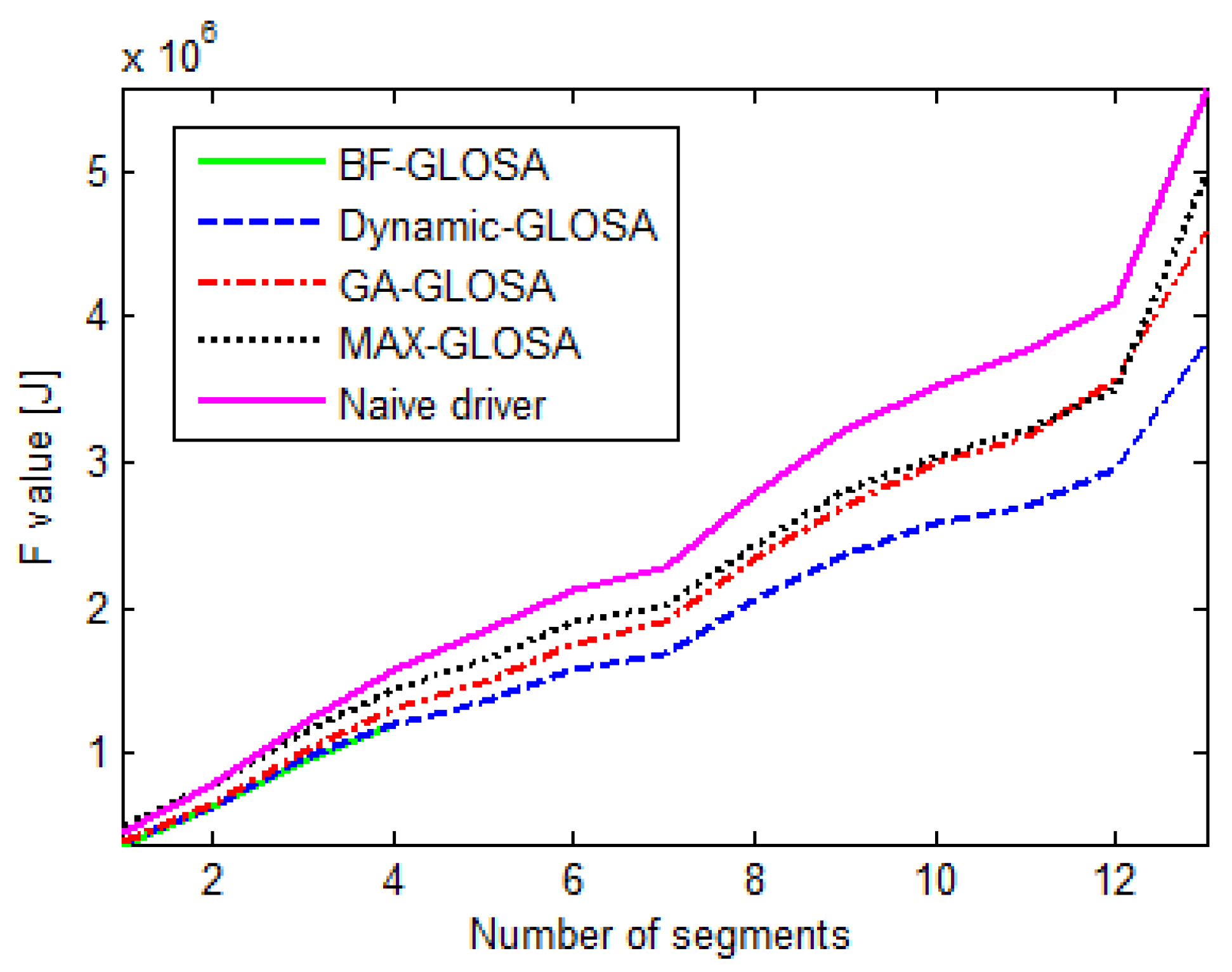
Next, 100 Monte-Carlo [39] simulations were run for different numbers of segments. First, the route parameters were drawn randomly according to Table 2 and the parameters in Section 5.1. Second, the advisory speed profile of each method was evaluated based on the methods presented in Section 5.1. Finally, the objective function value for each method was calculated based on the advisory speed profile and the objective function from Equation (30) and the average results were calculated. In the following simulations, parameter was set to 0.2 to stress the importance of the energy criterion.
As expected, Figure 11 illustrates that F value increases as the number of segments increases. This simulation compares the described methods and shows that the Dynamic-GLOSA results are better than the other benchmark methods for every number of segments. A similar comparison in [40] shows that a Genetic Algorithm such as the GA-GLOSA is preferable to other methods. In addition, it can be seen that the performance of the proposed Dynamic-GLOSA algorithm is very close to the BF-GLOSA optimal solution. The optimal solution was not calculated for more than four segments because of the high complexity and the unrealistic calculation time.
In Table 6, the simulation results for the four-segment case are compared with the optimal BF-GLOSA solution. In this simulation, the advisory speed profile was calculated according to each method for 100 random scenarios. Following this, the same profiles were used to calculate the methods’ objective function values from Equation (30), F, the travel time from Equation (21), T, the energy consumption from Equation (26), E, and the computational complexity, i.e., calculation time.
Table 6 illustrates that, as expected, the BF-GLOSA solution has the lowest cost, F. The Dynamic-GLOSA F values are relatively close to the optimal BF-GLOSA solution, with only a 1.01% higher cost and a small variance of 1.96%. The Dynamic-GLOSA average calculation time, , allows real-time implementation. The GA-GLOSA shows reasonable optimization results but requires a lengthy calculation time. An overly simplified model, such as MAX-GLOSA, displays a short calculation time, but the objective function results are unsatisfying as the vehicle model is not taken into account. The naive driver solution presents both the highest energy consumption and the longest travel time. By comparison with the naive driver, the Dynamic-GLOSA consumes 50.2% less energy and takes 6.4% less travel time. The Dynamic-GLOSA results show that the energy saving is more significant than the travel time saving, because the objective function trade-off in this paper considers energy to be more important.
The 13-segment case was also tested, as the problem complexity grows significantly with the number of segments. The average objective function values, travel time, energy consumption, and calculation time are presented in Table 7 for 100 Monte-Carlo simulations and a 13-segment route. This simulation compared the Dynamic-GLOSA, GA-GLOSA, MAX-GLOSA, and the naive driver methods. The optimal BF-GLOSA solution was not calculated due to unrealistic calculation time.
Similar to the results for the four-segment case, the objective function values for the Dynamic-GLOSA method are lower than for the other methods. Compared to the naive driver method, the Dynamic-GLOSA method presents 38.1% energy saving potential. The Dynamic-GLOSA calculation time remains relatively low even for the 13-segment route. Since changes in traffic are relatively slow, the calculation time results, together with the use of standard laptop and standard optimization toolbox, show that the method can run in real time with a vehicle equipped with a standard on-board computer.
6. Conclusions
In this paper, we investigate the optimization problem of the GLOSA system and propose a real-time solution. A new formulation of the GLOSA system is introduced that includes energy consumption, travel time, and traffic light models. In urban environments, stopping at traffic lights usually occurs without the use of preliminary information and, therefore, the energy consumption of an unassisted driver increases. In general, the energy saving potential increases when driving is based on a more sophisticated algorithm. The optimization problem is reformulated and it is now emphasized that the GLOSA optimization problem is a nonconvex optimization problem, due to the traffic light discontinuity, which is intractable in real time scenarios. Based on a smoother relaxation procedure for this problem, a dynamic real-time algorithm is presented with a high degree of optimization and low calculation time that can be used with all types of vehicles. Simulations showed that the performance of the proposed Dynamic-GLOSA algorithm is very close to that with optimal driving speeds obtained by the brute-force solution but with a much shorter calculation time. In addition, the proposed Dynamic-GLOSA driving strategy advisory was demonstrated to be better than existing methods for every number of segments and every time and energy trade-off value investigated, but is much superior in terms of energy saving potential. Due to the short calculation time in the Dynamic GLOSA method, a real-time implementation for the Dynamic-GLOSA is possible.
The paper deals with the mathematical challenges in calculating the optimal speed and presents a new mathematical approach, which proves capable of reducing calculation time and approximating the optimal solution. Future researchers can employ the presented method as the mathematical substrate for a real-time implementation to meet real-world randomness [41] and to avoid cumulated errors [26,27]. The proposed method can be extended for multiple vehicle solutions, for example by using vehicle-to-vehicle communication (V2V) [23]. By using V2X communication, information about nearby traffic can be analyzed in real time and used to recalculate the optimal driving profile.
Author Contributions
Research and writing, L.S.; and Supervision, R.R. All authors have read and agreed to the published version of the manuscript.
Funding
The author wishes to thank the Israeli Ministry of National Infrastructures, Energy, and Water Resources for its financial support.
Acknowledgments
The author would like to express his deep gratitude to Tirza Routtenberg for her inspirational guidance, unflagging encouragement, and professional assistance, which brought this research to fruition.
Conflicts of Interest
The authors declare no conflict of interest. The funders had no role in the design of the study; in the collection, analyses, or interpretation of data; in the writing of the manuscript, or in the decision to publish the results.
References
- International Energy Agency. Capturing the Multiple Benefits of Energy Efficiency; International Energy Agency: Paris, France, 2014. [Google Scholar]
- Zhang, R.; Yao, E. Eco-driving at signalised intersections for electric vehicles. IET Intell. Transp. Syst. 2015, 9, 488–497. [Google Scholar] [CrossRef]
- Younes, Z.; Boudet, L.; Suard, F.; Gerard, M.; Rioux, R. Analysis of the main factors influencing the energy consumption of electric vehicles. In Proceedings of the International Electric Machines & Drives Conference (IEMDC), Chicago, IL, USA, 12–15 May 2013; pp. 247–253. [Google Scholar]
- Salman, A.; Cohen, Y.; Simchon, L.; Routtenberg, T.; Rabinovici, R. Optimal switching in a three-level inverter: An analytical approach. In Proceedings of the International Conference on the Science of Electrical Engineering (ICSEE), Eilat, Israel, 16–18 November 2016; pp. 1–5. [Google Scholar]
- De Nunzio, G.; Wit, C.C.; Moulin, P.; Di Domenico, D. Eco-driving in urban traffic networks using traffic signals information. Int. J. Robust Nonlinear Control. 2016, 26, 1307–1324. [Google Scholar] [CrossRef] [Green Version]
- Guardiola, C.; Pla, B.; Pandey, V.; Burke, R. On the potential of traffic light information availability for reducing fuel consumption and NOx emissions of a diesel light-duty vehicle. Proc. Inst. Mech. Eng. Part D J. Automob. Eng. 2019. [Google Scholar] [CrossRef]
- Asadi, B.; Vahidi, A. Predictive cruise control: Utilizing upcoming traffic signal information for improving fuel economy and reducing trip time. Trans. Control Syst. Technol. 2011, 19, 707–714. [Google Scholar] [CrossRef]
- Yin, B.; Dridi, M.; El Moudni, A. Adaptive Traffic Signal Control for Multi-intersection Based on Microscopic Model. In Proceedings of the 27th International Conference on Tools with Artificial Intelligence (ICTAI), Mare, Italy, 9–11 November 2015; pp. 49–55. [Google Scholar]
- Zaidi, A.A.; Kulcsar, B.; Wymeersch, H. Traffic-adaptive signal control and vehicle routing using a decentralized back-pressure method. In Proceedings of the European Control Conference (ECC), Linz, Austria, 15–17 July 2015; pp. 3029–3034. [Google Scholar]
- Protschky, V.; Feld, S.; Walischmiller, M. Traffic Signal Adaptive Routing. In Proceedings of the 18th International Conference on Intelligent Transportation Systems (ITSC), Canaria, Spain, 15–18 September 2015; pp. 450–456. [Google Scholar]
- Yang, Z.; Lu, S.; Liu, X. Combined traffic signal control and route guidance: multiple user class traffic assignment model versus discrete choice model. In Proceedings of the IMACS Multiconference on Computational Engineering in Systems Applications, Beijing, China, 4–6 October 2006; pp. 1957–1964. [Google Scholar]
- Katsaros, K.; Kernchen, R.; Dianati, M.; Rieck, D. Performance study of a Green Light Optimized Speed Advisory (GLOSA) application using an integrated cooperative ITS simulation platform. In Proceedings of the 7th International Wireless Communications and Mobile Computing Conference (IWCMC), Istanbul, Turkey, 4–8 July 2011; pp. 918–923. [Google Scholar]
- Seredynski, M.; Mazurczyk, W.; Khadraoui, D. Multi-segment green light optimal speed advisory. In Proceedings of the 27th International Parallel and Distributed Processing Symposium Workshops & PhD Forum (IPDPSW), Boston, MA, USA, 20–24 May 2013; pp. 459–465. [Google Scholar]
- Guan, T.; Frey, C.W. Predictive fuel efficiency optimization using traffic light timings and fuel consumption model. In Proceedings of the 16th International IEEE Conference on Intelligent Transportation Systems-(ITSC), The Hague, The Netherlands, 6–9 October 2013; pp. 1553–1558. [Google Scholar]
- Suramardhana, T.A.; Jeong, H.Y. A driver-centric green light optimal speed advisory (DC-GLOSA) for improving road traffic congestion at urban intersections. In Proceedings of the Asia Pacific Conference on Wireless and Mobile, Bali, Indonesia, 28–30 August 2014; pp. 304–309. [Google Scholar]
- Protschky, V.; Feit, S.; Linnhoff-Popien, C. Extensive traffic light prediction under real-world conditions. In Proceedings of the 80th Vehicular Technology Conference (VTC Fall), Vancouver, BC, USA, 14–17 September 2014; pp. 1–5. [Google Scholar]
- Boyd, S.; Vandenberghe, L. Convex Optimization; Cambridge University Press: Cambridge, UK, 2004. [Google Scholar]
- Xiang, X.; Zhou, K.; Zhang, W.B.; Qin, W.; Mao, Q. A Closed-Loop Speed Advisory Model with Driver’s Behavior Adaptability for Eco-Driving. IEEE Trans. Intell. Transp. Syst. 2015, 16, 3313–3324. [Google Scholar] [CrossRef]
- Wu, X.; He, X.; Yu, G.; Harmandayan, A.; Wang, Y. Energy-optimal speed control for electric vehicles on signalized arterials. IEEE Trans. Intell. Transp. Syst. 2015, 16, 2786–2796. [Google Scholar] [CrossRef]
- Dahmen, T.; Saupe, D. Calibration of a power-speed-model for road cycling using real power and height data. Int. J. Comput. Sci. Sport 2011, 10, 18–36. [Google Scholar]
- Gong, S.; Shen, J.; Du, L. Constrained optimization and distributed computation based car following control of a connected and autonomous vehicle platoon. Transp. Res. Part B Methodol. 2016, 94, 314–334. [Google Scholar] [CrossRef]
- Stebbins, S.; Hickman, M.; Kim, J.; Vu, H.L. Characterising green light optimal speed advisory trajectories for platoon-based optimisation. Transp. Res. Part C Emerg. Technol. 2017, 82, 43–62. [Google Scholar] [CrossRef]
- HomChaudhuri, B.; Pisu, P. A Control Strategy for Driver Specific Driver Assistant System to Improve Fuel Economy of Connected Vehicles in Urban Roads. In Proceedings of the 2019 American Control Conference (ACC), Philadelphia, PA, USA, 10–12 July 2019; pp. 5557–5562. [Google Scholar]
- Wei, Z.; Hao, P.; Barth, M.J. Developing an Adaptive Strategy for Connected Eco-Driving under Uncertain Traffic Condition. In Proceedings of the 2019 IEEE Intelligent Vehicles Symposium (IV), Paris, France, 9–12 June 2019; pp. 2066–2071. [Google Scholar]
- Jiang, H.; Hu, J.; Park, B.B.; Wang, M.; Zhou, W. An extensive investigation of an eco-approach controller under a partially connected and automated vehicle environment. Sustainability 2019, 11, 6319. [Google Scholar] [CrossRef] [Green Version]
- Hao, P.; Wu, G.; Boriboonsomsin, K.; Barth, M.J. Eco-approach and departure (EAD) application for actuated signals in real-world traffic. IEEE Trans. Intell. Transp. Syst. 2018, 20, 30–40. [Google Scholar] [CrossRef]
- Almannaa, M.H.; Chen, H.; Rakha, H.A.; Loulizi, A.; El-Shawarby, I. Field implementation and testing of an automated eco-cooperative adaptive cruise control system in the vicinity of signalized intersections. Transp. Res. Part D Transp. Environ. 2019, 67, 244–262. [Google Scholar] [CrossRef]
- Zhao, N.; Roberts, C.; Hillmansen, S.; Nicholson, G. A multiple train trajectory optimization to minimize energy consumption and delay. IEEE Trans. Intell. Transp. Syst. 2015, 16, 2363–2372. [Google Scholar] [CrossRef]
- Wang, F.; Tang, K.; Li, K. Stochastic effects of traffic randomness on the determination of signal change and clearance intervals at signalised intersections. IET Intell. Transp. Syst. 2014, 9, 250–263. [Google Scholar] [CrossRef]
- Schaltz, E. Electrical Vehicle Design and Modeling; INTECH Open Access Publisher: London, UK, 2011. [Google Scholar]
- Kaloko, B.S.; Soebagio, M.H.P.; Purnomo, M.H. Design and Development of Small Electric Vehicle using MATLAB/Simulink. Int. J. Comput. Appl. 2011, 24, 19–23. [Google Scholar] [CrossRef]
- Ren, Q.; Crolla, D.; Morris, A. Effect of transmission design on electric vehicle (EV) performance. In Proceedings of the IEEE Vehicle Power and Propulsion Conference, Dearborn, MN, USA, 7–11 September 2009; pp. 1260–1265. [Google Scholar]
- Ceuca, E.; Tulbure, A.; Risteiu, M. The evaluation of regenerative braking energy. In Proceedings of the 16th International Symposium for Design and Technology in Electronic Packaging (SIITME), Pitesti, Romania, 23–26 September 2010; pp. 65–68. [Google Scholar]
- Corti, A.; Manzoni, V.; Savaresi, S.M. Simulation of the impact of traffic lights placement on vehicle’s energy consumption and CO2 emissions. In Proceedings of the 15th International Conference on Intelligent Transportation Systems (ITSC), Anchorage, AK, USA, 16–19 September 2012; pp. 620–625. [Google Scholar]
- Osborne, M.J. Quasiconcavity and quasiconvexity. In Mathematical Methods for Economic Theory: A Tutorial; University of Toronto: Toronto, ON, Cananda, 2007; Chapter 3.4. [Google Scholar]
- Mitchell, M. An Introduction to Genetic Algorithms; MIT Press: Cambridge, MA, USA, 1998. [Google Scholar]
- Silva, C.; Ross, M.; Farias, T. Evaluation of energy consumption, emissions and cost of plug-in hybrid vehicles. Energy Convers. Manag. 2009, 50, 1635–1643. [Google Scholar] [CrossRef]
- Li, L.; Dong, W.; Ji, Y.; Zhang, Z.; Tong, L. Minimal-energy driving strategy for high-speed electric train with hybrid system model. IEEE Trans. Intell. Transp. Syst. 2013, 14, 1642–1653. [Google Scholar] [CrossRef]
- Raychaudhuri, S. Introduction to monte carlo simulation. In Proceedings of the 2008 Winter Simulation Conference, Miami, FL, USA, 7–10 Decembe 2008; pp. 91–100. [Google Scholar]
- Seredynski, M.; Dorronsoro, B.; Khadraoui, D. Comparison of green light optimal speed advisory approaches. In Proceedings of the 16th International Conference on Intelligent Transportation Systems (ITSC), The Hague, The Netherlands, 6–9 October 2013; pp. 2187–2192. [Google Scholar]
- Meng, X.; Cassandras, C.G. A Real-Time Optimal Eco-driving for Autonomous Vehicles Crossing Multiple Signalized Intersections. arXiv 2019, arXiv:1901.11423. [Google Scholar]
Figure 1.
Forces applied on a vehicle.

Figure 2.
Traffic light model: status versus time.

Figure 3.
Traffic light status map for a two-segment route.

Figure 4.
The nonconvex objective function versus the velocity for a two-segment route and the GLOSA system optimization problem.
Figure 4.
The nonconvex objective function versus the velocity for a two-segment route and the GLOSA system optimization problem.

Figure 5.
The relaxed objective function versus the velocity for a two-segment route.

Figure 6.
The Dynamic-GLOSA algorithm: first, project the relaxed solution over the traffic light status map to find the best green window, and then optimize the solution for the selected window.
Figure 6.
The Dynamic-GLOSA algorithm: first, project the relaxed solution over the traffic light status map to find the best green window, and then optimize the solution for the selected window.

Figure 7.
Typical solution showing position versus time, including the traffic lights status.

Figure 8.
Typical solution showing velocity versus time.

Figure 9.
The optimal speed profiles according to various values for a four-segment route.

Figure 10.
Pareto fronts of energy consumption versus travel time objectives for BF-GLOSA, Dynamic-GLOSA, GA-GLOSA, MAX-GLOSA, and the naive driver methods.
Figure 10.
Pareto fronts of energy consumption versus travel time objectives for BF-GLOSA, Dynamic-GLOSA, GA-GLOSA, MAX-GLOSA, and the naive driver methods.

Figure 11.
The objective function values versus number of segments, for BF-GLOSA, Dynamic-GLOSA, GA-GLOSA, MAX-GLOSA, and the naive driver methods.
Figure 11.
The objective function values versus number of segments, for BF-GLOSA, Dynamic-GLOSA, GA-GLOSA, MAX-GLOSA, and the naive driver methods.


Table 1.
Model parameters.
| Parameter | Description | Value |
|---|---|---|
| M | Vehicle mass | 1200 Kg |
| A | Frontal area | 1.8 |
| Air density | 1.184 | |
| Air friction coefficient | 0.19 | |
| Static wheel resistance coefficient | 0.01 | |
| Dynamic wheel resistance coefficient | 0.036 | |
| I | Total (wheels and shaft) inertia coefficient | 3 |
| Wheel radius | 0.3 m | |
| Gear efficiency | 0.97 | |
| Inverter efficiency | 0.95 | |
| Generator efficiency | 0.25 | |
| First gear ratio when | 2.5 | |
| Second gear ratio when | 1.5 | |
| Third gear ratio when | 1 | |
| Fourth gear ratio when | 0.8 |
Table 2.
Route parameters.
| Parameter | Description | Value |
|---|---|---|
| Segment length | m | |
| Segment slope | ||
| Traffic light period time | ||
| Traffic light green duration | ||
| Traffic light offset time | ||
| Segment maximum speed limit | 50 km/h | |
| Segment minimum speed limit | 5 km/h |
Table 3.
Route parameters for the typical solution.
| Parameter | Value |
|---|---|
| L | |
| T | |
Table 4.
Typical solution values.
| Time [s] | Velocity [km/h] | Notes |
|---|---|---|
| 0 | 0 | Travel start: , |
| 3 | 35 | End of first segment transition interval |
| 29.07 | 35 | End of first segment steady-state interval |
| 30.07 | 0 | End of first segment traffic light stop interval |
| 70 | 0 | End of first segment idling |
| 73 | 40 | End of second segment transition interval |
| 95.5 | 40 | End of second segment steady-state interval |
| 96.5 | 0 | End of second segment traffic light stop interval |
| 100 | 0 | End of second segment idling |
| 103 | 30 | End of third segment transition interval |
| 134.83 | 30 | End of third segment steady-state interval |
| 137.83 | 35 | End of fourth segment transition interval |
| 163.62 | 35 | End of fourth segment steady-state interval |
Table 5.
Optimal energy consumption and travel time according to various values.
| [KJoule] | [s] | |
|---|---|---|
| 1 | 977 | 880.00 |
| 0.4 | 1074 | 642.75 |
| 0.2 | 1169 | 520.00 |
| 0.1 | 1290 | 400.00 |
| 0 | 1506 | 324.37 |
Table 6.
Four-segment average results and variances for .
| Algorithm | F (avg[%]/var) | E (avg[%]/var) | T (avg[%]/var) | Calculation Time [s] |
|---|---|---|---|---|
| BF-GLOSA | 100/0 (ref) | 100/0 (ref) | 100/0 (ref) | 1635 |
| Dynamic-GLOSA | 101.01/1.96 | 93.03/28.79 | 106.59/18.51 | 0.45 |
| GA-GLOSA | 110.34/12.96 | 136.50/89.52 | 82.43/14.83 | 21.13 |
| MAX-GLOSA | 123.74/13.71 | 181.93/178.24 | 73.87/14.38 | 0.0002 |
| Naive driver | 140.94/32.22 | 186.82/203.85 | 113.96/21.59 | - |
Table 7.
13-segment average results and variances for .
| Algorithm | F (avg[%]/var) | E (avg[%]/var) | T (avg[%]/var) | Calculation Time [s] |
|---|---|---|---|---|
| Dynamic-GLOSA | 100/0 (ref) | 100/0 (ref) | 100/0 (ref) | 0.69 |
| GA-GLOSA | 120.97/8.80 | 132.80/15.30 | 95.30/11.30 | 42.87 |
| MAX-GLOSA | 132.64/21.13 | 156.43/35.38 | 79.82/8.47 | 0.0008 |
| Naive driver | 148.55/18.62 | 161.52/30.79 | 123.44/11.50 | - |
© 2020 by the authors. Licensee MDPI, Basel, Switzerland. This article is an open access article distributed under the terms and conditions of the Creative Commons Attribution (CC BY) license (http://creativecommons.org/licenses/by/4.0/).
Share and Cite
MDPI and ACS Style
Simchon, L.; Rabinovici, R. Real-Time Implementation of Green Light Optimal Speed Advisory for Electric Vehicles. Vehicles 2020, 2, 35-54. https://0-doi-org.brum.beds.ac.uk/10.3390/vehicles2010003
AMA Style
Simchon L, Rabinovici R. Real-Time Implementation of Green Light Optimal Speed Advisory for Electric Vehicles. Vehicles. 2020; 2(1):35-54. https://0-doi-org.brum.beds.ac.uk/10.3390/vehicles2010003
Chicago/Turabian StyleSimchon, Lior, and Raul Rabinovici. 2020. "Real-Time Implementation of Green Light Optimal Speed Advisory for Electric Vehicles" Vehicles 2, no. 1: 35-54. https://0-doi-org.brum.beds.ac.uk/10.3390/vehicles2010003