Dynamic Monitoring of Surface Water Area during 1989–2019 in the Hetao Plain Using Landsat Data in Google Earth Engine

 , ,
, ,
Abstract
:1. Introduction
2. Data Sets
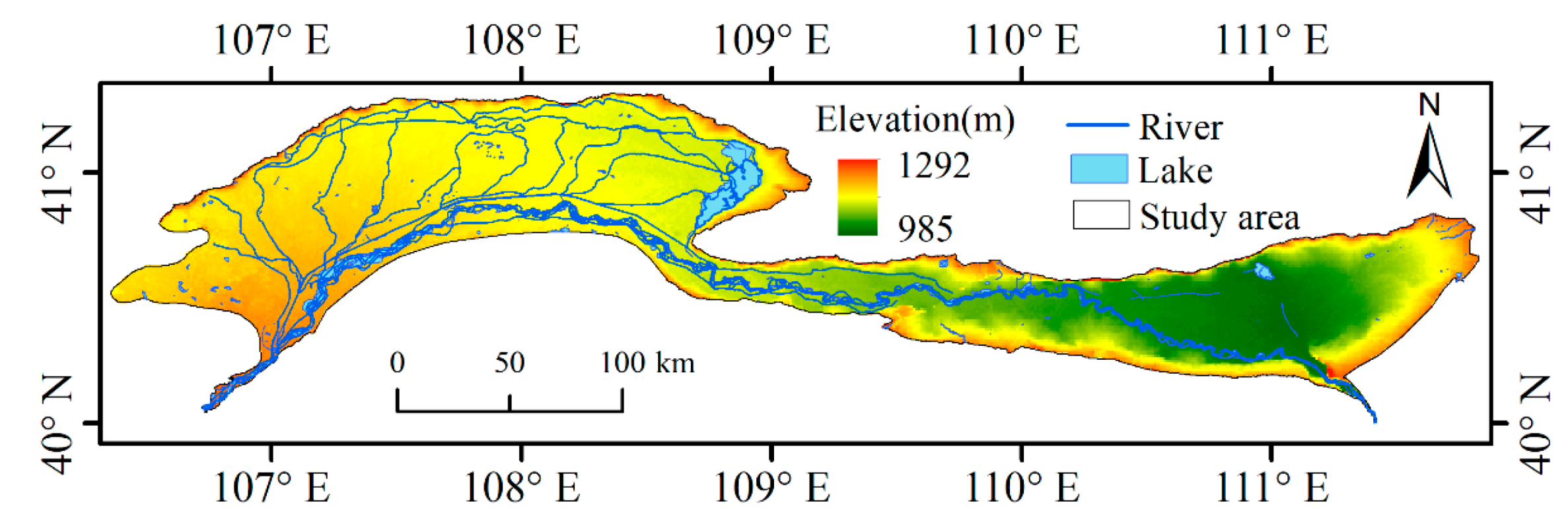
2.1. Study Area
2.2. Data Sources
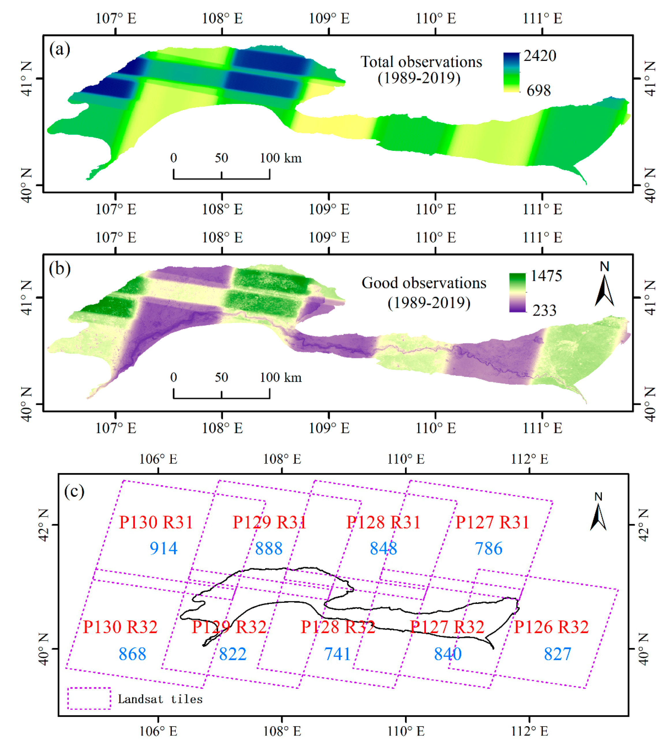
2.2.1. Landsat Data
2.2.2. Climate Data
2.2.3. Sentinel-2 Multispectral Instruments (MSI) Images Data
2.2.4. Globeland 30 Data
3. Research Methods of Surface Water
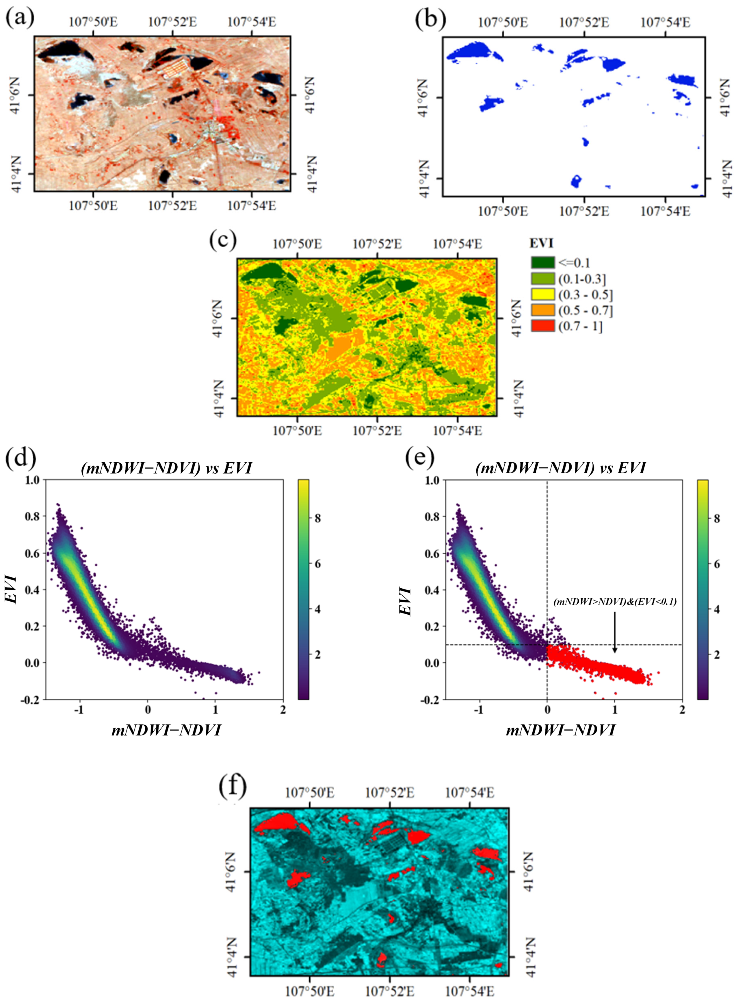
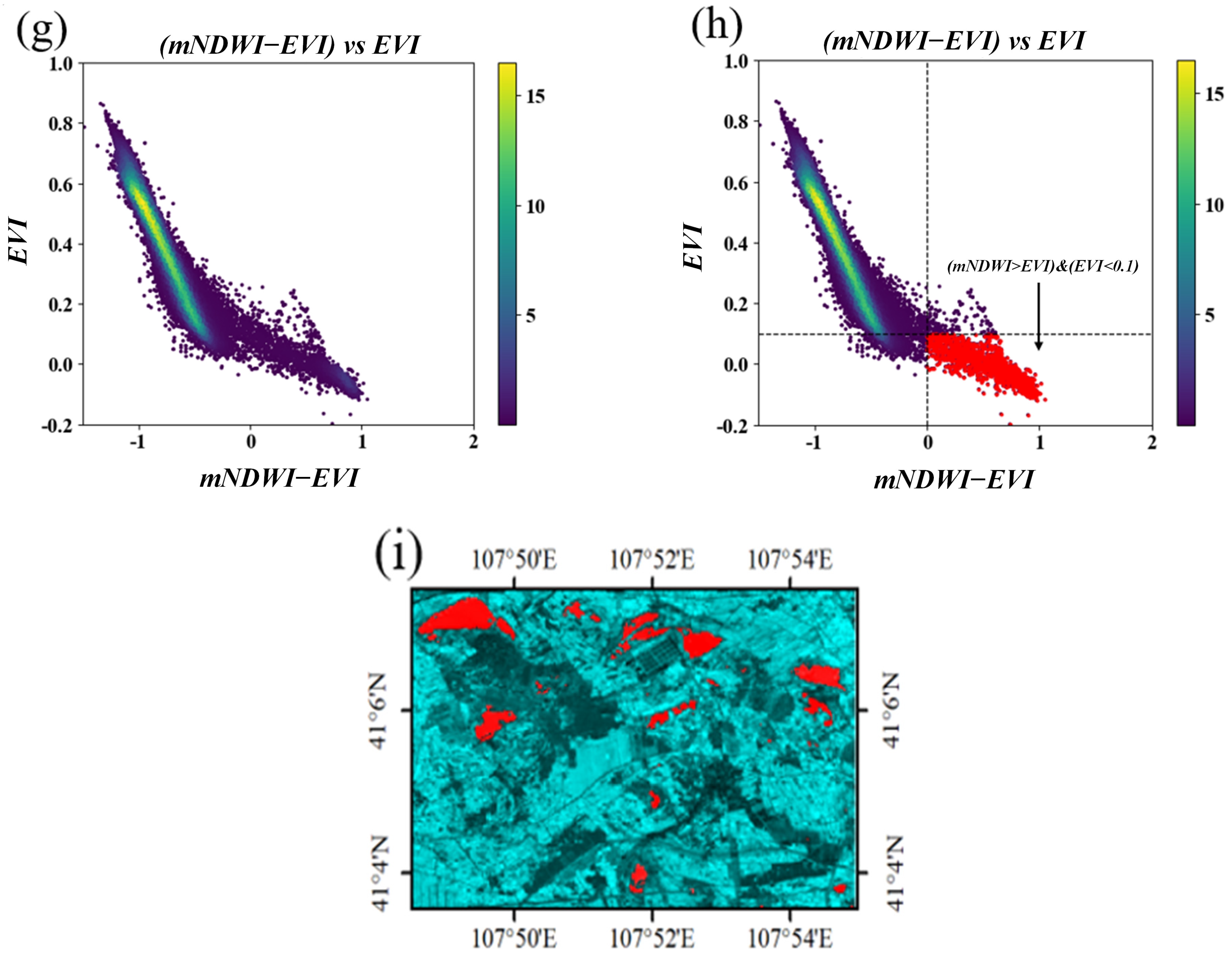
3.1. Surface Water Extraction Algorithm
3.2. Calculation Method of Maximum, Seasonal, Permanent, and Annual Average Water Body
3.3. Surface Water Area and Dynamic Degree
3.3.1. Surface Water Area
3.3.2. Dynamic Degree of Surface Water
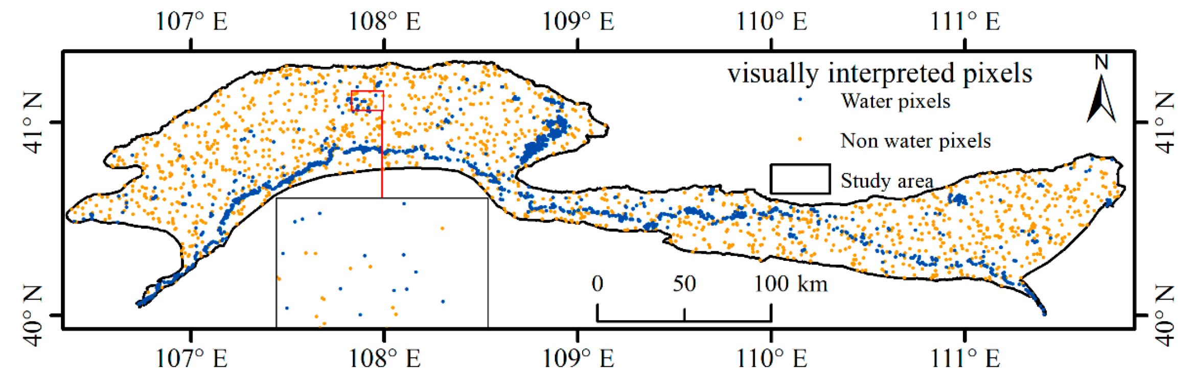
3.4. Accuracy Evaluation Method
4. Result
4.1. Accuracy of Water Body Mapping
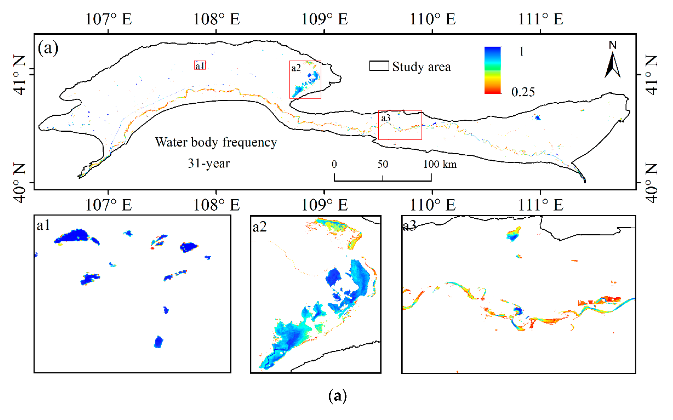
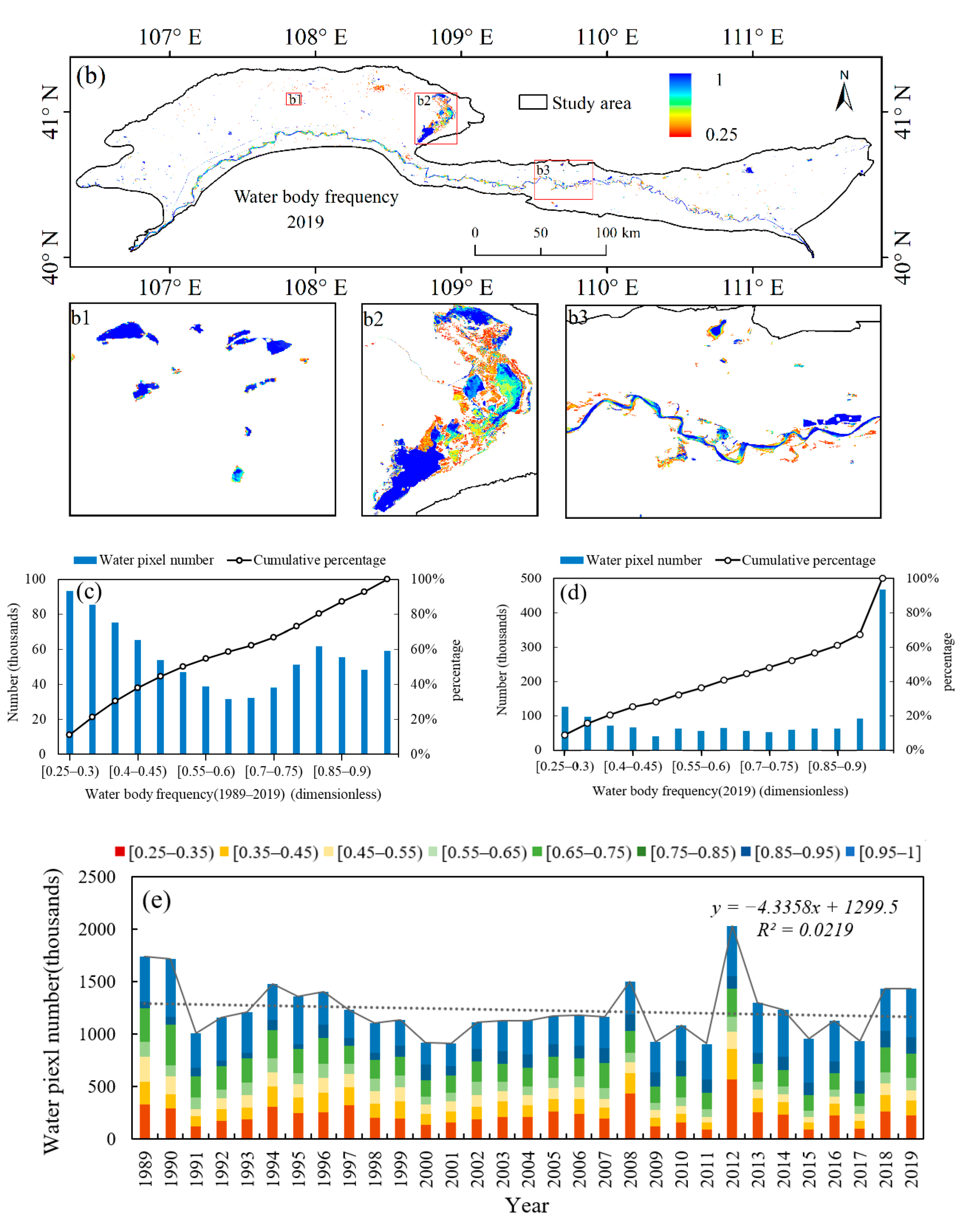
4.2. Spatial Distribution of Surface Water
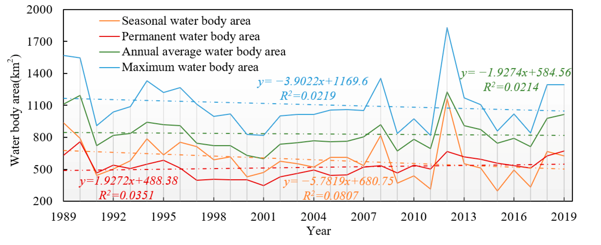
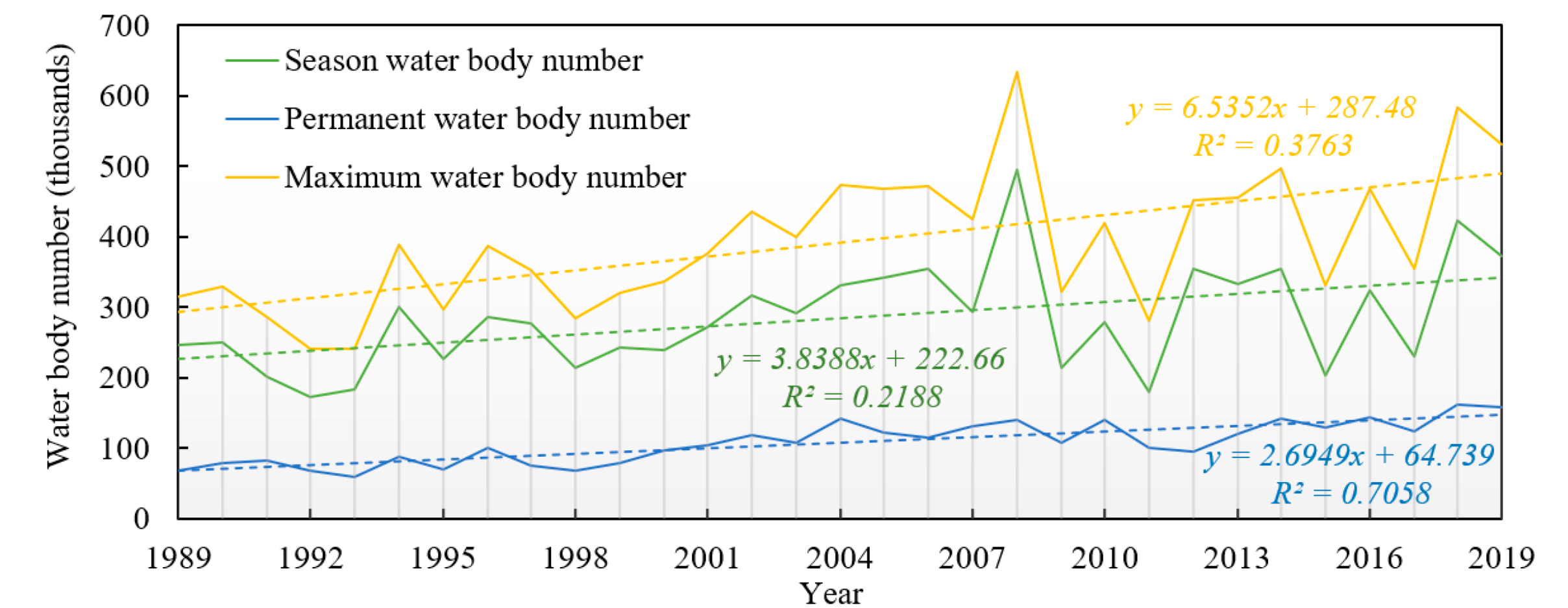
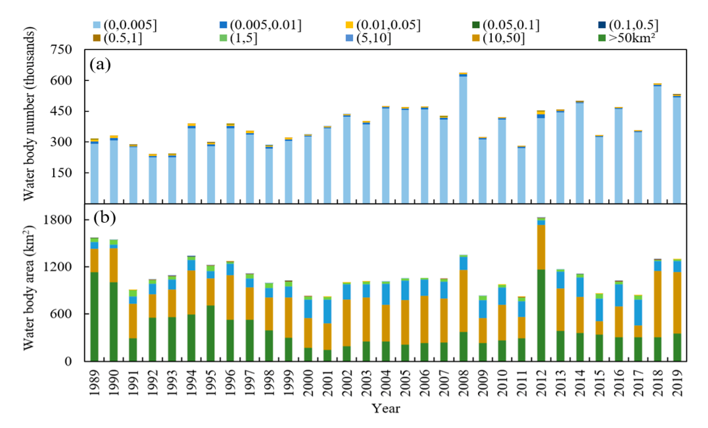
4.3. Temporal Distribution of Surface Water
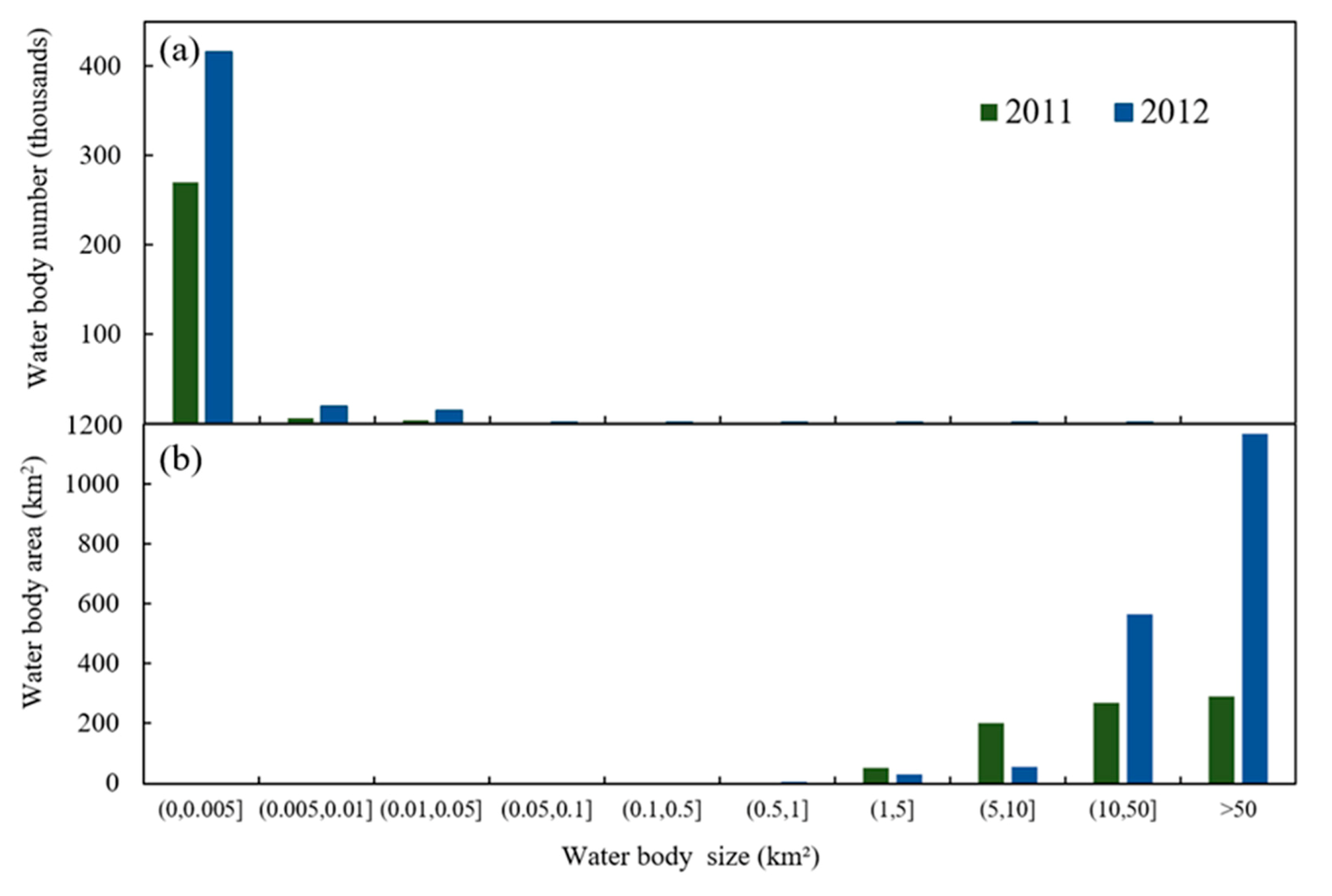
4.4. Influence of Drought and Rainy Years on Surface Water Change
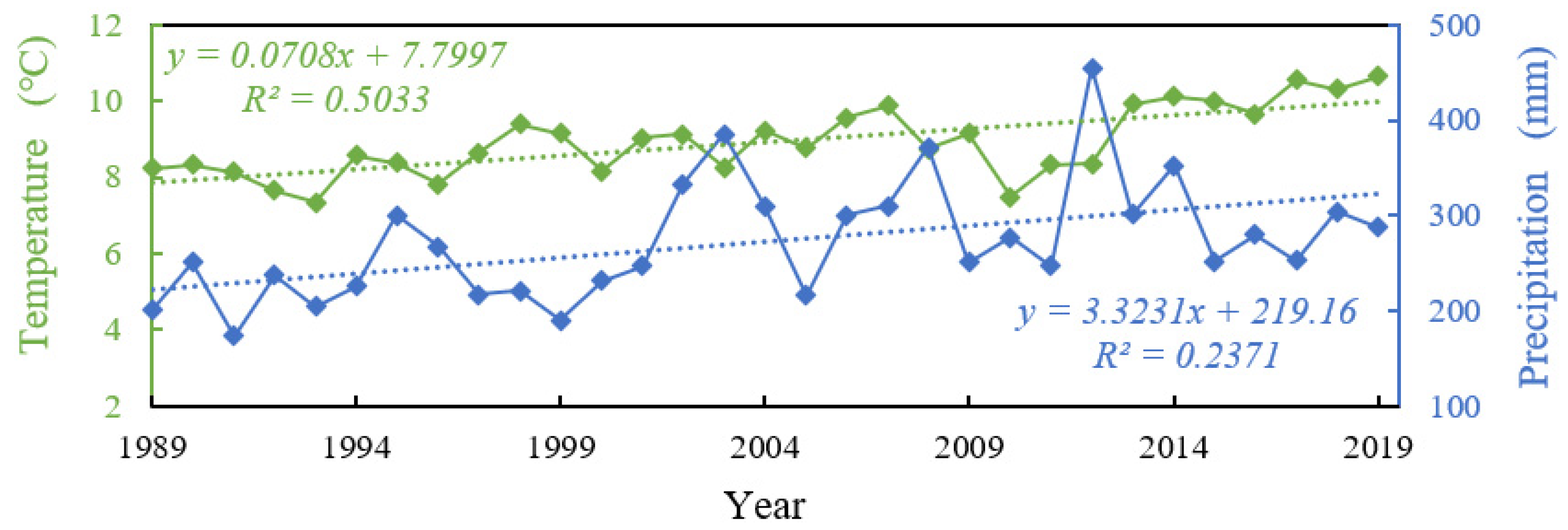
4.5. Influence of Climate Change and Human Activities on Surface Water Change
5. Discussion
5.1. Comparison with the JRC Dataset
5.2. Research Uncertainty
6. Conclusions
Supplementary Materials
Author Contributions
Funding
Conflicts of Interest
References
- Liu, J.; Yang, H.; Gosling, S.N.; Kummu, M.; Florke, M.; Pfister, S.; Hanasaki, N.; Wada, Y.; Zhang, X.; Zheng, C.; et al. Water scarcity assessments in the past, present and future. Earth Future 2017, 5, 545–559. [Google Scholar] [CrossRef] [PubMed]
- Aherne, J.; Larssen, T.; Cosby, B.J.; Dillon, P.J. Climate variability and forecasting surface water recovery from acidification: Modelling drought-induced sulphate release from wetlands. Sci. Total Environ. 2006, 365, 186–199. [Google Scholar] [CrossRef]
- Ferguson, I.M.; Maxwell, R.M. Human impacts on terrestrial hydrology: Climate change versus pumping and irrigation. Environ. Res. Lett. 2012, 7, 0044022. [Google Scholar] [CrossRef] [Green Version]
- Mueller, N.; Lewis, A.; Roberts, D.; Ring, S.; Melrose, R.; Sixsmith, J.; Lymburner, L.; McIntyre, A.; Tan, P.; Curnow, S.; et al. Water observations from space: Mapping surface water from 25 years of Landsat imagery across Australia. Remote Sens. Environ. 2016, 174, 341–352. [Google Scholar] [CrossRef] [Green Version]
- Tulbure, M.G.; Broich, M. Spatiotemporal dynamic of surface water bodies using Landsat time-series data from 1999 to 2011. ISPRS J. Photogramm. Remote Sens. 2013, 79, 44–52. [Google Scholar] [CrossRef]
- Yin, Y.Y.; Tang, Q.H.; Liu, X.C.; Zhang, X.J. Water scarcity under various socio-economic pathways and its potential effects on food production in the Yellow River basin. Hydrol. Earth Syst. Sci. 2017, 21, 791–804. [Google Scholar] [CrossRef] [Green Version]
- Song, C.; Huang, B.; Ke, L. Modeling and analysis of lake water storage changes on the Tibetan Plateau using multi-mission satellite data. Remote Sens. Environ. 2013, 135, 25–35. [Google Scholar] [CrossRef]
- Hall, J.W.; Grey, D.; Garrick, D.; Fung, F.; Brown, C.; Dadson, S.J.; Sadoff, C.W. Coping with the curse of freshwater variability. Science 2014, 346, 429–430. [Google Scholar] [CrossRef]
- Tulbure, M.G.; Broich, M.; Stehman, S.V.; Kommareddy, A. Surface water extent dynamics from three decades of seasonally continuous Landsat time series at subcontinental scale in a semi-arid region. Remote Sens. Environ. 2016, 178, 142–157. [Google Scholar] [CrossRef]
- Zurqani, H.A.; Post, C.J.; Mikhailova, E.A.; Schlautman, M.A.; Sharp, J.L. Geospatial analysis of land use change in the Savannah River Basin using Google Earth Engine. Int. J. Appl. Earth Obs. Geoinf. 2018, 69, 175–185. [Google Scholar] [CrossRef]
- Holben, B.N. Characteristics of maximum-value composite images from temporal AVHRR data. Int. J. Remote Sens. 2007, 7, 1417–1434. [Google Scholar] [CrossRef]
- Li, S.; Sun, D.; Goldberg, M.; Stefanidis, A. Derivation of 30-m-resolution water maps from TERRA/MODIS and SRTM. Remote Sens. Environ. 2013, 134, 417–430. [Google Scholar] [CrossRef]
- Feng, L.; Hou, X.; Zheng, Y. Monitoring and understanding the water transparency changes of fifty large lakes on the Yangtze Plain based on long-term MODIS observations. Remote Sens. Environ. 2019, 221, 675–686. [Google Scholar] [CrossRef]
- Chen, L.; Michishita, R.; Xu, B. Abrupt spatiotemporal land and water changes and their potential drivers in Poyang Lake, 2000–2012. ISPRS J. Photogramm. Remote Sens. 2014, 98, 85–93. [Google Scholar] [CrossRef]
- Chen, B.; Chen, L.; Huang, B.; Michishita, R.; Xu, B. Dynamic monitoring of the Poyang Lake wetland by integrating Landsat and MODIS observations. ISPRS J. Photogramm. Remote Sens. 2018, 139, 75–87. [Google Scholar] [CrossRef]
- Harvey, K.R.; Hill, G.J.E. Vegetation mapping of a tropical freshwater swamp in the Northern Territory, Australia: A comparison of aerial photography, Landsat TM and SPOT satellite imagery. Int. J. Remote Sens. 2001, 22, 2911–2925. [Google Scholar] [CrossRef]
- Li, S.; Sun, D.; Goldberg, M.D.; Sjoberg, B.; Santek, D.; Hoffman, J.P.; DeWeese, M.; Restrepo, P.; Lindsey, S.; Holloway, E. Automatic near real-time flood detection using Suomi-NPP/VIIRS data. Remote Sens. Environ. 2018, 204, 672–689. [Google Scholar] [CrossRef]
- Liao, A.; Chen, L.; Chen, J.; He, C.; Cao, X.; Chen, J.; Peng, S.; Sun, F.; Gong, P. High-resolution remote sensing mapping of global land water. Sci. China Earth Sci. 2014, 57, 2305–2316. [Google Scholar] [CrossRef]
- Feng, M.; Sexton, J.O.; Channan, S.; Townshend, J.R. A global, high-resolution (30-m) inland water body dataset for 2000: First results of a topographic–spectral classification algorithm. Int. J. Digit. Earth. 2015, 9, 113–133. [Google Scholar] [CrossRef] [Green Version]
- Carroll, M.; Wooten, M.; DiMiceli, C.; Sohlberg, R.; Kelly, M. Quantifying Surface Water Dynamics at 30 Meter Spatial Resolution in the North American High Northern Latitudes 1991–2011. Remote Sens. 2016, 8, 622. [Google Scholar] [CrossRef] [Green Version]
- Pekel, J.F.; Cottam, A.; Gorelick, N.; Belward, A.S. High-resolution mapping of global surface water and its long-term changes. Nature 2016, 540, 418–422. [Google Scholar] [CrossRef]
- Sheng, Y.; Song, C.; Wang, J.; Lyons, E.A.; Knox, B.R.; Cox, J.S.; Gao, F. Representative lake water extent mapping at continental scales using multi-temporal Landsat-8 imagery. Remote Sens. Environ. 2016, 185, 129–141. [Google Scholar] [CrossRef] [Green Version]
- Zou, Z.; Dong, J.; Menarguez, M.A.; Xiao, X.; Qin, Y.; Doughty, R.B.; Hooker, K.V.; David Hambright, K. Continued decrease of open surface water body area in Oklahoma during 1984–2015. Sci. Total. Environ. 2017, 595, 451–460. [Google Scholar] [CrossRef]
- Wang, X.; Xiao, X.; Zou, Z.; Hou, L.; Qin, Y.; Dong, J.; Doughty, R.B.; Chen, B.; Zhang, X.; Chen, Y.; et al. Mapping coastal wetlands of China using time series Landsat images in 2018 and Google Earth Engine. ISPRS J. Photogramm. Remote Sens. 2020, 163, 312–326. [Google Scholar] [CrossRef] [PubMed]
- Wang, X.; Xiao, X.; Zou, Z.; Chen, B.; Ma, J.; Dong, J.; Doughty, R.B.; Zhong, Q.; Qin, Y.; Dai, S.; et al. Tracking annual changes of coastal tidal flats in China during 1986–2016 through analyses of Landsat images with Google Earth Engine. Remote Sens. Environ. 2020, 238, 110987. [Google Scholar] [CrossRef]
- Du, Y.; Zhang, Y.; Ling, F.; Wang, Q.; Li, W.; Li, X. Water Bodies’ Mapping from Sentinel-2 Imagery with Modified Normalized Difference Water Index at 10 m Spatial Resolution Produced by Sharpening the SWIR Band. Remote Sens. 2016, 8, 354. [Google Scholar] [CrossRef] [Green Version]
- Yang, X.; Zhao, S.; Qin, X.; Zhao, N.; Liang, L. Mapping of Urban Surface Water Bodies from Sentinel-2 MSI Imagery at 10 m Resolution via NDWI-Based Image Sharpening. Remote Sens. 2017, 9, 596. [Google Scholar] [CrossRef] [Green Version]
- Hansen, M.C.; Egorov, A.; Potapov, P.V.; Stehman, S.V.; Tyukavina, A.; Turubanova, S.A.; Roy, D.P.; Goetz, S.J.; Loveland, T.R.; Ju, J.; et al. Monitoring conterminous United States (CONUS) land cover change with Web-Enabled Landsat Data (WELD). Remote Sens. Environ. 2014, 140, 466–484. [Google Scholar] [CrossRef] [Green Version]
- Yamazaki, D.; Trigg, M.A.; Ikeshima, D. Development of a global ~90m water body map using multi-temporal Landsat images. Remote Sens. Environ. 2015, 171, 337–351. [Google Scholar] [CrossRef]
- Hou, X.; Feng, L.; Duan, H.; Chen, X.; Sun, D.; Shi, K. Fifteen-year monitoring of the turbidity dynamics in large lakes and reservoirs in the middle and lower basin of the Yangtze River, China. Remote Sens. Environ. 2017, 190, 107–121. [Google Scholar] [CrossRef]
- Feng, L.; Hu, C.; Chen, X.; Li, R. Satellite observations make it possible to estimate Poyang Lake’s water budget. Environ Res. Lett. 2011, 6, 044023. [Google Scholar] [CrossRef]
- Homer, C.; Dewitz, J.; Yang, L.; Jin, S.; Danielson, P.; Xian, G.; Coulston, J.; Herold, N.; Wickham, J.; Megown, K. Completion of the 2011 National Land Cover Database for the Conterminous United States—Representing a Decade of Land Cover Change Information. Photogramm. Eng. Remote Sens. 2015, 81, 345–354. [Google Scholar]
- Gorelick, N.; Hancher, M.; Dixon, M.; Ilyushchenko, S.; Thau, D.; Moore, R. Google Earth Engine: Planetary-scale geospatial analysis for everyone. Remote Sens. Environ. 2017, 202, 18–27. [Google Scholar] [CrossRef]
- Dong, J.; Xiao, X.; Menarguez, M.A.; Zhang, G.; Qin, Y.; Thau, D.; Biradar, C.; Moore, B. Mapping paddy rice planting area in northeastern Asia with Landsat 8 images, phenology-based algorithm and Google Earth Engine. Remote Sens. Environ. 2016, 185, 142–154. [Google Scholar] [CrossRef] [Green Version]
- Shelestov, A.; Lavreniuk, M.; Kussul, N.; Novikov, A.; Skakun, S. Exploring Google Earth Engine Platform for Big Data Processing: Classification of Multi-Temporal Satellite Imagery for Crop Mapping. Front. Earth Sci. 2017, 5, 17. [Google Scholar] [CrossRef] [Green Version]
- Xiong, J.; Thenkabail, P.S.; Gumma, M.K.; Teluguntla, P.; Poehnelt, J.; Congalton, R.G.; Yadav, K.; Thau, D. Automated cropland mapping of continental Africa using Google Earth Engine cloud computing. ISPRS J. Photogramm. Remote Sens. 2017, 126, 225–244. [Google Scholar] [CrossRef] [Green Version]
- Zhou, Y.; Dong, J. Review on monitoring open surface water body using remote sensing. J. Geogr. Inf. Sci. 2019, 21, 1768–1778. [Google Scholar]
- Feng, Q.; Liu, J.; Gong, J. Urban Flood Mapping Based on Unmanned Aerial Vehicle Remote Sensing and Random Forest Classifier—A Case of Yuyao, China. Water 2015, 7, 1437–1455. [Google Scholar] [CrossRef]
- Ko, B.; Kim, H.H.; Nam, J.Y. Classification of Potential Water Bodies Using Landsat 8 OLI and a Combination of Two Boosted Random Forest Classifiers. Sensors 2015, 15, 13763–13777. [Google Scholar] [CrossRef] [Green Version]
- Acharya, T.D.; Lee, D.H.; Yang, I.T.; Lee, J.K. Identification of Water Bodies in a Landsat 8 OLI Image Using a J48 Decision Tree. Sensors 2016, 16, 1075. [Google Scholar] [CrossRef] [Green Version]
- Hinton, G.E.; Salakhutdinov, R.R. Reducing the Dimensionality of Data with Neural Networks. Science 2006, 313, 504–507. [Google Scholar] [CrossRef] [PubMed] [Green Version]
- Li, W.; Du, Z.; Ling, F.; Zhou, D.; Wang, H.; Gui, Y.; Sun, B.; Zhang, X. A Comparison of Land Surface Water Mapping Using the Normalized Difference Water Index from TM, ETM+ and ALI. Remote Sens. 2013, 5, 5530–5549. [Google Scholar] [CrossRef] [Green Version]
- Huang, C.; Chen, Y.; Zhang, S.; Wu, J. Detecting, Extracting, and Monitoring Surface Water from Space Using Optical Sensors: A Review. Rev. Geophys. 2018, 56, 333–360. [Google Scholar] [CrossRef]
- McFeeters, S.K. The use of the Normalized Difference Water Index (NDWI) in the delineation of open water features. Int. J. Remote Sens. 2007, 17, 1425–1432. [Google Scholar] [CrossRef]
- Feyisa, G.L.; Meilby, H.; Fensholt, R.; Proud, S.R. Automated Water Extraction Index: A new technique for surface water mapping using Landsat imagery. Remote Sens. Environ. 2014, 140, 23–35. [Google Scholar] [CrossRef]
- Fisher, A.; Flood, N.; Danaher, T. Comparing Landsat water index methods for automated water classification in eastern Australia. Remote Sens. Environ. 2016, 175, 167–182. [Google Scholar] [CrossRef]
- Chen, B.; Xiao, X.; Li, X.; Pan, L.; Doughty, R.; Ma, J.; Dong, J.; Qin, Y.; Zhao, B.; Wu, Z.; et al. A mangrove forest map of China in 2015: Analysis of time series Landsat 7/8 and Sentinel-1A imagery in Google Earth Engine cloud computing platform. ISPRS J. Photogramm. Remote Sens. 2017, 131, 104–120. [Google Scholar] [CrossRef]
- Mohammadi, A.; Costelloe, J.F.; Ryu, D. Application of time series of remotely sensed normalized difference water, vegetation and moisture indices in characterizing flood dynamics of large-scale arid zone flood Plains. Remote Sens. Environ. 2017, 190, 70–82. [Google Scholar] [CrossRef]
- Wang, Y.; Ma, J.; Xiao, X.; Wang, X.; Dai, S.; Zhao, B. Long-Term Dynamic of Poyang Lake Surface Water: A Mapping Work Based on the Google Earth Engine Cloud Platform. Remote Sens. 2019, 11, 313. [Google Scholar] [CrossRef] [Green Version]
- Liu, H.; Yin, Y.; Piao, S.; Zhao, F.; Engels, M.; Ciais, P. Disappearing lakes in semiarid Northern China: Drivers and environmental impact. Environ Sci. Technol. 2013, 47, 12107–12114. [Google Scholar] [CrossRef]
- Jin, S.; Yang, L.; Danielson, P.; Homer, C.; Fry, J.; Xian, G. A comprehensive change detection method for updating the National Land Cover Database to circa 2011. Remote Sens. Environ. 2013, 132, 159–175. [Google Scholar] [CrossRef] [Green Version]
- Chen, F.; Zhang, M.; Tian, B.; Li, Z. Extraction of Glacial Lake Outlines in Tibet Plateau Using Landsat 8 Imagery and Google Earth Engine. IEEE J. Sel. Top Appl. Earth Obs. Remote Sens. 2017, 10, 4002–4009. [Google Scholar] [CrossRef]
- Nyland, E.K.; Gunn, G.E.; Shiklomanov, N.I.; Engstrom, N.R.; Streletskiy, D.A. Land Cover Change in the Lower Yenisei River Using Dense Stacking of Landsat Imagery in Google Earth Engine. Remote Sens. 2018, 10, 1226. [Google Scholar] [CrossRef] [Green Version]
- Zou, Z.; Xiao, X.; Dong, J.; Qin, Y.; Doughty, R.B.; Menarguez, M.A.; Zhang, G.; Wang, J. Divergent trends of open-surface water body area in the contiguous United States from 1984 to 2016. Proc. Natl. Acad. Sci. USA 2018, 115, 3810–3815. [Google Scholar] [CrossRef] [PubMed] [Green Version]
- Xia, H.; Zhao, J.; Qin, Y.; Yang, J.; Cui, Y.; Song, H.; Ma, L.; Jin, N.; Meng, Q. Changes in Water Surface Area during 1989–2017 in the Huai River Basin using Landsat Data and Google Earth Engine. Remote Sens. 2019, 11, 1824. [Google Scholar] [CrossRef] [Green Version]
- Wang, X.; Xiao, X.; Zou, Z.; Dong, J.; Qin, Y.; Doughty, R.B.; Menarguez, M.A.; Chen, B.; Wang, J.; Ye, H.; et al. Gainers and losers of surface and terrestrial water resources in China during 1989–2016. Nat. Commun. 2020, 11, 3471. [Google Scholar] [CrossRef] [PubMed]
- Dwyer, J.L.; Roy, D.P.; Sauer, B.; Jenkerson, C.B.; Zhang, H.K.; Lymburner, L. Analysis ready data: Enabling analysis of the Landsat archive. Remote Sens. 2018, 10, 1363. [Google Scholar]
- Wulder, M.A.; White, J.C.; Loveland, T.R.; Woodcock, C.E.; Belward, A.S.; Cohen, W.B.; Fosnight, E.A.; Shaw, J.; Masek, J.G.; Roy, D.P. The global Landsat archive: Status, consolidation, and direction. Remote Sens. Environ. 2016, 185, 271–283. [Google Scholar] [CrossRef] [Green Version]
- Zhou, Y.; Dong, J.; Xiao, X.; Liu, R.; Zou, Z.; Zhao, G.; Ge, Q. Continuous monitoring of lake dynamics on the Mongolian Plateau using all available Landsat imagery and Google Earth Engine. Sci. Total Environ. 2019, 689, 366–380. [Google Scholar] [CrossRef]
- Foga, S.; Scaramuzza, P.L.; Guo, S.; Zhu, Z.; Dilley, R.D.; Beckmann, T.; Schmidt, G.L.; Dwyer, J.L.; Joseph Hughes, M.; Laue, B. Cloud detection algorithm comparison and validation for operational Landsat data products. Remote Sens. Environ. 2017, 194, 379–390. [Google Scholar] [CrossRef] [Green Version]
- Rodell, M.; Houser, P.R.; Jambor, U.E.A.; Gottschalck, J.; Mitchell, K.; Meng, C.J.; Arsenault, K.; Cosgrove, B.; Radakovich, J.; Bosilovich, M.; et al. The Global Land Data Assimilation System. Bam. Meteorol. Soc. 2004, 85, 381–394. [Google Scholar] [CrossRef] [Green Version]
- Jun, C.; Ban, Y.; Li, S. Open access to Earth land-cover map. Nature 2014, 514, 434. [Google Scholar] [CrossRef] [Green Version]
- Tao, S.; Fang, J.; Zhao, X.; Zhao, S.; Shen, H.; Hu, H.; Tang, Z.; Wang, Z.; Guo, Q. Rapid loss of lakes on the Mongolian Plateau. Proc. Indian Natl. Sci. 2015, 112, 2281–2286. [Google Scholar] [CrossRef] [PubMed] [Green Version]
- Xu, H. Modification of normalised difference water index (NDWI) to enhance open water features in remotely sensed imagery. Int. J. Remote Sens. 2006, 27, 3025–3033. [Google Scholar] [CrossRef]
- Lei, J.I.; Zhang, L.I.; Wylie, B. Analysis of Dynamic Thresholds for the Normalized Difference Water Index. Photogramm. Eng. Remote Sens. 2009, 75, 1307–1317. [Google Scholar]
- Verpoorter, C.; Kutser, T.; Tranvik, L. Automated mapping of water bodies using Landsat multispectral data. Limnol. Oceanogr. Meth. 2012, 10, 1037–1050. [Google Scholar] [CrossRef]
- Santoro, M.; Wegmueller, U.; Lamarche, C.; Bontemps, S.; Defoumy, P.; Arino, O. Strengths and weaknesses of multi-year Envisat ASAR backscatter measurements to map permanent open water bodies at global scale. Remote Sens. Environ. 2015, 171, 185–201. [Google Scholar] [CrossRef]
- Su, K.; Wei, D.Z.; Lin, W.X. Evaluation of ecosystem services value and its implications for policy making in China—A case study of Fujian province. Ecol. Indic. 2020, 108, 105752. [Google Scholar] [CrossRef]
- Yigzaw, W.; Hossain, F. Water sustainability of large cities in the United States from the perspectives of population increase, anthropogenic activities, and climate change. Earth Future 2016, 4, 603–617. [Google Scholar] [CrossRef]
- Xia, H.; Qin, Y.; Feng, G.; Meng, Q.; Cui, Y.; Song, H.; Ouyang, Y.; Liu, G. Forest Phenology Dynamics to Climate Change and Topography in a Geographic and Climate Transition Zone: The Qinling Mountains in Central China. Forests 2019, 10, 1007. [Google Scholar] [CrossRef] [Green Version]
- Xia, H.; Zhao, W.; Li, A.; Bian, J.; Zhang, Z. Subpixel Inundation Mapping Using Landsat-8 OLI and UAV Data for a Wetland Region on the Zoige Plateau, China. Remote Sens. 2017, 9, 31. [Google Scholar] [CrossRef] [Green Version]
- Zhai, K.; Wu, X.; Qin, Y.; Du, P. Comparison of surface water extraction performances of different classic water indices using OLI and TM imageries in different situations. Geo. Spat. Inf. Sci. 2015, 18, 32–42. [Google Scholar] [CrossRef]
- Zhou, Y.; Dong, J.; Xiao, X.; Xiao, T.; Yang, Z.; Zhao, G.; Zou, Z.; Qin, Y. Open Surface Water Mapping Algorithms: A Comparison of Water-Related Spectral Indices and Sensors. Water 2017, 9, 256. [Google Scholar] [CrossRef]


| Sentinel-2 MSI | ||||
|---|---|---|---|---|
| Water Body Map (2019) | Water | No Water | Total | User Accuracy (%) |
| Water | 952 | 55 | 1007 | 94.54% |
| No-Water | 69 | 1924 | 1993 | 96.54% |
| Total | 1021 | 1979 | 3000 | Overall Accuracy = 95.9% |
| Producer Accuracy (%) | 93.24% | 97.22% | Kappa Coefficient = 0.91 | |
| Year | Number | Number Change | Dynamic Index | Overall Dynamic Change |
|---|---|---|---|---|
| 1989–1994 | 300,169 | - | - | 45.75% |
| 1995–1999 | 328,336 | 28,167 | 9.38% | |
| 2000–2004 | 403,831 | 75,495 | 22.99% | |
| 2005–2009 | 464,241 | 6041 | 14.96% | |
| 2010–2014 | 420,587 | −43,654 | −9.4% | |
| 2015–2019 | 453,496 | 32,909 | 7.82% |
| Year | Area(km2) | Area Change | Dynamic Index | Overall Dynamic Change |
|---|---|---|---|---|
| 1989–1994 | 1246.471 | - | - | −12.09% |
| 1995–1999 | 1122.563 | −123.908 | −9.94% | |
| 2000–2004 | 935.649 | −186.914 | −16.65% | |
| 2005–2009 | 1070.912 | 135.263 | 14.46% | |
| 2010–2014 | 1178.781 | 107.869 | 10.07% | |
| 2015–2019 | 1060.578 | −118.203 | −10.03% |
| Maximum | Seasonal | Permanent | ||||
|---|---|---|---|---|---|---|
| Variables | Area | Number | Area | Number | Area | Number |
| Coef. | Coef. | Coef. | Coef. | Coef. | Coef. | |
| AP | 2.899 | 0.976 | 2.016 | 0.752 | 0.785 | 0.225 |
| AT | ||||||
| Irrigation | −8.155 | −6.269 | −1.864 | |||
| Constant | 1164.863 | 126.219 | 674.052 | 79.172 | 489.671 | 46.479 |
| Model summary | ||||||
| R2 | 0.51 | 0.391 | 0.463 | 0.392 | 0.245 | 0.23 |
| SEE | 175 | 76 | 142 | 59 | 81 | 26 |
| F | 14.065 | 18.627 | 11.64 | 18.665 | 4.384 | 8.661 |
| Sig. | 0.000 | 0.000 | 0.000 | 0.000 | 0.022 | 0.006 |
Publisher’s Note: MDPI stays neutral with regard to jurisdictional claims in published maps and institutional affiliations. |
© 2020 by the authors. Licensee MDPI, Basel, Switzerland. This article is an open access article distributed under the terms and conditions of the Creative Commons Attribution (CC BY) license (http://creativecommons.org/licenses/by/4.0/).
Share and Cite
Wang, R.; Xia, H.; Qin, Y.; Niu, W.; Pan, L.; Li, R.; Zhao, X.; Bian, X.; Fu, P. Dynamic Monitoring of Surface Water Area during 1989–2019 in the Hetao Plain Using Landsat Data in Google Earth Engine. Water 2020, 12, 3010. https://0-doi-org.brum.beds.ac.uk/10.3390/w12113010
Wang R, Xia H, Qin Y, Niu W, Pan L, Li R, Zhao X, Bian X, Fu P. Dynamic Monitoring of Surface Water Area during 1989–2019 in the Hetao Plain Using Landsat Data in Google Earth Engine. Water. 2020; 12(11):3010. https://0-doi-org.brum.beds.ac.uk/10.3390/w12113010
Chicago/Turabian StyleWang, Ruimeng, Haoming Xia, Yaochen Qin, Wenhui Niu, Li Pan, Rumeng Li, Xiaoyang Zhao, Xiqing Bian, and Pinde Fu. 2020. "Dynamic Monitoring of Surface Water Area during 1989–2019 in the Hetao Plain Using Landsat Data in Google Earth Engine" Water 12, no. 11: 3010. https://0-doi-org.brum.beds.ac.uk/10.3390/w12113010