
Predicting Maize Transpiration, Water Use and Productivity for Developing Improved Supplemental Irrigation Schedules in Western Uruguay to Cope with Climate Variability


Abstract
:
1. Introduction
2. Materials and Methods
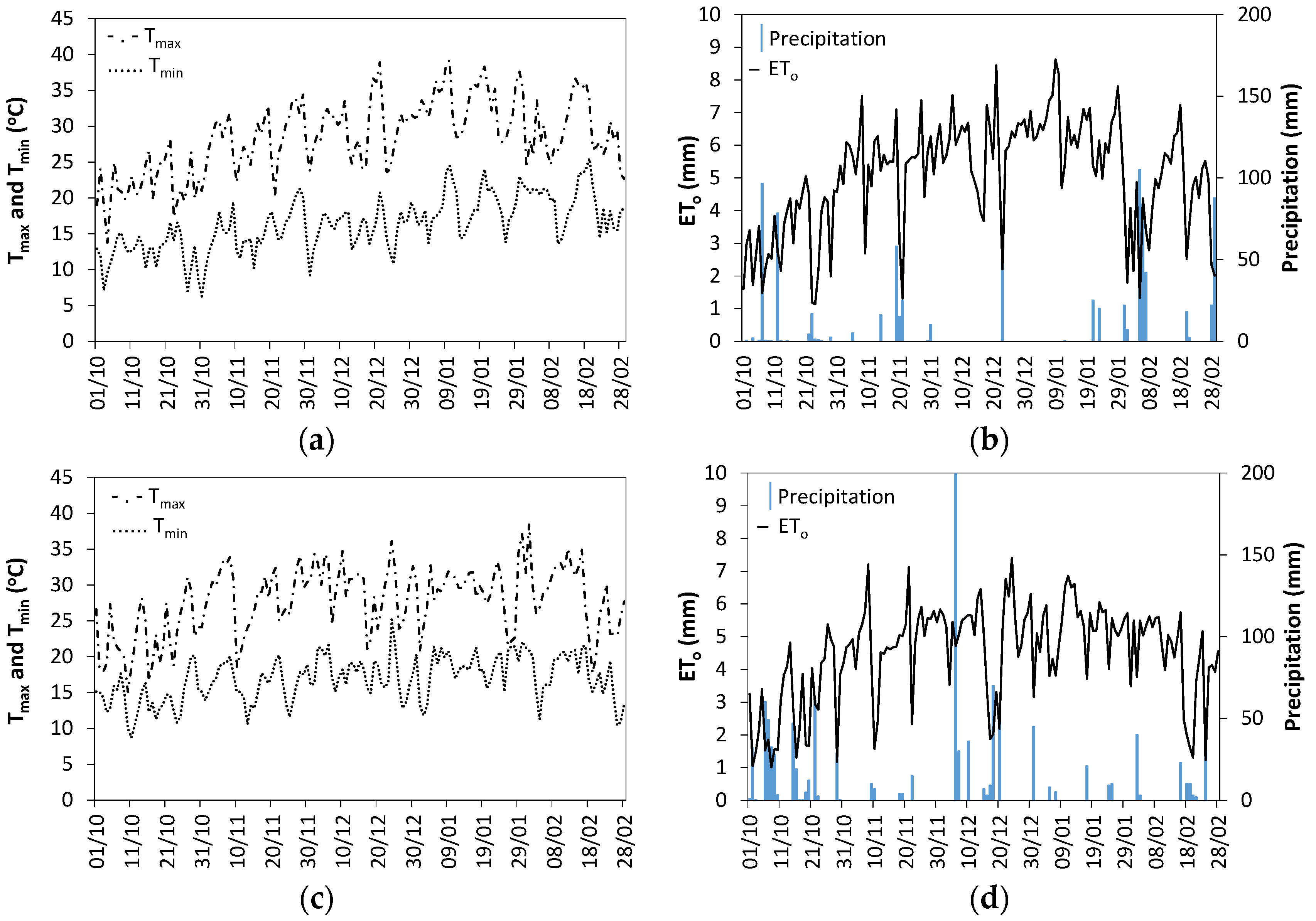
2.1. Site Characterization
- -
- FI, full irrigation, aimed at minimizing water stress in all crop growth stages;
- -
- DIFLO, deficit irrigation from end flowering to the late reproductive stage (1–28 January 2013);
- -
- DIMAT, deficit irrigation during the maturation period (1–10 February 2013);
- -
- DIVEG+REP, deficit irrigation during the vegetative and the reproductive stages (15 November–5 December 2012 and 5–28 January 2013); and
- -
- Rainfed.
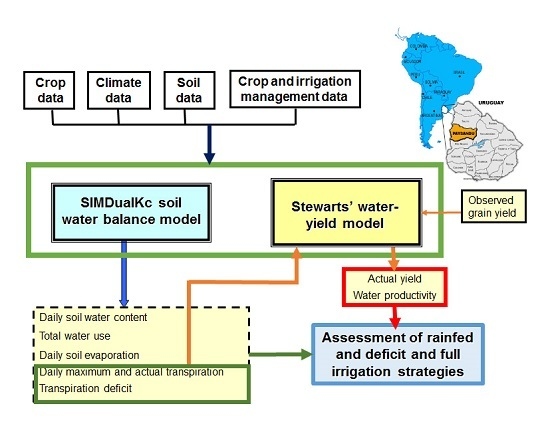
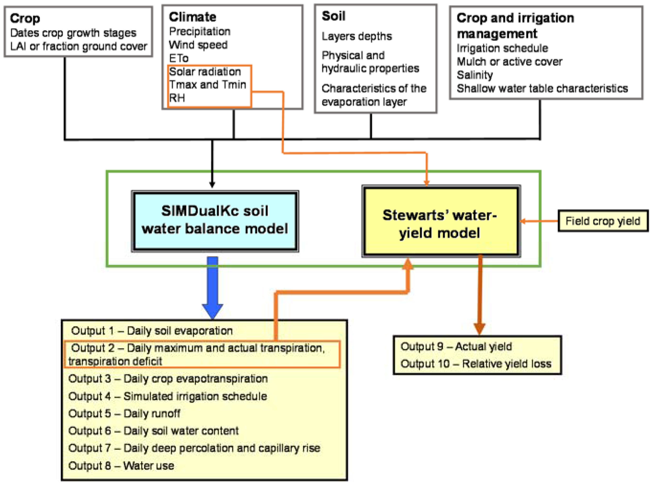
2.2. Modeling
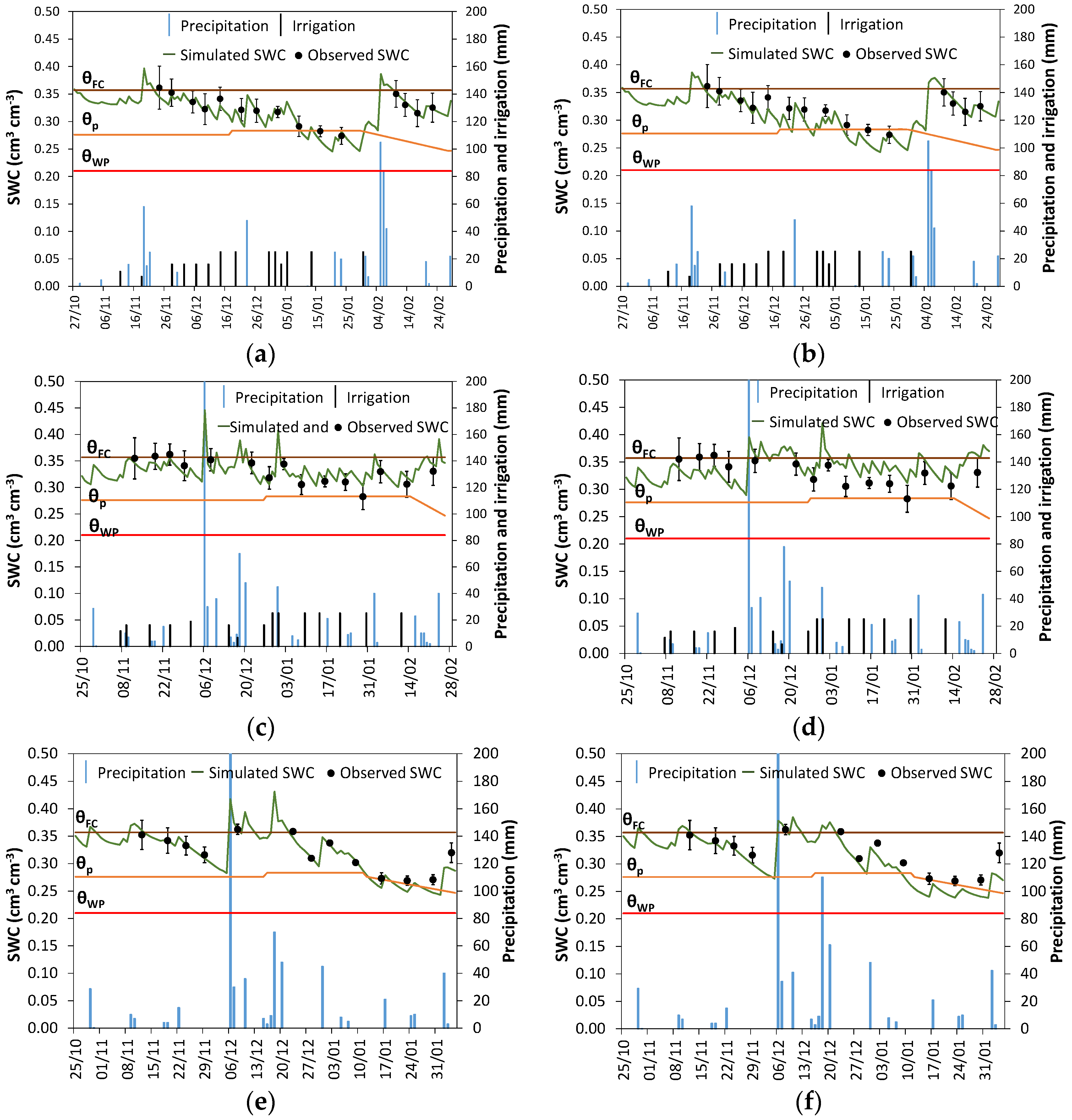
2.3. Calibration and Validation Procedures
- The regression coefficient b0 of a regression forced to the origin (FTO) relating Oi and Pi SWC values, which aim at recognizing how similar were the simulated and observed values, computed as
- The determination coefficient of the ordinary least squares regression of the same variables aimed at assessing the fraction of the variance of observations that was explained by the model.
- The root mean square error (RMSE), which expresses the variance of the residual errors, computed aswhich may vary between 0.0, when a perfect match would occur, and a positive value, which should be smaller than the mean of observations.
- The normalized RMSE (NRMSE), that is defined as the ratio between RMSE and the observations mean , which expedites the comparison of its values for different variables, computed as
- The average relative error (ARE), that expresses the estimation errors as a percentage of observation values
2.4. Generating and Assessing Alternative Supplemental Irrigation Scenarios
- Full irrigation (Full), aimed at preventing water stress, with MAD = p.
- Mild deficit irrigation (Mild): MAD = 1.20 p for the initial period, MAD = 1.30 p for the crop development and the late season periods, and MAD = 1.10 p during mid-season, which includes flowering and yield formation.
- Moderate deficit irrigation (Mod) with MAD = 1.30 p for the initial and crop development periods, MAD = 1.20 p for the mid-season period, and MAD = 1.40 p for the late-season, after grain filling until harvesting.
- Rainfed.
3. Results and Discussion
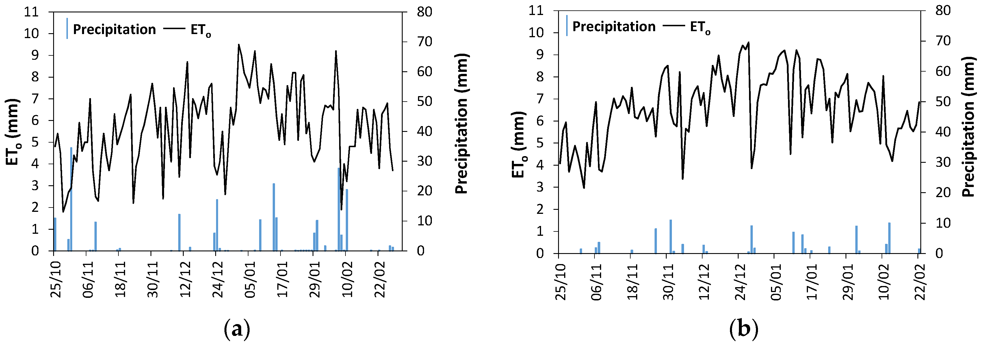
3.1. Soil Water Balance Modeling and Model Parameterization
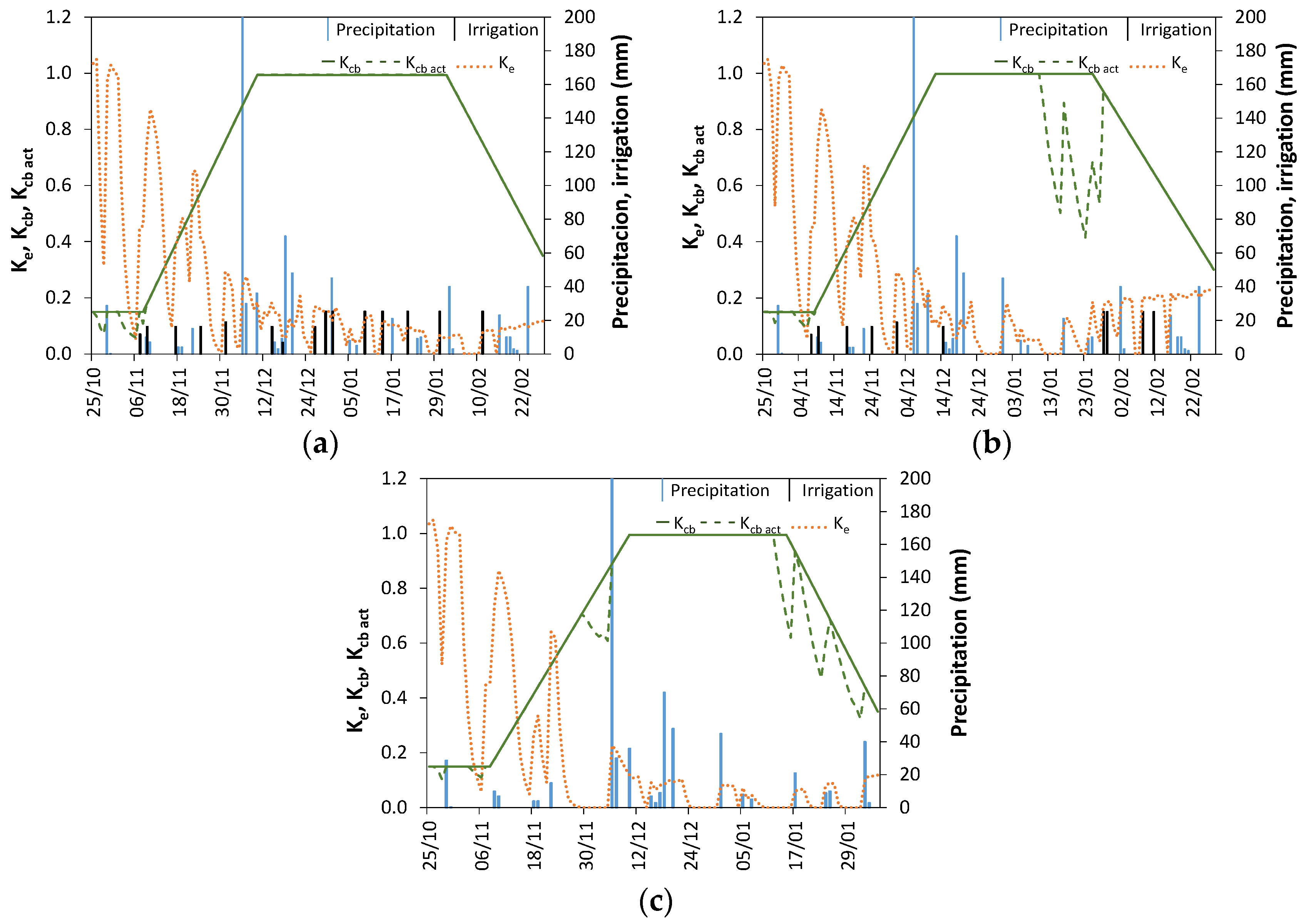
3.2. Crop Coefficients and ET Partitioning
3.3. Water–Yield Relations and Yield Predictions
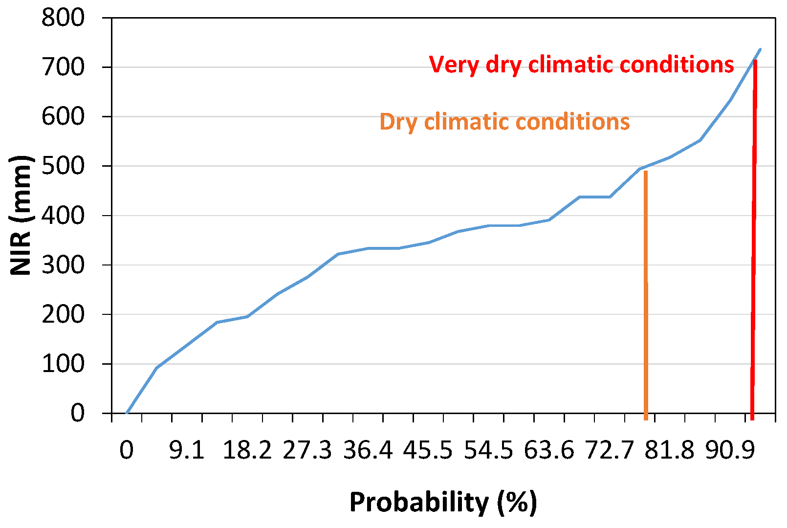
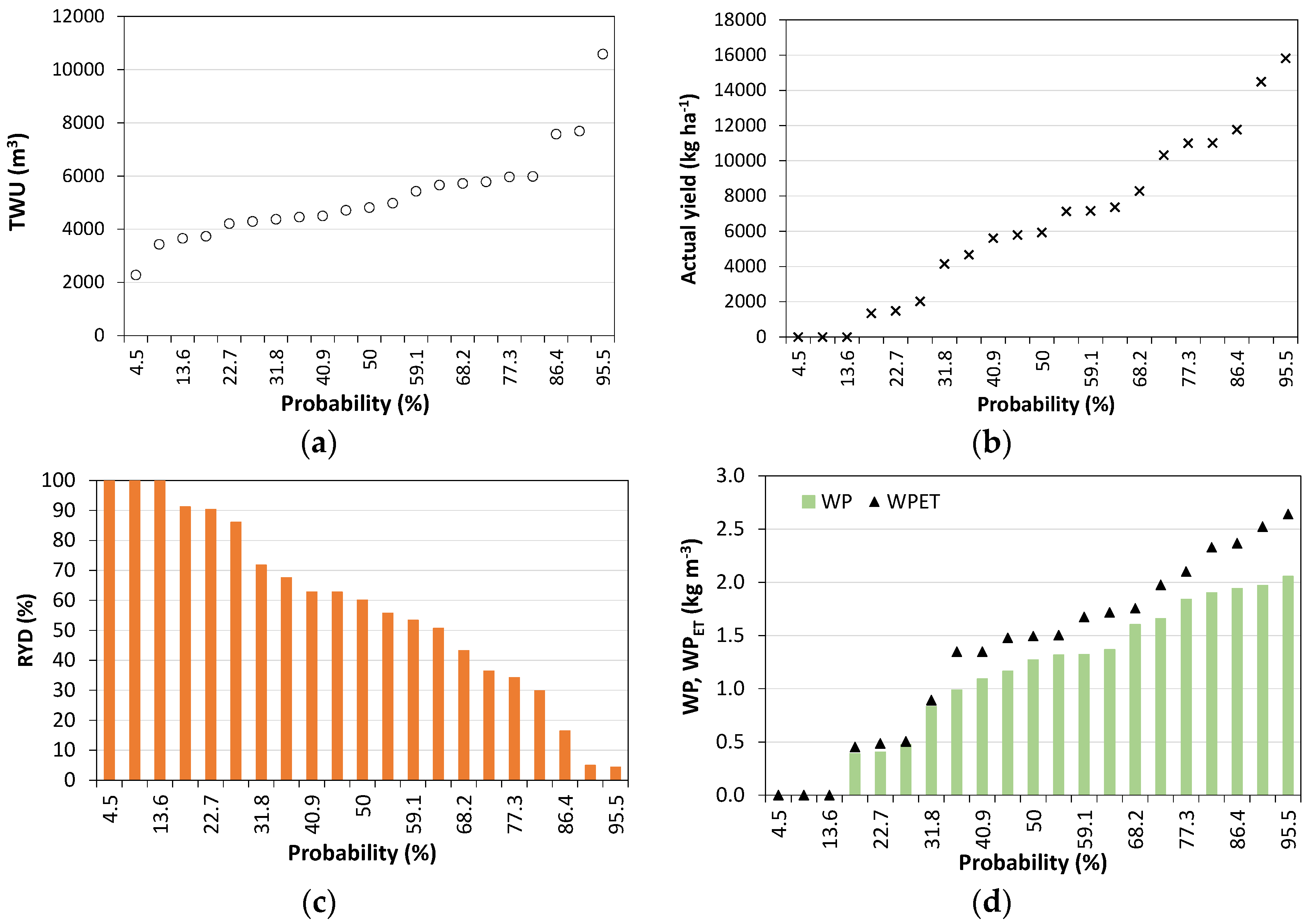
3.4. Assessing Supplemental Irrigation and Rainfed Scenarios under Water Scarcity
4. Conclusions
Acknowledgments
Author Contributions
Conflicts of Interest
References
- Redo, D.J.; Aide, T.M.; Clark, M.L.; Andrade-Núñez, M.J. Impacts of internal and external policies on land change in Uruguay, 2001–2009. Environ. Conserv. 2012, 39, 122–131. [Google Scholar] [CrossRef]
- Giménez, L. Production of corn with water stress at different stages of development. Agrociencia 2012, 16, 92–102. (In Spanish) [Google Scholar]
- Frank, F.C.; Viglizzo, E.F. Water use in rain-fed farming at different scales in the Pampas of Argentina. Agric. Syst. 2012, 109, 35–42. [Google Scholar] [CrossRef]
- García-Préchac, F.; Ernst, O.; Siri-Prieto, G.; Terra, J.A. Integrating no-till into crop-pasture rotations in Uruguay. Soil Till. Res. 2004, 77, 1–13. [Google Scholar] [CrossRef]
- Wingeyer, A.B.; Amado, T.J.C.; Pérez-Bidegain, M.; Studdert, G.A.; Varela, C.H.P.; Garcia, F.O.; Karlen, D.L. Soil quality impacts of current South American agricultural practices. Sustainability 2015, 7, 2213–2242. [Google Scholar] [CrossRef]
- Popova, Z.; Ivanova, M.; Martins, D.; Pereira, L.S.; Doneva, K.; Alexandrov, V.M.; Kercheva, M. Vulnerability of Bulgarian agriculture to drought and climate variability with focus on rainfed maize systems. Nat. Hazards 2014, 74, 865–886. [Google Scholar] [CrossRef]
- Pereira, L.S.; Oweis, T.; Zairi, A. Irrigation management under water scarcity. Agric. Water Manag. 2002, 57, 175–206. [Google Scholar] [CrossRef]
- Pereira, L.S.; Cordery, I.; Iacovides, I. Improved indicators of water use performance and productivity for sustainable water conservation and saving. Agric. Water Manag. 2012, 108, 39–51. [Google Scholar] [CrossRef]
- Molden, D.; Oweis, T.; Steduto, P.; Bindraban, P.; Hanjra, M.A.; Kijne, J. Improving agricultural water productivity: Between optimism and caution. Agric. Water Manag. 2010, 97, 528–535. [Google Scholar] [CrossRef]
- Lankford, B. Fictions, fractions, factorials and fractures; On the framing of irrigation efficiency. Agric. Water Manag. 2012, 108, 27–38. [Google Scholar] [CrossRef]
- Oweis, T.; Hachum, A. Optimizing supplemental irrigation: Tradeoffs between profitability and sustainability. Agric. Water Manag. 2009, 96, 511–516. [Google Scholar] [CrossRef]
- Stewart, J.I.; Hagan, R.M.; Pruitt, W.O.; Danielson, R.E.; Franklin, W.T.; Hanks, R.J.; Riley, J.P.; Jackson, E.B. Optimizing Crop Production Through Control of Water and Salinity Levels in the Soil; Utah Water Research Laboratory: Logan, UT, USA, 1977; p. 191. [Google Scholar]
- Payero, J.O.; Melvin, S.R.; Irmak, S.; Tarkalson, D. Yield response of corn to deficit irrigation in a semiarid climate. Agric. Water Manag. 2006, 84, 101–112. [Google Scholar] [CrossRef]
- Payero, J.O.; Tarkalson, D.D.; Irmak, S.; Davison, D.; Petersen, J.L. Effect of timing of a deficit-irrigation allocation on corn evapotranspiration, yield, water use efficiency and dry mass. Agric. Water Manag. 2009, 96, 1387–1397. [Google Scholar] [CrossRef]
- Kloss, S.; Pushpalatha, R.; Kamoyo, K.J.; Schütze, N. Evaluation of crop models for simulating and optimizing deficit irrigation systems in arid and semi-arid countries under climate variability. Water Resour. Manag. 2012, 26, 997–1014. [Google Scholar] [CrossRef]
- Ahmadi, S.H.; Mosallaeepour, E.; Kamgar-Haghighi, A.A.; Sepaskhah, A.R. Modeling maize yield and soil water content with Aquacrop under full and deficit irrigation managements. Water Resour. Manag. 2015, 29, 2837–2853. [Google Scholar] [CrossRef]
- Constantin, J.; Willaume, M.; Murgue, C.; Lacroix, B.; Therond, O. The soil-crop models STICS and AqYield predict yield and soil water content for irrigated crops equally well with limited data. Agric. For. Meteol. 2015, 206, 55–68. [Google Scholar] [CrossRef]
- Lin, Y.; Wua, W.; Gea, Q. CERES-Maize model-based simulation of climate change impacts on maize yields and potential adaptive measures in Heilongjiang Province, China. J. Sci. Food Agric. 2015, 95, 2838–2849. [Google Scholar] [CrossRef] [PubMed]
- Doorenbos, J.; Kassam, A.H. Yield Response to Water; FAO Irrigation and Drainage Paper 33; FAO: Rome, Italy, 1979; p. 193. [Google Scholar]
- Allen, R.G.; Pereira, L.S.; Raes, D.; Smith, M. Crop. Evapotranspiration. Guidelines for Computing Crop. Water Requirements; FAO Irrigation and Drainage Paper 56; FAO: Rome, Italy, 1998; p. 300. [Google Scholar]
- Steduto, P.; Hsiao, T.C.; Fereres, E.; Raes, D. (Eds.) Crop. Yield Response to Water; FAO Irrigation and Drainage Paper 66; FAO: Rome, Italy, 2012; p. 500.
- Garg, N.K.; Dadhich, S.M. Integrated non-linear model for optimal cropping pattern and irrigation scheduling under deficit irrigation. Agric. Water Manag. 2014, 140, 1–13. [Google Scholar] [CrossRef]
- Leite, K.N.; Martínez-Romero, A.; Tarjuelo, J.M.; Domínguez, A. Distribution of limited irrigation water based on optimized regulated deficit irrigation and typical meteorological year concepts. Agric. Water Manag. 2015, 148, 164–176. [Google Scholar] [CrossRef]
- Yu, Y.; Disse, M.; Yu, R.; Yu, G.; Sun, L.; Huttner, P.; Rumbau, C. Large-scale hydrological modeling and decision-making for agricultural water consumption and allocation in the main stem Tarim River, China. Water 2015, 7, 2821–2839. [Google Scholar] [CrossRef]
- Irmak, S. Interannual variation in long-term center pivot—Irrigated maize evapotranspiration and various water productivity response indices. I: Grain yield, actual and basal evapotranspiration, irrigation-yield production functions, evapotranspiration-yield production functions, and yield response factors. J. Irrig. Drain. Eng. 2015. [Google Scholar] [CrossRef]
- Kresović, B.; Tapanarova, A.; Tomić, Z.; Zivoti, L.; Vujović, D.; Sredojević, Z.; Gajić, B. Grain yield and water use efficiency of maize as influenced by different irrigation regimes through sprinkler irrigation under temperate climate. Agric. Water Manag. 2016, 169, 34–43. [Google Scholar] [CrossRef]
- Li, Z.; Sun, Z. Optimized single irrigation can achieve high corn yield and water use efficiency in the Corn Belt of Northeast China. Eur. J. Agron. 2016, 75, 12–24. [Google Scholar] [CrossRef]
- Paredes, P.; Rodrigues, G.C.; Alves, I.; Pereira, L.S. Partitioning evapotranspiration, yield prediction and economic returns of maize under various irrigation management strategies. Agric. Water Manag. 2014, 135, 27–39. [Google Scholar] [CrossRef]
- Grafton, R.Q.; Chu, H.L.; Stewardson, M.; Kompas, T. Optimal dynamic water allocation: Irrigation extractions and environmental tradeoffs in the Murray River, Australia. Water Resour. Res. 2011, 47, W00G08. [Google Scholar] [CrossRef]
- Parsinejad, M.; Yazdi, A.B.; Araghinejad, S.; Nejadhashemi, A.P.; Tabrizi, M.S. Optimal water allocation in irrigation networks based on real time climatic data. Agric. Water Manag. 2013, 117, 1–8. [Google Scholar] [CrossRef]
- Sadati, S.K.; Speelman, S.; Sabouhi, M.; Gitizadeh, M.; Ghahraman, B. Optimal irrigation water allocation using a genetic algorithm under various weather conditions. Water 2014, 6, 3068–3084. [Google Scholar] [CrossRef] [Green Version]
- Abi Saab, M.T.; Albrizio, R.; Nangia, V.; Karam, F.; Rouphael, Y. Developing scenarios to assess sunflower and soybean yield under different sowing dates and water regimes in the Bekaa valley (Lebanon): Simulations with Aquacrop. Int. J. Plant. Prod. 2014, 8, 457–482. [Google Scholar]
- González-Perea, R.; Camacho-Poyato, E.; Montesinos, P.; Rodríguez-Díaz, J.A. Optimization of irrigation scheduling using soil water balance and genetic algorithms. Water Resour. Manag. 2016. [Google Scholar] [CrossRef]
- Rosa, R.D.; Paredes, P.; Rodrigues, G.C.; Alves, I.; Fernando, R.M.; Pereira, L.S.; Allen, R.G. Implementing the dual crop coefficient approach in interactive software. 1. Background and computational strategy. Agric. Water Manag. 2012, 103, 8–24. [Google Scholar] [CrossRef]
- Kottek, M.; Grieser, J.; Beck, C.; Rudolf, B.; Rubel, F. World Map of the Köppen-Geiger climate classification updated. Meteorol. Z. 2006, 15, 259–263. [Google Scholar] [CrossRef]
- Gardner, W.H. Water content. In Methods of Soil Analysis. Part. 1. Physical and Mineralogical Methods, 2nd ed.; Klute, A., Ed.; American Society of Agronomy and Soil Science Society of America: Madison, WI, USA, 1986; pp. 493–544. [Google Scholar]
- Echarte, L.; Luque, S.; Andrade, F.H.; Sadras, V.O.; Cirilo, A.; Otegui, M.E.; Vega, C.R.C. Response of maize kernel number to plant density in Argentinean hybrids released between 1965 and 1993. Field Crop. Res. 2000, 68, 1–8. [Google Scholar] [CrossRef]
- Zhao, N.N.; Liu, Y.; Cai, J.B.; Rosa, R.; Paredes, P.; Pereira, L.S. Dual crop coefficient modelling applied to the winter wheat—Summer maize crop sequence in North China Plain: Basal crop coefficients and soil evaporation component. Agric. Water Manag. 2013, 117, 93–105. [Google Scholar] [CrossRef]
- Allen, R.G.; Pereira, L.S.; Smith, M.; Raes, D.; Wright, J.L. FAO-56 Dual crop coefficient method for estimating evaporation from soil and application extensions. J. Irrig. Drain. Eng. 2005, 131, 2–13. [Google Scholar] [CrossRef]
- Paço, T.A.; Pôças, I.; Cunha, M.; Silvestre, J.C.; Santos, F.L.; Paredes, P.; Pereira, L.S. Evapotranspiration and crop coefficients for a super intensive olive orchard. An application of SIMDualKc and METRIC models using ground and satellite observations. J. Hydrol. 2014, 519, 2067–2080. [Google Scholar] [CrossRef]
- Qiu, R.; Du, T.; Kang, S.; Chen, R.; Wu, L. Assessing the SIMDualKc model for estimating evapotranspiration of hot pepper grown in a solar greenhouse in Northwest China. Agric. Syst. 2015, 138, 1–9. [Google Scholar] [CrossRef]
- Ding, R.; Kang, S.; Zhang, Y.; Hao, X.; Tong, L.; Du, T. Partitioning evapotranspiration into soil evaporation and transpiration using a modified dual crop coefficient model in irrigated maize field with ground-mulching. Agric. Water Manag. 2013, 127, 85–96. [Google Scholar] [CrossRef]
- Kool, D.; Agam, N.; Lazarovitch, N.; Heitman, J.L.; Sauer, T.J.; Ben-Gal, A. A review of approaches for evapotranspiration partitioning. Agric. For. Meteorol. 2014, 184, 56–70. [Google Scholar] [CrossRef]
- Ritchie, J.T. Model for predicting evaporation from a row crop with incomplete cover. Water Resour. Res. 1972, 8, 1204–1213. [Google Scholar] [CrossRef]
- Allen, R.G.; Wright, J.L.; Pruitt, W.O.; Pereira, L.S.; Jensen, M.E. Water requirements. In Design and Operation of Farm. Irrigation Systems, 2nd ed.; Hoffman, G.J., Evans, R.G., Jensen, M.E., Martin, D.L., Elliot, R.L., Eds.; ASABE: St. Joseph, MI, USA, 2007; pp. 208–288. [Google Scholar]
- Liu, Y.; Pereira, L.S.; Fernando, R.M. Fluxes through the bottom boundary of the root zone in silty soils: Parametric approaches to estimate groundwater contribution and percolation. Agric. Water Manag. 2006, 84, 27–40. [Google Scholar] [CrossRef]
- Doorenbos, J.; Pruitt, W.O. Guidelines for Predicting Crop. Water Requirements; FAO Irrigation and Drainage Paper 24; FAO: Rome, Italy, 1977; p. 179. [Google Scholar]
- Rosa, R.D.; Paredes, P.; Rodrigues, G.C.; Fernando, R.M.; Alves, I.; Pereira, L.S.; Allen, R.G. Implementing the dual crop coefficient approach in interactive software. 2. Model testing. Agric. Water Manag. 2012, 103, 62–77. [Google Scholar] [CrossRef]
- Pereira, L.S.; Paredes, P.; Rodrigues, G.C.; Neves, M. Modeling malt barley water use and evapotranspiration partitioning in two contrasting rainfall years. Assessing AquaCrop and SIMDualKc models. Agric. Water Manag. 2015, 159, 239–254. [Google Scholar] [CrossRef]
- Wu, Y.; Liu, T.; Paredes, P.; Duan, L.; Pereira, L.S. Water use by a groundwater dependent maize in a semi-arid region of Inner Mongolia: Evapotranspiration partitioning and capillary rise. Agric. Water Manag. 2015, 152, 222–232. [Google Scholar] [CrossRef]
- Sinclair, T.R.; Tanner, C.B.; Bennett, J.M. Water-use efficiency in crop production. BioScience 1984, 34, 36–40. [Google Scholar]
- Stöckle, C.O.; Donatelli, M.; Nelson, R. CropSyst, a cropping systems simulation model. Eur. J. Agron. 2003, 18, 289–307. [Google Scholar] [CrossRef]
- Alves, I.; Fontes, J.C.; Pereira, L.S. Water-yield relations for corn. In Planning, Operation, and Management of Irrigation Systems for Water and Energy Conservation; Proc. Special Tech. Session. Chinese Nat.Com. ICID: Beijing, China, 1991; Volume I-A, pp. 154–161. [Google Scholar]
- Legates, D.; McCabe, G., Jr. Evaluating the use of goodness of fit measures in hydrologic and hydroclimatic model validation. Water Resour. Res. 1999, 35, 233–241. [Google Scholar] [CrossRef]
- Nash, J.E.; Sutcliffe, J.V. River flow forecasting through conceptual models: Part 1. A discussion of principles. J. Hydrol. 1970, 10, 282–290. [Google Scholar] [CrossRef]
- García-Petillo, M. Critical analysis of the drip irrigation method under the conditions of Uruguay. Agrociencia 2010, 14, 36–43. (In Spanish) [Google Scholar]
- Martins, J.D.; Rodrigues, G.C.; Paredes, P.; Carlesso, R.; Oliveira, Z.B.; Knies, A.; Petry, M.T.; Pereira, L.S. Dual crop coefficients for full and deficit irrigated maize in southern Brazil: Model calibration and validation for sprinkler and drip irrigation and mulched soil. Biosyst. Eng. 2013, 115, 291–310. [Google Scholar] [CrossRef]
- González-Dugo, M.P.; Neale, C.M.U.; Mateos, L.; Kustas, W.P.; Prueger, J.H.; Anderson, M.C.; Li, F. A comparison of operational remote sensing-based models for estimating crop evapotranspiration. Agric. For. Meteol. 2009, 149, 1843–1853. [Google Scholar] [CrossRef]
- Stricevic, R.; Cosic, M.; Djurovic, N.; Pejic, B.; Maksimovic, L. Assessment of the FAO AquaCrop model in the simulation of rainfed and supplementally irrigated maize, sugar beet and sunflower. Agric. Water Manag. 2011, 98, 1615–1621. [Google Scholar] [CrossRef]
- Klocke, N.L.; Todd, R.W.; Schneekloth, J.P. Soil water evaporation in irrigated corn. Appl. Eng. Agric. 1996, 12, 301–306. [Google Scholar] [CrossRef]
- Kang, S.; Gu, B.; Du, T.; Zhang, J. Crop coefficient and ratio of transpiration to evapotranspiration of winter wheat and maize in a semi-humid region. Agric. Water Manag. 2003, 59, 239–254. [Google Scholar] [CrossRef]
- Tahiri, A.Z.; Anyoji, H.; Yasuda, H. Fixed and variable light extinction coefficients for estimating plant transpiration and soil evaporation under irrigated maize. Agric. Water Manag. 2006, 84, 186–192. [Google Scholar] [CrossRef]
- Hernández, M.; Echarte, L.; Della Maggiora, A.; Cambareri, M.; Barbieri, P.; Cerrudo, D. Maize water use efficiency and evapotranspiration response to N supply under contrasting soil water availability. Field Crops Res. 2015, 178, 8–15. [Google Scholar] [CrossRef]
- Zwart, S.J.; Bastiaanssen, W.G.M. Review of measured crop water productivity values for irrigated wheat, rice, cotton and maize. Agric. Water Manag. 2004, 69, 115–133. [Google Scholar] [CrossRef]
- Aydinsakir, K.; Erdal, S.; Buyuktas, D.; Bastug, R.; Toker, R. The influence of regular deficit irrigation applications on water use, yield, and quality components of two corn (Zea. mays L.) genotypes. Agric. Water Manag. 2013, 128, 65–71. [Google Scholar] [CrossRef]
- Howell, T.A.; Schneider, A.D.; Evett, S.R. Surface and subsurface microirrigation of corn-Southern High Plains. Trans. ASAE 1997, 40, 635–641. [Google Scholar] [CrossRef]
- Popova, Z.; Pereira, L.S. Modelling for maize irrigation scheduling using long term experimental data from Plovdiv region, Bulgaria. Agric. Water Manag. 2011, 98, 675–683. [Google Scholar] [CrossRef]
- Heng, L.K.; Hsiao, T.; Evett, S.; Howell, T.; Steduto, P. Validating the FAO AquaCrop model for irrigated and water deficient field maize. Agron. J. 2009, 101, 488–498. [Google Scholar] [CrossRef]
- Ma, L.; Hoogenboom, G.; Ahuja, L.R.; Ascough, J.C., II; Saseendran, S.A. Evaluation of the RZWQM-CERES-Maize hybrid model for maize production. Agric. Syst. 2006, 87, 274–295. [Google Scholar] [CrossRef]
- Ko, J.; Piccinni, G.; Steglich, E. Using EPIC model to manage irrigated cotton and maize. Agric. Water Manag. 2009, 96, 1323–1331. [Google Scholar] [CrossRef]
- Monzon, J.P.; Sadras, V.O.; Andrade, F.H. Modelled yield and water use efficiency of maize in response to crop management and Southern Oscillation Index in a soil-climate transect in Argentina. Field Crop. Res. 2012, 130, 8–18. [Google Scholar] [CrossRef]


| Layer Depth (m) | Particle Size (%) | Soil Water Content (cm3·cm−3) | |||
|---|---|---|---|---|---|
| Sand | Silt | Clay | θFC | θWP | |
| 0–0.20 | 31.0 | 46.5 | 22.5 | 0.30 | 0.14 |
| 0.20–0.60 | 25.3 | 39.2 | 35.5 | 0.40 | 0.26 |
| 0.60–0.80 | 22.2 | 40.4 | 37.4 | 0.32 | 0.18 |
| Treatments | |||||
| 2011–2012 | 2012–2013 | 2012–2013 | |||
| Calibration (DIFLO) | FI | DIFLO | |||
| Dates | Depths (mm) | Dates | Depths (mm) | Dates | Depths (mm) |
| 11 November | 11 | 7 November | 12 | 7 November | 12 |
| 18 November | 7 | 9 November | 16 | 9 November | 16 |
| 28 November | 16 | 17 November | 16 | 17 November | 16 |
| 21 December | 16 | 24 November | 16 | 24 November | 16 |
| 6 December | 16 | 1 December | 19 | 01 December | 19 |
| 10 December | 16 | 14 December | 16 | 14 December | 16 |
| 14 December | 25 | 17 December | 7 | 28 January | 25 |
| 19 December | 25 | 26 December | 16 | 29 January | 25 |
| 30 December | 25 | 29 December | 25 | 8 February | 25 |
| 1 January | 25 | 31 December | 25 | 11 February | 25 |
| 3 January | 16 | 9 January | 25 | ||
| 5 January | 25 | 14 January | 25 | ||
| 13 January | 25 | 21 January | 25 | ||
| 30 January | 25 | 3 January | 25 | ||
| 11 February | 25 | ||||
| Treatments 2012–2013 | |||||
| DIMAT | DIVEG-REP | Rainfed | |||
| Dates | Depths (mm) | Dates | Depths (mm) | Dates | Depths (mm) |
| 7 November | 12 | 7 November | 12 | 7 November * | 12 |
| 9 November | 16 | 9 November | 16 | 9 November * | 16 |
| 17 November | 16 | 17 November | 16 | ||
| 24 November | 16 | 26 December | 25 | ||
| 01 December | 19 | 28 January | 25 | ||
| 14 December | 16 | 29 January | 25 | ||
| 26 December | 16 | 8 February | 25 | ||
| 29 December | 25 | 11 February | 25 | ||
| 30 December | 25 | ||||
| 9 January | 25 | ||||
| 14 January | 25 | ||||
| 11 February | 25 | ||||
| Treatment | Year | Data | Crop Growth Stages | |||
|---|---|---|---|---|---|---|
| Initial Period | Crop Development | Mid-Season | Late-Season | |||
| Calibration | 2011–2012 | Initial date End date | 27 October 14 November | 15 November 17 December | 18 December 28 January | 29 January 28 February |
| CGDD (°C) | 207 | 668 | 1320 | 1826 | ||
| FI | 2012–2013 | Initial date End date | 25 October 7 November | 8 November 9 December | 10 December 31 January | 1 February 28 February |
| CGDD (°C) | 200 | 640 | 1442 | 1858 | ||
| DIFLO | 2012–2013 | Initial date End date | 25 October 7 November | 8 November 11 December | 12 December 24 January | 25 January 28 February |
| CGDD (°C) | 200 | 672 | 1336 | 1858 | ||
| DIMAT | 2012–2013 | Initial date End date | 25 October 7 November | 8 November 11 December | 12 December 21 January | 22 January 22 February |
| CGDD (°C) | 200 | 672 | 1288 | 1788 | ||
| DIVEG-REP | 2012–2013 | Initial date End date | 25 October 7 November | 8 November 9 December | 10 December 28 January | 29 January 28 February |
| CGDD (°C) | 200 | 640 | 1393 | 1858 | ||
| Rainfed | 2012–2013 | Initial date End date | 25 October 7 November | 8 November 9 December | 10 December 14 January | 15 January 5 February |
| CGDD (°C) | 200 | 640 | 1177 | 1531 | ||
| Year and Treatment | Data | Crop Growth Stages | ||||
|---|---|---|---|---|---|---|
| Sowing | Start of Crop Development | Start of Mid-Season | Start of Late-Season | Harvest | ||
| 2011–2012 | h (m) | 0 | 0.18 | 1.80 | 2.00 | 1.95 |
| fc | 0.01 | 0.10 | 0.80 | 0.90 | 0.85 | |
| 2012–2013 | ||||||
| FI | h (m) | 0 | 0.25 | 1.85 | 2.00 | 1.97 |
| fc | 0.01 | 0.10 | 0.83 | 0.95 | 0.90 | |
| DIFLO | h (m) | 0 | 0.20 | 1.70 | 1.75 | 1.70 |
| fc | 0.01 | 0.10 | 0.75 | 0.70 | 0.65 | |
| DIMAT | h (m) | 0 | 0.20 | 1.92 | 2.00 | 1.95 |
| fc | 0.01 | 0.10 | 0.85 | 0.90 | 0.90 | |
| DIVEG-REP | h (m) | 0 | 0.20 | 1.65 | 1.75 | 1.67 |
| fc | 0.01 | 0.10 | 0.75 | 0.85 | 0.80 | |
| Rainfed | h (m) | 0 | 0.22 | 1.60 | 1.75 | 1.71 |
| fc | 0.01 | 0.10 | 0.70 | 0.70 | 0.65 | |
| b0 | R2 | RMSE (cm3·cm−3) | NRMSE | ARE (%) | EF | ||
|---|---|---|---|---|---|---|---|
| Calibrated parameters | 2011–2012, (calibration) | 0.98 | 0.88 | 0.010 | 0.03 | 2.2 | 0.84 |
| 2012–2013 (validation) | |||||||
| FI | 0.99 | 0.76 | 0.012 | 0.04 | 3.4 | 0.71 | |
| DIFLO | 1.00 | 0.95 | 0.012 | 0.04 | 2.8 | 0.80 | |
| DIMAT | 1.01 | 0.89 | 0.012 | 0.04 | 2.8 | 0.87 | |
| DIVEG-FLO | 0.98 | 0.92 | 0.013 | 0.04 | 3.3 | 0.76 | |
| Rainfed | 0.98 | 0.94 | 0.014 | 0.04 | 3.3 | 0.81 | |
| Default parameters | 2011–2012 | 0.97 | 0.82 | 0.017 | 0.05 | 4.3 | 0.53 |
| 2012–2013 | |||||||
| FI | 1.02 | 0.21 | 0.023 | 0.07 | 6.7 | −0.03 | |
| DIFLO | 0.99 | 0.95 | 0.015 | 0.05 | 4.0 | 0.70 | |
| DIMAT | 1.01 | 0.87 | 0.014 | 0.04 | 3.4 | 0.82 | |
| DIVEG-FLO | 0.97 | 0.89 | 0.018 | 0.06 | 4.8 | 0.55 | |
| Rainfed | 0.95 | 0.94 | 0.023 | 0.07 | 6.2 | 0.49 |
| Parameters | Initial (Default) | Calibrated | |
|---|---|---|---|
| Crop | Kcb ini | 0.15 | 0.15 |
| Kcb mid | 1.15 | 1.05 | |
| Kcb end | 0.35 | 0.30 | |
| p ini | 0.55 | 0.55 | |
| p dev | 0.55 | 0.55 | |
| p mid | 0.55 | 0.50 | |
| p end | 0.55 | 0.75 | |
| Soil evaporation | REW (mm) | 12 | 10 |
| TEW (mm) | 30 | 23 | |
| Ze (m) | 0.10 | 0.10 | |
| Deep percolation | aD | 380 | 370/360 * |
| bD | −0.017 | −0.017 | |
| Runoff | CN | 85 | 80 |
| Treatment | P | I | ΔASW | DP | RO | Es | Tc act | ETc act | Es/Tc act | Es/ETc act |
|---|---|---|---|---|---|---|---|---|---|---|
| (mm) | (mm) | (mm) | (mm) | (mm) | (mm) | (mm) | (mm) | (%) | (%) | |
| 2011–2012 DIFLO | 527 | 275 | 22 | 104 | 119 | 133 | 467 | 600 | 28 | 22 |
| 2012–2013 | ||||||||||
| FI | 701 | 295 | −10 | 233 | 180 | 121 | 452 | 573 | 27 | 21 |
| DIFLO | 701 | 196 | 10 | 195 | 175 | 133 | 404 | 537 | 33 | 25 |
| DIMAT | 621 | 238 | 38 | 198 | 171 | 116 | 412 | 528 | 28 | 22 |
| DIVEG-FLO | 564 | 170 | 2 | 103 | 110 | 120 | 403 | 523 | 30 | 23 |
| Rainfed | 613 | 28 * | 55 | 133 | 137 | 87 | 339 | 426 | 26 | 20 |
| Treatment | TWU (m3) | ETc act (mm) | Yield (kg·ha−1) | WP (kg·m−3) | WPET (kg·m−3) |
|---|---|---|---|---|---|
| 2011–2012 | 7050 | 600 | 15,291 (±1209) | 2.17 | 2.55 |
| 2012–2013 | |||||
| FI | 8060 | 573 | 14,001 (±817) | 1.74 | 2.44 |
| DIFLO | 7320 | 537 | 10,171 (±331) | 1.39 | 1.89 |
| DIMAT | 7260 | 528 | 11,384 (±921) | 1.57 | 2.16 |
| DIVEG-FLO | 6260 | 523 | 9167 (±1644) | 1.46 | 1.75 |
| Rainfed | 5590 | 426 | 9119 (±1089) | 1.63 | 2.14 |
| Model | Parameters | b0 (-) | R2 (-) | RMSE (t·ha−1) | NRMSE (%) | ARE (%) | EF(-) |
|---|---|---|---|---|---|---|---|
| S1 | Ky = 1.42 (this study) | 1.04 | 0.67 | 1.83 | 17.9 | 17.4 | 0.59 |
| Default Ky [19] | 1.07 | 0.68 | 1.93 | 18.9 | 18.2 | 0.55 | |
| S2 | βv, βf and βm referred in Section 2.2 | 0.97 | 0.77 | 1.47 | 14.3 | 10.9 | 0.74 |
| Default βv, βf and βm [12] | 1.08 | 0.58 | 2.27 | 22.2 | 20.9 | 0.37 |
| Data | Dry Conditions | Very Dry Conditions | ||||||
|---|---|---|---|---|---|---|---|---|
| Full | Mild | Mod | Rainfed | Full | Mild | Mod | Rainfed | |
| Season gross irrigation (mm) | 500 | 433 | 400 | 0 | 600 | 533 | 500 | 0 |
| Seasonal precipitation (mm) | 219 | 151 | ||||||
| RO (mm) | 1 | 1 | 1 | 1 | 2 | 2 | 2 | 2 |
| ΔASW (mm) | 48 | 73 | 62 | 88 | 56 | 61 | 62 | 79 |
| DP (mm) | 28 | 32 | 14 | 14 | 10 | 3 | 3 | 0 |
| TWU (mm) | 766 | 724 | 680 | 306 | 807 | 743 | 711 | 228 |
| Tc act (mm) | 579 | 546 | 428 | 223 | 626 | 586 | 559 | 174 |
| Tc (mm) | 581 | 628 | ||||||
| RYD (%) | 1 | 8 | 14 | 91 | 1 | 9 | 15 | 100 |
| (kg·ha−1) | 13,804 | 12,831 | 12,020 | 1266 | 15,159 | 13,929 | 12,961 | 0 |
| WP (kg·m−3) | 1.80 | 1.77 | 1.77 | 0.41 | 1.88 | 1.87 | 1.82 | 0 |
| WPET (kg·m−3) | 2.01 | 1.98 | 1.92 | 0.43 | 2.06 | 2.03 | 1.97 | 0 |
© 2016 by the authors; licensee MDPI, Basel, Switzerland. This article is an open access article distributed under the terms and conditions of the Creative Commons Attribution (CC-BY) license (http://creativecommons.org/licenses/by/4.0/).
Share and Cite
Giménez, L.; Petillo, M.G.; Paredes, P.; Pereira, L.S. Predicting Maize Transpiration, Water Use and Productivity for Developing Improved Supplemental Irrigation Schedules in Western Uruguay to Cope with Climate Variability. Water 2016, 8, 309. https://0-doi-org.brum.beds.ac.uk/10.3390/w8070309
Giménez L, Petillo MG, Paredes P, Pereira LS. Predicting Maize Transpiration, Water Use and Productivity for Developing Improved Supplemental Irrigation Schedules in Western Uruguay to Cope with Climate Variability. Water. 2016; 8(7):309. https://0-doi-org.brum.beds.ac.uk/10.3390/w8070309
Chicago/Turabian StyleGiménez, Luis, Mário García Petillo, Paula Paredes, and Luis Santos Pereira. 2016. "Predicting Maize Transpiration, Water Use and Productivity for Developing Improved Supplemental Irrigation Schedules in Western Uruguay to Cope with Climate Variability" Water 8, no. 7: 309. https://0-doi-org.brum.beds.ac.uk/10.3390/w8070309