Assessing Thermally Stressful Events in a Rhode Island Coldwater Fish Habitat Using the SWAT Model


1
Department of Geosciences, University of Rhode Island, Kingston, RI 02881, USA
2
Department of Natural Resource Sciences, University of Rhode Island, Kingston, RI 02881, USA
*
Author to whom correspondence should be addressed.
Water 2017, 9(9), 667; https://0-doi-org.brum.beds.ac.uk/10.3390/w9090667
Submission received: 30 June 2017
/
Revised: 23 August 2017
/
Accepted: 29 August 2017
/
Published: 4 September 2017
(This article belongs to the Special Issue Integrated Soil and Water Management: Selected Papers from 2016 International SWAT Conference)
Abstract
:It has become increasingly important to recognize historical water quality trends so that the future impacts of climate change may be better understood. Climate studies have suggested that inland stream temperatures and average streamflow will increase over the next century in New England, thereby putting aquatic species sustained by coldwater habitats at risk. In this study we evaluated two different approaches for modeling historical streamflow and stream temperature in a Rhode Island, USA, watershed with the Soil and Water Assessment Tool (SWAT), using (i) original SWAT and (ii) SWAT plus a hydroclimatological model component that considers both hydrological inputs and air temperature. Based on daily calibration results with six years of measured streamflow and four years of stream temperature data, we examined occurrences of stressful conditions for brook trout (Salvelinus fontinalis) using the hydroclimatological model. SWAT with the hydroclimatological component improved modestly during calibration (NSE of 0.93, R2 of 0.95) compared to the original SWAT (NSE of 0.83, R2 of 0.93). Between 1980–2009, the number of stressful events, a moment in time where high or low flows occur simultaneously with stream temperatures exceeding 21 °C, increased by 55% and average streamflow increased by 60%. This study supports using the hydroclimatological SWAT component and provides an example method for assessing stressful conditions in southern New England’s coldwater habitats.
1. Introduction
Stream temperatures in the New England region of the United States have been increasing steadily over the past 100 years [1]. Over the next century, freshwater ecosystems in New England are expected to experience continued increase in mean daily stream temperatures and an increase in the frequency and magnitude of extreme flow events due to warmer, wetter winters, earlier spring snowmelt, and drier summers [1,2,3,4,5,6,7,8,9]. As the spatial and temporal variability of stream temperatures play a primary role in distributions, interactions, behavior, and persistence of coldwater fish species [7,10,11,12,13,14,15,16], it has become increasingly important to understand historical patterns of change so that a comparison can be made when projecting the future effects of climate changes on local ecosystems.
This study used the Soil and Water Assessment Tool (SWAT) [17] developed by United States Department of Agriculture to generate historical streamflow and stream temperature data, followed by an assessment of the frequency of “stressful events” affecting the Rhode Island native brook trout (Salvelinus fontinalis). Brook trout, a coldwater salmonid, is a species indicative of high water quality and is also of interest due to recent habitat and population restoration efforts by local environmental groups and government agencies [18,19]. This fish typically spawns in the fall and lays eggs in redds (nests) deposited in gravel substrate. The eggs develop over the winter months and hatch from late winter to early spring. However, the life-cycle of brook trout is heavily influenced by the degree and timing of temperature changes [11,20]. High stream temperatures cause physical stress including slowed metabolism and decreased growth rate, adverse effects on critical life-cycle stages such as spawning or migration triggers, and in extreme cases, mortality [7,21,22,23,24]. Distribution is also affected as coldwater fish actively avoid water temperatures that exceed their preferred temperature by 2–5 °C [25,26]. Studies have shown that optimal brook trout water temperatures remain below 20 °C. Symptoms of physiological stress develop at approximately 21 °C [21], and temperatures above 24 °C have been known to cause mortality in this species [11].
Flow regime is another central factor in maintaining the continuity of aquatic habitat throughout a stream network [22,27,28,29,30,31,32]. While temperature is often cited as the limiting factor for brook trout, the flow regime has considerable importance [33]. Alteration of the flow regime can result in changes in the geomorphology of the stream, the distribution of food producing areas as riffles and pools shift, reduced macroinvertebrate abundance and more limited access to spawning sites or thermal refugia [20,34,35]. Reductions in flow have a negative effect on the physical condition of both adult brook trout and young-of-year. Nuhfer et al. (2017) studied summer water diversions in a groundwater fed stream and found a significant decline in spring-to-fall growth of adult and young-of-year brook trout when 75% flow reductions occurred. The consequences of lower body mass are not always immediately apparent. Adults may suffer higher mortality during the winter months following the further depletion of body mass due to the rigors of spawning. Poor fitness of spawning adults may result in lower quality or reduced abundance of eggs [20]. Velocity of water through the stream reach may affect sediment and scouring of the stream bed and banks, reducing the availability of nest sites.
To address the importance of both stream temperature and flow regime, stressful events are defined herein as any day where either high or low flow occurs simultaneously with stream temperatures above 21 °C. High and low flows will be considered as those values in the 25-percent and 75-percent flow exceedance percentiles (Q25, Q75) of the 30-year historical flow on record at the study site, i.e., Cork Brook in north-central Rhode Island (Figure 1). These temperature and flow parameters were also chosen in part due to their regional applicability since many efforts are being made to conserve coldwater fish habitats in Rhode Island [18].
Analytical tools can be employed to generate models showing the effects of atmospheric temperatures on stream temperatures [8,36,37,38,39,40,41]. This study uses SWAT to simulate historical streamflow and stream temperature data. Then, a hydroclimatological stream temperature SWAT component created by Ficklin et al. [36] is incorporated to demonstrate its applicability in southern New England watersheds. This component reflects the combined influence of meteorological conditions and hydrological inputs, such as groundwater and snowmelt, on water temperature within a stream reach. Previous studies have shown that the hydroclimatological component can be used in small watersheds [36] and in New England [42]. Lastly, the generated stream temperature and streamflow data are analyzed to understand the frequency of stressful conditions for coldwater habitats in Cork Brook.
The results provide a site-specific approach to identifying critical areas in watersheds for best management practices with the goal of maintaining or improving water quality for both human consumption and aquatic habitat. In this study, the hydroclimatological component more accurately predicted stream temperatures at the study site. Between 1980 and 2009, the percent chance of stressful conditions occurring on a given day due to low streamflow levels and higher stream temperatures have increased at Cork Brook. A total of 98% of all stressful events simulated between 1980 and 2009 occurred during the low flow period rather than the high flow period. Knowing how water resources have historically responded to climate change and providing managers the most efficient analytical tools available will help identify habitats that have historically been less susceptible to unfavorable conditions. If climate trends continue as expected, decisions to protect a habitat based on its known resilience may have a large impact on how resources and preservation efforts will be allocated.
2. Materials and Methods
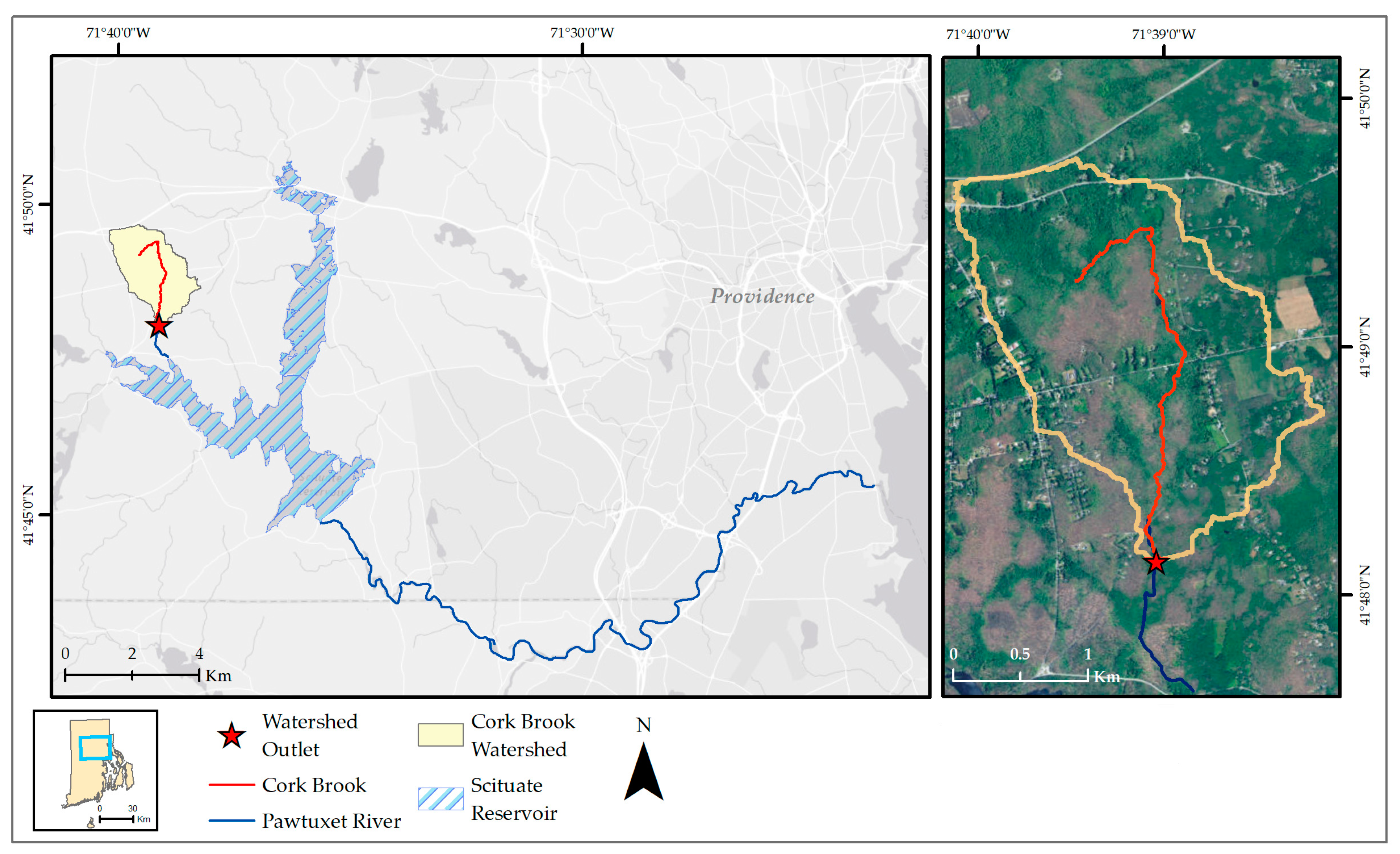
The selected study site was Cork Brook in Scituate, Rhode Island. This small forested watershed is a tributary to the Scituate Reservoir, which is part of the larger Pawtuxet River basin beginning in north-central Rhode Island and eventually flowing into Narragansett Bay. The Scituate Reservoir is the largest open body of water in the state and is the main drinking water source to the City of Providence. Human disturbance within the Cork Brook watershed is minimal, and most of the land cover is undeveloped forest and brushland; however, a portion (14%) of the land use is classified as medium density residential. USGS station number 01115280 is located approximately four km downstream from the headwaters and been continuously recording streamflow at the site since 2008 and stream temperature since 2001 [43]. The mean daily discharges at the gauge are historically lowest in September (0.025 m3/s) and highest in March (0.27 m3/s), with an annual average of approximately 0.11 m3/s. Average daily stream temperature is estimated at 7.8 °C since 2001.
This study uses the hydrologic and water quality model SWAT for simulating streamflow and stream temperature. SWAT is a well-established, physically-based, semi-distributed hydrologic model created by the United States Department of Agriculture (USDA) in 1998 [17]. The model is capable of simulating on a continuous daily, monthly and long-term time-step and incorporates the effects of climate, plant and crop growth, surface runoff, evapotranspiration, groundwater flow, nutrient loading, land use and in-stream water routing to predict hydrologic response and simulate discharge, sediment and nutrient yields from mixed land use watersheds [17,44,45,46]. As a distributed parameter model, SWAT divides a watershed into hydrologic response units (HRUs) exhibiting homogenous land, soil and slope characteristics. Surface water runoff and infiltration volumes are estimated using the modified soil conservation service (SCS) 1984 curve number method, and potential evapotranspiration is estimated using the Penman-Monteith method [47,48].
The Rhode Island Geographic Information System (RIGIS) database is the main source for the spatial data used as model inputs [49]. RIGIS is a public database managed by both the Rhode Island government and private organizations. Typical SWAT model inputs in ArcSWAT [50] include topography, soil characteristics, land cover or land use and meteorological data. Information collected for this study includes the following: 2011 Land use/land cover data derived from statewide 10-m resolution National Land Cover Data imagery [51]; soil characteristics collected from a geo-referenced digital soil map from the Natural Resource Conservation Service (NRCS) Soil Survey Geographic database (SSURGO) [52]; and topography information extracted from USGS 7.5-min digital elevation models (DEMs) with a 10-m horizontal, 7-m vertical resolution. Based on the spatial data provided, the seven-km2 Cork Brook watershed was delineated into four subbasins and 27 HRU units using land use, soil and slope thresholds of 20%, 10% and 5%. Regional meteorological data from 1979 to 2014 including long term precipitation and temperature records were recorded by a National Climate Data Center weather station near the study site; the data were downloaded from Texas A&M University’s global weather data site [53,54].
The SWAT Calibration and Uncertainty Program (SWAT-CUP), Sequential Uncertainty Fitting Version 2 (SUFI-2) [55,56], was used to conduct sensitivity analysis, calibration and model validation on stream discharge from the output hydrograph. Performance was measured using the coefficient of determination and Nash-Sutcliffe Efficiency (NSE) and percent bias (PBIAS). The coefficient of determination (R2) identifies the degree of collinearity between simulated and measured data, and NSE was used as an indicator of acceptable model performance. R2 values range from 0 to 1 with a larger R2 value indicating less error variance. NSE is a normalized statistic that determines the relative magnitude of the residual variance compared to the measured data variance [57]. NSE ranges from −∞ to 1; a value at or above 0.50 generally indicates satisfactory model performance [44,58,59,60]. This evaluation statistic is a commonly used objective function for reflecting the overall fit of a hydrograph. Percent bias is the relative percentage difference between the averaged modeled and measured data time series over (n) time steps with the objective being to minimize the value [61]. The model was validated by using calibrated parameters and performance checked using NSE, R2 and percent bias.
The most recent version of SWAT (2012) estimates stream temperature from a relationship developed by Stefan and Preud’homme [17,62] that calculates the average daily water temperature based on the average daily ambient air temperature. Ficklin et al. developed another approach using a hydroclimatological component, which calculates stream temperature based on the combined influence of air temperature and hydrological inputs, such as streamflow, throughflow, groundwater inflow and snowmelt. Once the Cork Brook model was calibrated for streamflow, the hydroclimatological component was incorporated. A separate analysis of groundwater contributions to stream discharge was conducted for Cork Brook using an automated method for estimating baseflow [63]. An estimated 60% of stream discharge at Cork Brook is contributed to baseflow as opposed to overland flow. Therefore, incorporating the hydroclimatological component into the model may provide a more accurate prediction of stream temperature.
The main Equations (1) and (2) for water temperature () created by Ficklin et al. are listed below and described in the sequential paragraph:
where is the average daily temperature, K(1/h) is a bulk coefficient of heat transfer ranging from 0 to 1, TT is the travel time of water through the subbasin (h) and ε is an air temperature coefficient. The ε coefficient is an important component because it allows the water temperature to rise above 0 °C when the air temperature is below 0 °C. If air temperature is less than 0 °C, the model will set the stream temperature to 0.1 °C. These details are further discussed in the results section of the paper. The source code for the Ficklin model was downloaded from Darren Ficklin’s research webpage at Indiana State University [64]. No additional spatial data were required for the added component and no additional streamflow calibration was necessary because discharge outputs were unchanged. Stream temperature parameters associated with the hydroclimatological model component were calibrated manually with the stream temperature data recorded at USGS Gauge 01115280. The same performance metrics (NSE and R2) were used to determine model reliability for temperature simulation.
Upon model calibration and validation, output data simulated by SWAT with the hydroclimatological component were processed to determine the occurrence of stressful conditions in Cork Brook from 1980 to 2009. As previously discussed, a stressful event for this study is defined as any day where both temperature and flow extremes occur. This study used the Q25 and Q75 flow exceedance percentiles as indicators because of their general use in the field of hydrology [65,66,67] and their ecohydrological importance to coldwater fish including brook trout [11,28,30,33,68]. The most critical period for the species is typically the lowest flows of late summer to winter, and a base flow of <25% is considered poor for maintaining quality trout habitat [11,33]. A Q75 represents the lowest 25% of all daily flow rates, and a Q25 exceedance characterizes the highest 25% of all daily flow rates. Flow-exceedance probability, or flow-duration percentile, is a well-established method and generally computed using the following equation:
where P is the probability that a given magnitude will be equaled or exceeded (percent of time), M is the ranked position (dimensionless) and n is the number of events for period of record [67]. For the stressful event analysis, the exceedance probability and average daily stream temperature for each date were identified. If the day fell into the Q25 or Q75 percentile, and if the stream temperature was greater than 21 °C, then the day was tagged as being a thermally stressful event.
3. Results and Discussion
3.1. Model Calibration & Validation
3.1.1. Stream Discharge
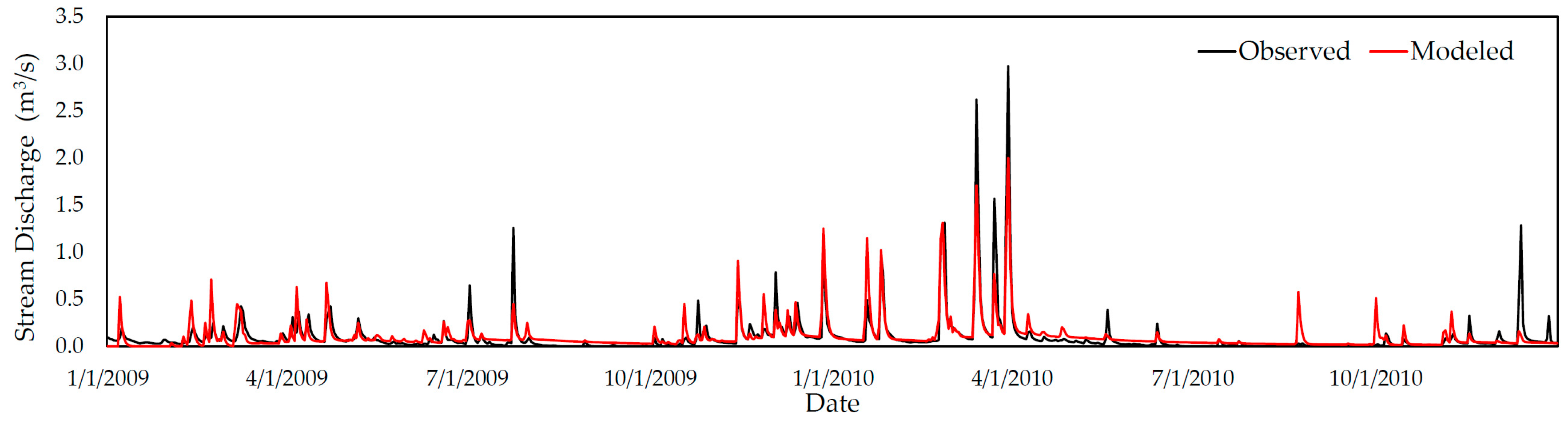
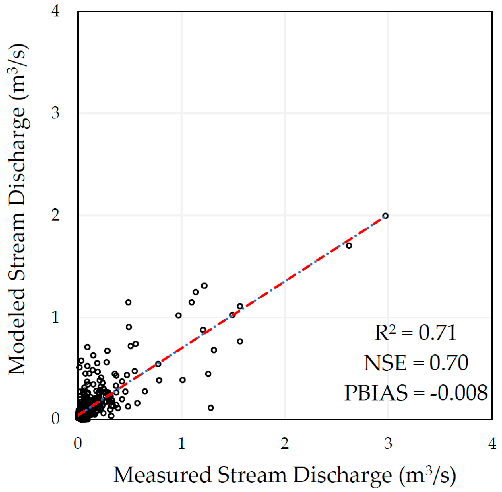
The initial model was run for the entire period of precipitation and rainfall data availability (1979–2014) and then calibrated in SWAT-CUP using a portion of the existing observed streamflow data from the USGS gauge. The model was calibrated for daily streamflow over a two-year time-span from 2009 to 2010 (Figure 2 and Figure 3) due to a limited availability in observed data (2008–present). The model was validated for the year 2012 because the 2011 data showed evidence of discharge misreading and 2013 weather data were incomplete. The hydrological parameters producing the best overall fit of the modeled hydrograph to the observed hydrograph are summarized in Table 1, and the statistical results of daily streamflow calibration and validation are shown in Table 2.
The most sensitive parameters in model calibration were primarily related to groundwater and soil characteristics. The alpha-BF (baseflow) recession value was one of the most effective parameters and had a small value of 0.049. The alpha baseflow factor is a recession coefficient derived from the properties of the aquifer contributing to baseflow; large alpha factors signify steep recession indicative of rapid drainage and minimal storage whereas low alpha values suggest a slow response to drainage [63,69]. The threshold depth of water in the shallow aquifer (GWQMN) was sensitive in model calibration and the depth of water is relatively shallow (0.6 m). This is the threshold water level in the shallow aquifer for groundwater contribution to the main channel to occur. Optimal groundwater delay was short, i.e., 1.2 days. Since groundwater accounts for the majority of stream discharge within Cork Brook, the sensitivity of soil and groundwater parameters was expected. Other factors were incorporated based on the small size of the watershed, such as surface lag time, slope length, steepness and lateral subsurface flow length, and the presence of snow at the site in the winter, such as snowmelt and snowpack temperature factors.
3.1.2. Stream Temperature
Once the initial SWAT model was satisfactorily calibrated and validated for discharge, the hydroclimatological component was added to the SWAT files and the model was run using both the basic SWAT approach and the revised stream temperature program. The hydroclimatological temperature model had no effect on stream discharge; therefore, the discharge was not re-calibrated. The hydroclimatological model was manually calibrated for stream temperature by changing several variables in the basin file associated with the hydroclimatological component: K, lag time and seasonal time periods in Julian days (Table 3). The K variable represents the relationship between air and stream temperature and ranges from 0 to 1. As K approaches 1, the stream temperature is approximately the same as air temperature, and as K decreases, the stream water is less influenced by air temperature [36]. The temperature outputs are also sensitive to the lag time, a calibration parameter corresponding to the effects of delayed surface runoff and soil water into the stream. Stream temperature was calibrated using observed data recorded by the USGS gauge from 2010 to 2011 and validated from 2012 to 2013.
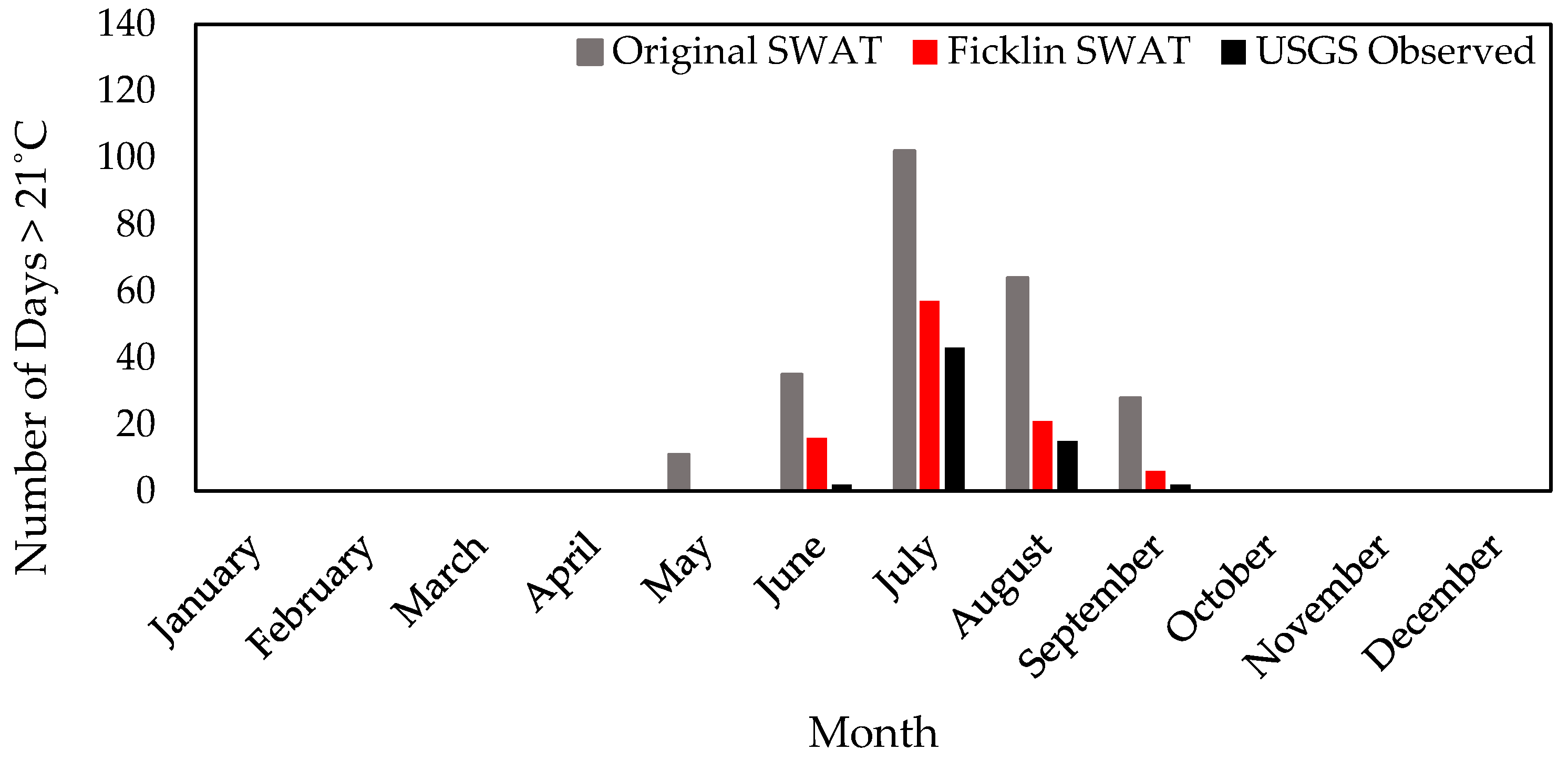
The above parameters produced satisfactory stream temperature calibration statistics for the hydroclimatological model, as summarized in Table 4. During the winter and spring, the stream temperature is roughly the same as the air. In the summer and fall, the K value is decreased and the stream temperature is less affected by air temperature. This may be due to extensive tree shading [36], which is in agreement for Cork Brook as it is a relatively small watershed that is predominantly forested [70]. The lag time is relatively short throughout the year and is similar to the surface and groundwater delay parameters set during stream discharge calibration. The Ficklin et al. approach generated comparable R2 value but a higher NSE than the basic SWAT approach. More importantly, the hydroclimatological model better predicted the occurrence of stressful stream temperatures compared to the original SWAT model during the calibration and validation periods (Figure 4). Therefore, since stream temperature is the main driving component in which a situation is considered stressful for brook trout, the hydroclimatological model appears less likely to over-predict stressful conditions than the original SWAT model.
3.2. Stream Conditions and Stressful Event Analysis
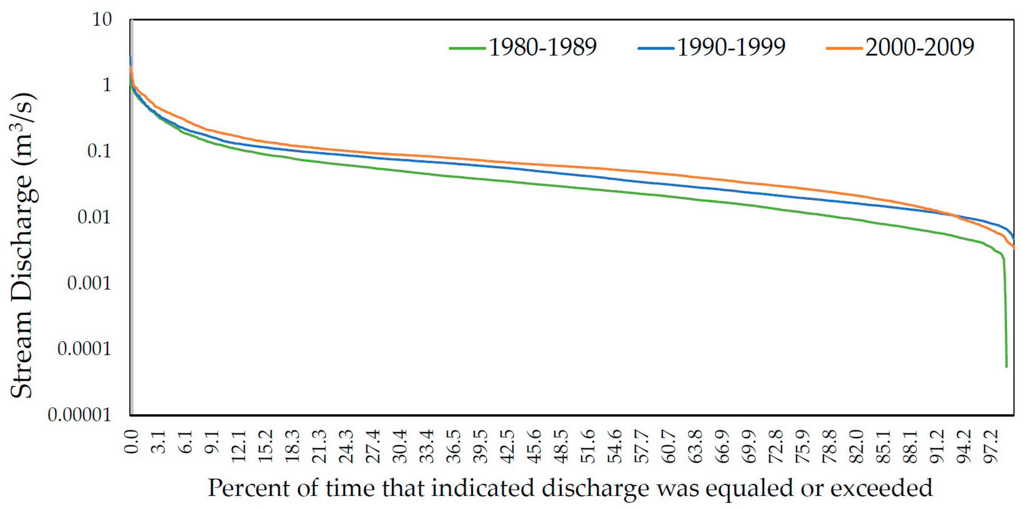
The SWAT model incorporating the added hydroclimatological component was used for stressful event analysis, as it proved to be more accurate than the basic SWAT model. The model predicted an increase in the magnitude of stream discharge increases by each decade between 1980 and 2009, as shown in Figure 5, although the shape of the flow duration curve stayed relatively consistent. The simulated stream discharge rates increased as well, averaging 0.06 m3/s in 1980–1989, 0.08 m3/s in 1990–1999 and 0.10 m3/s between 2000 and 2009. The maximum streamflow fluctuated, 1.74 m3/s in 1980–1989, 2.75 m3/s in 1990–1999 and 1.93 m3/s between 2000 and 2009. Several existing studies have examined how the climate has changed over the last 30-years in New England. Since 1970, Rhode Island’s annual precipitation has increased 6–11%. Fewer days with snow cover and earlier ice-out dates are occurring [71,72]. A large-scale regional study [1] collected climate and streamflow data from 27 USGS stream gauges recorded for a historical average of 71 years throughout the New England region. The study indicated that there were increases over time in annual maximum streamflows. The stream discharge results produced by the Cork Brook model align well with what has been observed statewide and across New England and support claims that certain effects of climate change are already beginning to take place.
As water temperatures increase due to global warming, brook trout may benefit from sustained flows which will prevent stream temperatures from rising further and help ensure that downstream habitat remains connected to headwaters. On the other hand, a sustained increase in flow magnitude can change the geomorphology and may not be beneficial for aquatic species during the spawning season when flows are normally lower [30]. An increase in stream discharges during the low flow season may put redds at risk of destruction from sedimentation or sheer velocity. Changes in streamflow magnitude may also increase turbidity or redistribute riffle and pool habitat throughout the stream reach. This may decrease the availability of suitable habitat as brook trout prefer stream reaches with an approximate 1:1 pool-riffle ratio [11]. Pool and riffle redistribution can also affect the type and quantity of local macroinvertebrate populations. Since warming temperatures will have an impact on body condition as fish enter the winter months, the available food supply can become an even more critical factor as the climate changes.
To identify the number of stressful events simulated by the model, output data were analyzed by decade (1980–1989, 1990–1999 and 2000–2009) and over the entire 30-year period. The percent chance that a stressful event would occur on any given day throughout the time period was also calculated. These results are shown in Table 5 below.
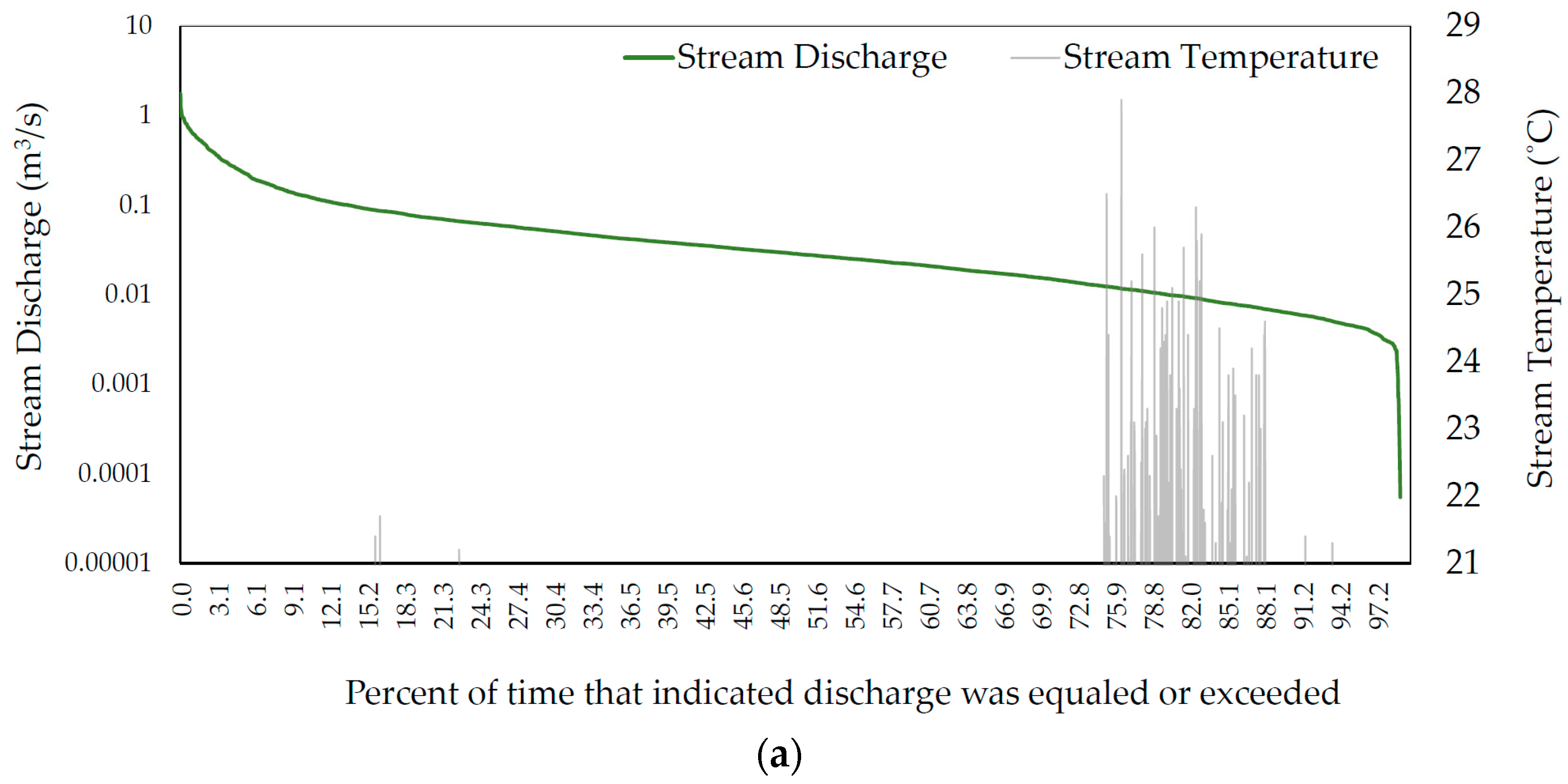
The model predicted an increase in the number of stressful events between 1980 and 2009 with the greatest change taking place between the first decade (1980–1989) and the second decade (1990–2009). It is interesting to note that although the model predicted an increase in number of stressful events between 1980 and 2009, the number of temperature stress days and the number of flow stress days generally decreased between decades (Table 5). Figure 6 have been created to gain a better understanding of how the co-occurrence of temperature stress and the flow stress has changed in Cork Brook.
The graphs show that of all 338 stressful events simulated between 1980 and 2009, only seven events occurred within the Q25 flow percentiles. The remaining events simulated by the model occurred when flows were within the Q75–Q97 flow percentile because lower, slower flows are exposed to air longer, causing them to increase or decrease in temperature more easily. The fact that there were no stressful events above the Q97 flow percentiles is most likely attributed to groundwater inputs. During the dry or low flow periods in summer and fall, baseflow will be the primary input to groundwater fed streams. Because the hydroclimatological model component takes the groundwater temperature into consideration, the lowest discharge amounts the model simulates will likely be baseflow driven and therefore cooler than water that is continuously exposed to ambient air temperatures. This is good news for coldwater fish species which spawn in the fall or those that begin their migration into headwaters during the low flow season, as the chance of exposure to high temperatures is lessened from groundwater contributions.
The greatest change in the number of stressful events occurred between the first and second decades where the count of stressful events increased from 84 in 1980–1989 to 122 in 1990–1999. Comparing Figure 6, the stressful events stretch from Q75 to Q87 in 1980–1989, whereas in 1990–1999 the events extend into the Q96 percentile. This shows that a combination of flow and temperature should be taken into consideration when making management decisions or evaluating the quality of aquatic habitat. For instance, managers can be reassured that withdrawing water during Q25 flows will not be as harmful to fish as withdrawing during Q75 flows. During drought years, it may become tempting to withdraw additional groundwater resources. However, the knowledge that groundwater can help reduce the occurrence of stressful events to fish during low flows may influence a manager’s choice. Because Cork Brook is upstream from the Scituate Reservoir, water resource management decisions are especially applicable to this watershed.
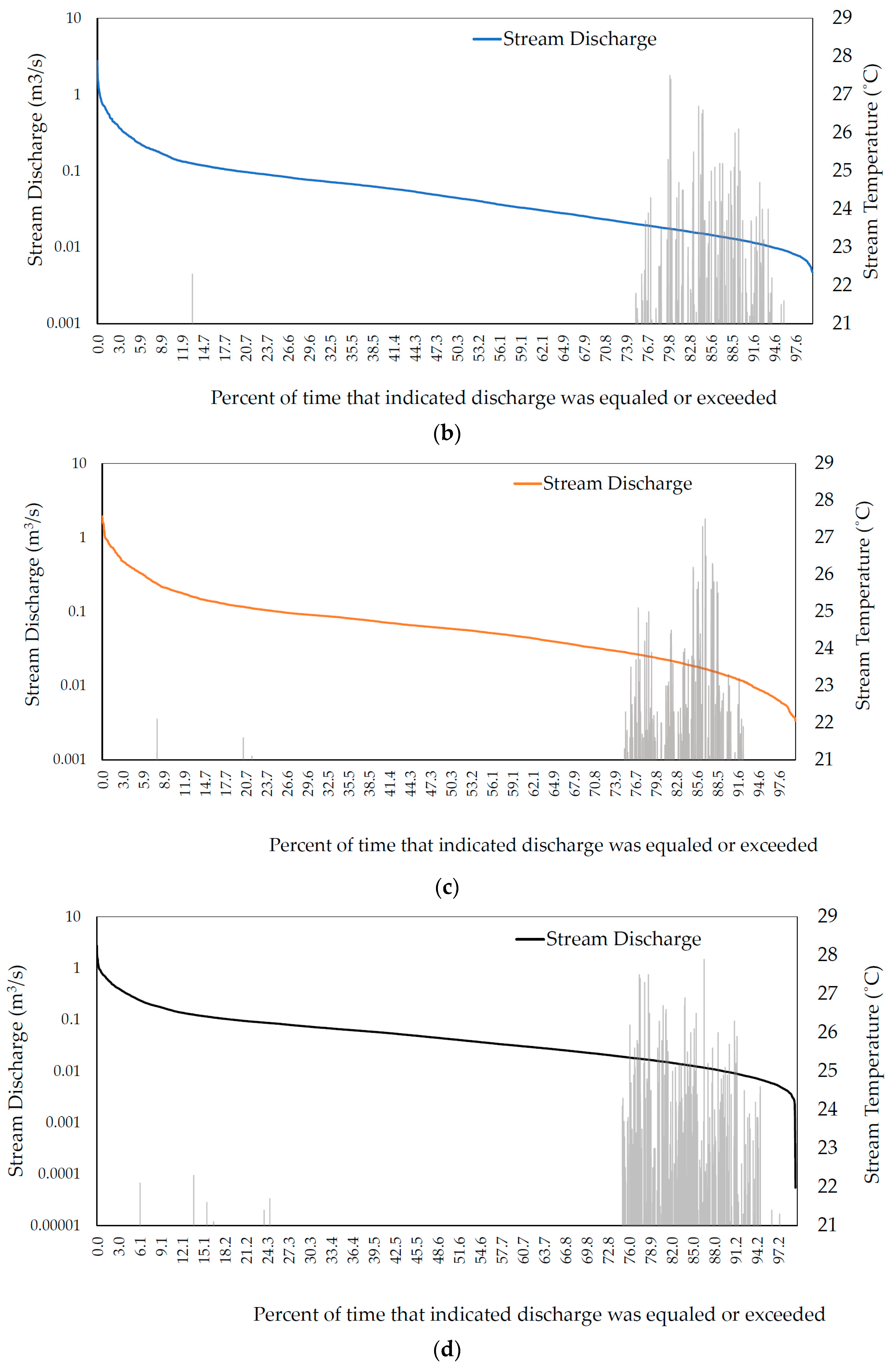
Further analysis of 2-, 7- and 10-day moving averages at the lowest 25th percentile flow suggested that the majority of high stream temperatures are occurring during the 2-day low flow conditions as opposed to the 7-day and 10-day low flows (Figure 7). Such details can have important implications for aquatic species. Brook trout have been observed to tolerate higher stream temperatures provided their physical habitat remains stable [34]. If the co-occurrence of temperature and flow stresses last longer, then physiological stresses to individual trout may become more apparent. The data simulated from 1980 to 2009 provide a helpful baseline for comparing future projections and will help determine if the resilience of local brook trout populations may become strained under future climate conditions.
4. Conclusions and Future Work
Since the hydroclimatological model was shown to be more accurate, future research projects should consider using the new component in similar watersheds throughout the region for both historical and climate change assessments. This study found that the long-term historical stream temperature data recorded by the USGS gauge at Cork Brook were necessary for model calibration. Therefore, scientists should have a reliable set of observed stream temperature data to calibrate and validate the stream temperature output, especially if studying ecosystems that are particularly sensitive to temperature related parameters. Other related future work may include applying the methodology to other types of temperature-sensitive aquatic organisms such as certain macroinvertebrate species. Macroinvertebrates form part of the base of the food chain, and fluctuations in their population or distributions throughout a stream reach can impact higher trophic level species that prey on these organisms.
Another consideration for future work is to limit the stressful event analysis to the spring and summer months when brook trout are more sensitive to warmer stream temperatures. Also, a study could be conducted to see if stressful events occur sequentially. This study took a wider approach by examining how stream temperatures and streamflow vary throughout the entire year. This timeframe was chosen for several reasons. First, since this is the only study of its kind within these watersheds, we did not have enough information to say with certainty that no changes to stream temperature or streamflow would occur during the fall and winter. In fact, some scientists predict that by the end of the century Rhode Island will have a climate similar to that of Georgia [71], in which case stream temperatures would almost certainly increase during the winter months. Second, while stream temperatures and streamflow during the winter months are not as critical for brook trout compared to the summer, winter conditions do effect embryo development. For instance, the length of embryo incubation during the winter ranges from 28 to 45 days depending on the temperature of the stream water [11]. Lastly, while this study focused on brook trout, our hope is that the methodology can be applied to other types of aquatic species that may be sensitive to stream conditions during other seasons.
The purpose of this study was to gain a better understanding of the historical conditions in coldwater habitat using SWAT. We successfully showed that SWAT with the hydroclimatological component is more accurate than the original SWAT model at this forested, baseflow driven watershed in Rhode Island. Moreover, thermally stressful event identification is a functional approach to analyzing model output. The data simulated from 1980 to 2009 provide a helpful baseline for comparing future projections by combining two important indicators for the survival of coldwater species.
Acknowledgments
We would like to acknowledge Thomas Boving of the University of Rhode Island and Jameson Chace of Salve Regina University for their insight and review of this Master’s thesis project. This research project is supported by S-1063 Multistate Hatch Project.
Author Contributions
B.C. and S.M.P. conceived and designed the experiments; B.C. performed the experiments; B.C., S.M.P. and A.J.G. analyzed the data; B.C. wrote the paper.
Conflicts of Interest
The authors declare no conflict of interest.
References
- Hodgkins, G.A.; Dudley, R.W.; Huntington, T.G. Changes in the timing of high river flows in New England over the 20th century. J. Hydrol. 2003, 278, 244–252. [Google Scholar] [CrossRef]
- Hayhoe, K.; Wake, C.P.; Huntington, T.G.; Luo, L.; Schwartz, M.D.; Sheffield, J.; Wood, E.; Anderson, B.; Bradbury, J.; DeGaetano, A.; et al. Past and future changes in climate and hydrological indicators in the US Northeast. Clim. Dyn. 2007, 28, 381–407. [Google Scholar] [CrossRef]
- Eaton, J.G.; Scheller, R.M. Effects of climate warming on fish thermal habitat in streams of the United States. Limnol. Oceanogr. 1996, 41, 1109–1115. [Google Scholar] [CrossRef]
- Mohseni, O.; Stefan, H.G.; Eaton, J.G. Global warming and potential changes in fish habitat in U.S. Streams. Clim. Chang. 2003, 59, 389–409. [Google Scholar] [CrossRef]
- Woodward, G.; Perkins, D.M.; Brown, L.E. Climate change and freshwater ecosystems: Impacts across multiple levels of organization. Philos. Trans. R. Soc. B Biol. Sci. 2010, 365, 2093–2106. [Google Scholar] [CrossRef] [PubMed]
- Jiménez Cisneros, B.E.; Oki, T.; Arnell, N.W.; Benito, G.; Cogley, J.G.; Doll, P.; Jiang, T.; Mwakalila, S.S. 2014: Freshwater Resources. In Climate Change 2014: Impacts, Adaptation and Vulnerability. Part A: Global and Sectoral Aspects; Contribution of Working Group II to the Fifth Assessment Report of the Intergovernmental Panel on Climate Change; Cambridge University Press: Cambridge, UK; New York, NY, USA, 2014; p. 40. [Google Scholar]
- Whitney, J.E.; Al-Chokhachy, R.; Bunnell, D.B.; Caldwell, C.A.; Cooke, S.J.; Eliason, E.J.; Rogers, M.; Lynch, A.J.; Paukert, C.P. Physiological basis of climate change impacts on North American inland fishes. Fisheries 2016, 41, 332–345. [Google Scholar] [CrossRef]
- Mohseni, O.; Erickson, T.R.; Stefan, H.G. Sensitivity of stream temperatures in the United States to air temperatures projected under a global warming scenario. Water Resour. Res. 1999, 35, 3723–3733. [Google Scholar] [CrossRef]
- Van Vliet, M.T.H.; Franssen, W.H.P.; Yearsley, J.R.; Ludwig, F.; Haddeland, I.; Lettenmaier, D.P.; Kabat, P. Global river discharge and water temperature under climate change. Glob. Environ. Chang. 2013, 23, 450–464. [Google Scholar] [CrossRef]
- Brett, J.R. Some principles in the thermal requirements of fishes. Q. Rev. Biol. 1956, 31, 75–87. [Google Scholar] [CrossRef]
- Raleigh, R.F. Habitat Suitability Index Models: Brook Trout; 82/10.24; U.S. Fish and Wildlife Service: Washington, DC, USA, 1982.
- Fry, F.E.J. The effect of environmental factors on the physiology of fish. In Fish Physiology; Hoar, W.S., Randall, D.J., Eds.; Academic Press: Cambridge, MA, USA, 1971; Volume 6, pp. 1–98. [Google Scholar]
- Hokanson, K.E.F.; McCormick, J.H.; Jones, B.R.; Tucker, J.H. Thermal requirements for maturation, spawning, and embryo survival of the brook trout, Salvelinus fontinalis. J. Fish. Res. Board Can. 1973, 30, 975–984. [Google Scholar] [CrossRef]
- Milner, N.J.; Elliott, J.M.; Armstrong, J.D.; Gardiner, R.; Welton, J.S.; Ladle, M. The natural control of salmon and trout populations in streams. Fish. Res. 2003, 62, 111–125. [Google Scholar] [CrossRef]
- Goniea, T.M.; Keefer, M.L.; Bjornn, T.C.; Peery, C.A.; Bennett, D.H.; Stuehrenberg, L.C. Behavioral thermoregulation and slowed migration by adult fall chinook salmon in response to high Columbia River water temperatures. Trans. Am. Fish. Soc. 2006, 135, 408–419. [Google Scholar] [CrossRef]
- Peterson, J.T.; Kwak, T.J. Modeling the effects of land use and climate change on riverine smallmouth bass. Ecol. Appl. 1999, 9, 1391–1404. [Google Scholar] [CrossRef]
- Arnold, J.G.; Srinivasan, R.; Muttiah, R.S.; Williams, J.R. Large area hydrologic modeling and assessment part I: Model development. JAWRA J. Am. Water Resour. Assoc. 1998, 34, 73–89. [Google Scholar] [CrossRef]
- Erkan, D.E. Strategic Plan for the Restoration of Anadromous Fishes to Rhode Island Coastal Streams; Rhode Island Department of Environmental Management, Division of Fish and Wildlife: Providence, RI, USA, 2002.
- WPWA. Maximum Daily Stream Temperature in the Queen River Watershed and Mastuxet Brook Summer 2006. Wood-Pawcatuck Watershed Association. Available online: http://www.wpwa.org/reports/2006TemperatureStudy.pdf (accessed on 1 October 2016).
- Hakala, J.P.; Hartman, K.J. Drought effect on stream morphology and brook trout (Salvelinus fontinalis) populations in forested headwater streams. Hydrobiologia 2004, 515, 203–213. [Google Scholar] [CrossRef]
- Chadwick, J.J.G.; Nislow, K.H.; McCormick, S.D. Thermal onset of cellular and endocrine stress responses correspond to ecological limits in brook trout, an iconic cold-water fish. Conserv. Physiol. 2015, 3, cov017. [Google Scholar] [CrossRef] [PubMed]
- Letcher, B.H.; Nislow, K.H.; Coombs, J.A.; O’Donnell, M.J.; Dubreuil, T.L. Population response to habitat fragmentation in a stream-dwelling brook trout population. PLoS ONE 2007, 2, e1139. [Google Scholar] [CrossRef] [PubMed]
- Lee, R.M.; Rinne, J.N. Critical thermal maxima of five trout species in the southwestern United States. Trans. Am. Fish. Soc. 1980, 109, 632–635. [Google Scholar] [CrossRef]
- Bjornn, T.; Reiser, D. Habitat requirements of salmonids in streams. Am. Fish. Soc. Spec. Publ. 1991, 19, 138. [Google Scholar]
- Kling, G.W.; Hayhoe, K.; Johnson, L.B.; Magnuson, J.J.; Polasky, S.; Robinson, S.K.; Shuter, B.J.; Wander, M.M.; Wuebbles, D.J.; Zak, D.R. Confronting Climate Change in the Great Lakes Region: Impacts on Our Communities and Ecosystems; Union of Concerned Scientists: Cambridge, MA, USA; Ecological Society of America: Washington, DC, USA, 2003; p. 92. [Google Scholar]
- Magnuson, J.J.; Crowder, L.B.; Medvick, P.A. Temperature as an ecological resource. Am. Zool. 1979, 19, 331–343. [Google Scholar] [CrossRef]
- Vannote, R.L.; Minshall, G.W.; Cummins, K.W.; Sedell, J.R.; Cushing, C.E. The river continuum concept. Can. J. Fish. Aquat. Sci. 1980, 37, 130–137. [Google Scholar] [CrossRef]
- Bunn, S.E.; Arthington, A.H. Basic principles and ecological consequences of altered flow regimes for aquatic biodiversity. Environ. Manag. 2002, 30, 492–507. [Google Scholar] [CrossRef]
- Freeman, M.C.; Pringle, C.M.; Jackson, C.R. Hydrologic connectivity and the contribution of stream headwaters to ecological integrity at regional scales. JAWRA J. Am. Water Resour. Assoc. 2007, 43, 5–14. [Google Scholar] [CrossRef]
- Poff, N.L.; Allan, J.D. Functional organization of stream fish assemblages in relation to hydrological variability. Ecology 1995, 76, 606–627. [Google Scholar] [CrossRef]
- Poff, N.L.; Allan, J.D.; Bain, M.B.; Karr, J.R.; Prestegaard, K.L.; Richter, B.D.; Sparks, R.E.; Stromberg, J.C. The natural flow regime. BioScience 1997, 47, 769–784. [Google Scholar] [CrossRef]
- Bassar, R.D.; Letcher, B.H.; Nislow, K.H.; Whiteley, A.R. Changes in seasonal climate outpace compensatory density-dependence in eastern brook trout. Glob. Chang. Biol. 2016, 22, 577–593. [Google Scholar] [CrossRef] [PubMed]
- DePhilip, M.; Moberg, T. Ecosystem Flow Recommendations for the Susquehanna River Basin; The Nature Conservancy: Harrisburg, PA, USA, 2010. [Google Scholar]
- Nuhfer, A.J.; Zorn, T.G.; Wills, T.C. Effects of reduced summer flows on the brook trout population and temperatures of a groundwater-influenced stream. Ecol. Freshw. Fish 2017, 26, 108–119. [Google Scholar] [CrossRef]
- Walters, A.W.; Post, D.M. An experimental disturbance alters fish size structure but not food chain length in streams. Ecology 2008, 89, 3261–3267. [Google Scholar] [CrossRef] [PubMed]
- Ficklin, D.L.; Luo, Y.; Stewart, I.T.; Maurer, E.P. Development and application of a hydroclimatological stream temperature model within the soil and water assessment tool. Water Resour. Res. 2012, 48. [Google Scholar] [CrossRef]
- Hayhoe, K.; Wake, C.; Anderson, B.; Liang, X.-Z.; Maurer, E.; Zhu, J.; Bradbury, J.; DeGaetano, A.; Stoner, A.M.; Wuebbles, D. Regional climate change projections for the northeast USA. Mitig. Adapt. Strateg. Glob. Chang. 2008, 13, 425–436. [Google Scholar] [CrossRef]
- Isaak, D.J.; Wollrab, S.; Horan, D.; Chandler, G. Climate change effects on stream and river temperatures across the northwest U.S. from 1980–2009 and implications for salmonid fishes. Clim. Chang. 2012, 113, 499–524. [Google Scholar] [CrossRef]
- Mohseni, O.; Stefan, H.G. Stream temperature/air temperature relationship: A physical interpretation. J. Hydrol. 1999, 218, 128–141. [Google Scholar] [CrossRef]
- Null, S.; Viers, J.; Deas, M.; Tanaka, S.; Mount, J. Stream temperature sensitivity to climate warming in California’s Sierra Nevada. In Proceedings of the AGU Fall Meeting Abstracts, San Francisco, CA, USA, 13–17 December 2010. [Google Scholar]
- Preud’homme, E.B.; Stefan, H.G. Relationship between Water Temperatures and Air Temperatures for Central US Streams; EPA/600/R-92/243; U.S. Environmental Protection Agency: Washington, DC, USA, 2002.
- Brennan, L. Stream Temperature Modeling: A Modeling Comparison for Resource Managers and Climate Change Analysis. Master’s Thesis, University of Massachusetts, Amherst, MA, USA, 2015. [Google Scholar]
- US Geological Survey (USGS). U.G.S. National Water Information System Web Interface, 2015 ed.; US Geological Survey: Reston, VA, USA, 2017.
- Douglas-Mankin, K.R.; Srinivasan, R.; Arnold, J.G. Soil and water assessment tool (SWAT) model: Current developments and applications. Trans. ASABE 2010, 53, 1423–1431. [Google Scholar] [CrossRef]
- Gassman, P.W.; Reyes, M.R.; Green, C.H.; Arnold, J.G. The soil and water assessment tool: Historical development, applications, and future research directions. Trans. ASABE 2007, 50, 1211–1250. [Google Scholar] [CrossRef]
- Neitsch, S.L.; Arnold, J.G.; Kiniry, J.R.; Williams, J.R. Soil and Water Assessment Tool Theoretical Documentation Version 2009; Texas Water Resources Institute: College Station, TX, USA, 2011. [Google Scholar]
- Penman, H.L. Estimating evaporation. Eos Trans. Am. Geophys. Union 1956, 37, 43–50. [Google Scholar] [CrossRef]
- Monteith, J.L. Evaporation and environment. Symp. Soc. Exp. Biol. 1965, 19, 205–234. [Google Scholar] [PubMed]
- University of Rhode Island. Rhode Island Geographic Information System (RIGIS); University of Rhode Island Rhode Island: Kingston, RI, USA, 2016; Available online: http://www.rigis.org (accessed on 3 September 2017).
- Texas A&M University. Arcswat Software; ArcSWAT 2012.10.19; Texas A&M University: College Station, TX, USA, 2012; Available online: http://swat.tamu.edu/ (accessed on 3 September 2017).
- Homer, C.G.; Dewitz, J.A.; Yang, L.; Jin, S.; Danielson, P.; Xian, G.; Coulston, J.; Herold, N.D.; Wickham, J.; Megown, K. Completion of the 2011 national land cover database for the conterminous United States—Representing a decade of land cover change information. Photogramm. Eng. Remote Sens. 2015, 81, 345–354. [Google Scholar]
- Rhode Island Geographic Information System (RIGIS). Data Distribution System SOIL_soils. Available online: http://www.rigis.org/geodata/soil/Soils16.zip (accessed on 5 September 2016).
- Saha, S.; Moorthi, S.; Wu, X.; Wang, J.; Nadiga, S.; Tripp, P.; Behringer, D.; Hou, Y.-T.; Chuang, H.-Y.; Iredell, M.; et al. The ncep climate forecast system version 2. J. Clim. 2014, 27, 2185–2208. [Google Scholar] [CrossRef]
- Texas A&M University. NCEP Global Weather Data for Swat. Available online: http://swat.tamu.edu/ (accessed on 3 January 2016).
- Abbaspour, K.C. SWAT Calibration and Uncertainty Program—A User Manual; Swat-Cup 2012; Swiss Federal Institute of Aquatic Science and Technology, Eawag: Duebendorf, Switzerland, 2013. [Google Scholar]
- Abbaspour, K. User Manual for Swat-Cup, Swat Calibration and Uncertainty Analysis Programs; Swiss Federal Institute of Aquatic Science and Technology, Eawag: Duebendorf, Switzerland, 2007. [Google Scholar]
- Nash, J.E.; Sutcliffe, J.V. River flow forecasting through conceptual models part I—A discussion of principles. J. Hydrol. 1970, 10, 282–290. [Google Scholar] [CrossRef]
- Moriasi, D.N.; Arnold, J.G.; Liew, M.W.V.; Bingner, R.L.; Harmel, R.D.; Veith, T.L. Model evaluation guidelines for systematic quantification of accuracy in watershed simulations. Trans. ASABE 2007, 50, 885–900. [Google Scholar] [CrossRef]
- Singh, J.; Knapp, H.V.; Arnold, J.G.; Demissie, M. Hydrological modeling of the iroquois river watershed using HSPF and SWAT. JAWRA J. Am. Water Resour. Assoc. 2005, 41, 343–360. [Google Scholar] [CrossRef]
- Liew, M.W.V.; Veith, T.L.; Bosch, D.D.; Arnold, J.G. Suitability of swat for the conservation effects assessment project: Comparison on usda agricultural research service watersheds. J. Hydrol. Eng. 2007, 12, 173–189. [Google Scholar] [CrossRef]
- Pradhanang, S.M.; Mukundan, R.; Schneiderman, E.M.; Zion, M.S.; Anandhi, A.; Pierson, D.C.; Frei, A.; Easton, Z.M.; Fuka, D.; Steenhuis, T.S. Streamflow responses to climate change: Analysis of hydrologic indicators in a New York city water supply watershed. JAWRA J. Am. Water Resour. Assoc. 2013, 49, 1308–1326. [Google Scholar] [CrossRef]
- Stefan, H.G.; Preud’homme, E.B. Stream temperature estimation from air temperature. JAWRA J. Am. Water Resour. Assoc. 1993, 29, 27–45. [Google Scholar] [CrossRef]
- Arnold, J.G.; Allen, P.M.; Muttiah, R.; Bernhardt, G. Automated base flow separation and recession analysis techniques. Ground Water 1995, 33, 1010–1018. [Google Scholar] [CrossRef]
- Ficklin, D.L. Swat Stream Temperature Executable Code; Indiana State University: Terre Haute, IN, USA, 2012. [Google Scholar]
- Pyrce, R. Hydrological Low Flow Indices and Their Uses; Watershed Science Centre (WSC) Report; Trent University: Peterborough, ON, Canada, 2004. [Google Scholar]
- Smakhtin, V.U. Low flow hydrology: A review. J. Hydrol. 2001, 240, 147–186. [Google Scholar] [CrossRef]
- Ahearn, E.A. Flow Durations, Low-Flow Frequencies, and Monthly Median Flows for Selected Streams in Connecticut through 2005; US Department of the Interior: Washington, DC, USA; US Geological Survey: Reston, VA, USA, 2008.
- Armstrong, D.S.; Richards, T.A.; Parker, G.W. Assessment of Habitat, Fish Communities, and Streamflow Requirements for Habitat Protection, Ipswich River, Massachusetts, 1998–99; Department of the Interior, US Geological Survey: Reston, VA, USA, 2001.
- Arnold, J.G.; Allen, P.M. Automated methods for estimating baseflow and ground water recharge from streamflow records. JAWRA J. Am. Water Resour. Assoc. 1999, 35, 411–424. [Google Scholar] [CrossRef]
- Johnson, S.L. Factors influencing stream temperatures in small streams: Substrate effects and a shading experiment. Can. J. Fish. Aquat. Sci. 2004, 61, 913–923. [Google Scholar] [CrossRef]
- Wake, C.P.; Keeley, C.; Burakowski, E.; Wilkinson, P.; Hayhoe, K.; Stoner, A.; LaBrance, J. Climate Change in Northern New Hampshire: Past, Present and Future; Climate Solutions New England: Durham, NH, USA, 2014. [Google Scholar]
- Wake, C. Rhode Island’s Climate: Past and Future Changes; Climate Solutions New England: Durham, NH, USA, 2014; p. 2. [Google Scholar]
Figure 1.
The Cork Brook watershed empties into the Scituate Reservoir, the main drinking water supply for the City of Providence, Rhode Island, USA.
Figure 1.
The Cork Brook watershed empties into the Scituate Reservoir, the main drinking water supply for the City of Providence, Rhode Island, USA.

Figure 2.
A simulated 2009–2010 hydrograph produced by the calibrated Cork Brook SWAT model compared to observed data from USGS Gauge 01115280.
Figure 2.
A simulated 2009–2010 hydrograph produced by the calibrated Cork Brook SWAT model compared to observed data from USGS Gauge 01115280.

Figure 3.
Streamflow scatterplot of modeled and observed average daily streamflow from USGS gauge 0111528 during 2009–2010.
Figure 3.
Streamflow scatterplot of modeled and observed average daily streamflow from USGS gauge 0111528 during 2009–2010.

Figure 4.
The number of days per month that stream temperatures exceeded the stress threshold of 21 °C during the stream temperature calibration and validation periods (2010–2013).
Figure 4.
The number of days per month that stream temperatures exceeded the stress threshold of 21 °C during the stream temperature calibration and validation periods (2010–2013).

Figure 5.
Simulated flow duration curves by decade generated by the SWAT model with the hydroclimatological component. Stream discharge is equal to zero at the 100th percentile.
Figure 5.
Simulated flow duration curves by decade generated by the SWAT model with the hydroclimatological component. Stream discharge is equal to zero at the 100th percentile.

Figure 6.
Cork Brook simulated flow duration curve and stream temperatures for SWAT with the hydroclimatological component over three decades. (a) 1980–1989, (b) 1990–1999 (c) 2000–2009 and (d) 1980–2009. The secondary y-axis begins at 21 °C and any temperatures that are not above the stressful threshold are not shown in the figures. The stream temperatures in the Q25–Q75 range are omitted from each figure.


Figure 7.
The number of days per decade that stream temperatures exceeded the stress threshold of 21 °C during the 2-, 7- and 10-day moving averages at the lowest 25th flow percentile.
Figure 7.
The number of days per decade that stream temperatures exceeded the stress threshold of 21 °C during the 2-, 7- and 10-day moving averages at the lowest 25th flow percentile.


Table 1.
Range of values for the most sensitive parameters in SWAT streamflow calibration using SWAT-CUP. The parameter is listed by name and SWAT input file type, definition and the range of values that were selected for the model.
Table 1.
Range of values for the most sensitive parameters in SWAT streamflow calibration using SWAT-CUP. The parameter is listed by name and SWAT input file type, definition and the range of values that were selected for the model.
| Parameter | Definition | Value Range | Units |
|---|---|---|---|
| CN2.mgt | SCS runoff curve number | −0.40–0.75 | - |
| ALPHA_BF.gw | Baseflow alpha factor | 0.0–0.10 | 1/Days |
| GW_DELAY.gw | Groundwater delay | 0.0–7.0 | Days |
| GWQMN.gw | Depth of water in shallow aquifer for return flow | 200–1000 | mm |
| v__SMTMP.bsn | Snowmelt base temperature | −0.5–2.0 | °C |
| ESCO.hru | Soil evaporation compensation factor | 0.15–0.65 | - |
| EPCO.hru | Plant uptake compensation factor | 0.15–65 | - |
| SLSOIL.hru | Slope length for lateral subsurface flow | 0.0–150.0 | m |
Table 2.
Statistical results produced by SWAT-CUP for daily stream discharge using the parameters listed in Table 1.
Table 2.
Statistical results produced by SWAT-CUP for daily stream discharge using the parameters listed in Table 1.
| Streamflow | R2 | NSE | PBIAS |
|---|---|---|---|
| Calibration | 0.70 | 0.71 | −0.01 |
| Validation | 0.54 | 0.50 | 0.03 |
Table 3.
Hydroclimatological SWAT calibration parameters for daily stream temperature. Time period is in Julian days and the lag unit is days.
Table 3.
Hydroclimatological SWAT calibration parameters for daily stream temperature. Time period is in Julian days and the lag unit is days.
| Time Period | Alpha | Beta | Phi | K | Lag Time |
|---|---|---|---|---|---|
| 1–180 | 1.0 | 1.0 | 1.0 | 1.0 | 4 |
| 181–270 | 1.0 | 1.0 | 0.8 | 0.8 | 2 |
| 271–330 | 1.0 | 1.0 | 0.8 | 0.8 | 2 |
| 331–366 | 1.0 | 1.0 | 1.0 | 0.7 | 4 |
Table 4.
Statistical results of the daily stream temperature calibration. The average recorded stream temperature at the USGS gauge is 7.8 °C.
Table 4.
Statistical results of the daily stream temperature calibration. The average recorded stream temperature at the USGS gauge is 7.8 °C.
| Model Type | R2 | NSE | Mean Stream Temperature |
|---|---|---|---|
| Basic SWAT Calibration | 0.93 | 0.83 | 12.5 °C |
| Basic SWAT Validation | 0.94 | 0.83 | 12.9 °C |
| Ficklin Calibration | 0.95 | 0.93 | 9.9 °C |
| Ficklin Validation | 0.96 | 0.94 | 10.0 °C |
Table 5.
Stressful event analysis of SWAT with the hydroclimatological component. Shown is the percent chance that of the 3653 days per each decade and 10,958 days between 1980 and 2009, a day with any type of stress will occur, a day with flow stress will occur, a day with temperature stress will occur and the percent chance of an event.
| Date | Indicator | Any Type of Stress | Stream Temp. >21 °C | Q25 or Q75 Flow | Stressful Event |
|---|---|---|---|---|---|
| 1980–1989 | Days | 2066 | 252 | 1814 | 84 |
| % Chance | 56.6 | 6.9 | 49.7 | 2.3 | |
| 1990–1999 | Days | 2049 | 228 | 1821 | 122 |
| % Chance | 56.1 | 6.2 | 49.8 | 3.3 | |
| 2000–2009 | Days | 2007 | 196 | 1811 | 131 |
| % Chance | 54.9 | 5.4 | 49.6 | 3.6 | |
| 1980–2009 | Days | 6142 | 676 | 5466 | 338 |
| % Chance | 56.0 | 6.2 | 49.9 | 3.1 |
© 2017 by the authors. Licensee MDPI, Basel, Switzerland. This article is an open access article distributed under the terms and conditions of the Creative Commons Attribution (CC BY) license (http://creativecommons.org/licenses/by/4.0/).
Share and Cite
MDPI and ACS Style
Chambers, B.; Pradhanang, S.M.; Gold, A.J. Assessing Thermally Stressful Events in a Rhode Island Coldwater Fish Habitat Using the SWAT Model. Water 2017, 9, 667. https://0-doi-org.brum.beds.ac.uk/10.3390/w9090667
AMA Style
Chambers B, Pradhanang SM, Gold AJ. Assessing Thermally Stressful Events in a Rhode Island Coldwater Fish Habitat Using the SWAT Model. Water. 2017; 9(9):667. https://0-doi-org.brum.beds.ac.uk/10.3390/w9090667
Chicago/Turabian StyleChambers, Britta, Soni M. Pradhanang, and Arthur J. Gold. 2017. "Assessing Thermally Stressful Events in a Rhode Island Coldwater Fish Habitat Using the SWAT Model" Water 9, no. 9: 667. https://0-doi-org.brum.beds.ac.uk/10.3390/w9090667
Note that from the first issue of 2016, this journal uses article numbers instead of page numbers. See further details here.