Article

Deriving and Evaluating City-Wide Vegetation Heights from a TanDEM-X DEM

Applied Geoinformation Science Lab, Department of Geography, Humboldt-Universität zu Berlin, Unter den Linden 6, 10099 Berlin, Germany
*
Author to whom correspondence should be addressed.
Submission received: 19 July 2016 / Revised: 2 October 2016 / Accepted: 28 October 2016 / Published: 11 November 2016
(This article belongs to the Special Issue Remote Sensing of Urban Ecology)

Abstract

:
Vegetation provides important functions and services in urban areas, and vegetation heights divided into vertical and horizontal units can be used as indicators for its assessment. Conversely, detailed area-wide and updated height information is frequently missing for most urban areas. This study sought to assess three vegetation height classes from a globally available TanDEM-X digital elevation model (DEM, 12 × 12 m spatial resolution) for Berlin, Germany. Subsequently, height distribution and its accuracy across biotope classes were derived. For this, a TanDEM-X intermediate DEM, a LiDAR DTM, an UltraCamX vegetation layer, and a biotope map were included. The applied framework comprised techniques of data integration and raster algebra for: Deriving a height model for all of Berlin, masking non-vegetated areas, classifying two canopy height models (CHMs) for bushes/shrubs and trees, deriving vegetation heights for 12 biotope classes and assessing accuracies using validation CHMs. The findings highlighted the possibility of assessing vegetation heights for total vegetation, trees and bushes/shrubs with low and consistent offsets of mean heights (total CHM: −1.56 m; CHM for trees: −2.23 m; CHM bushes/shrubs: 0.60 m). Negative offsets are likely caused by X-band canopy penetrations. Between the biotope classes, large variations of height and area were identified (vegetation height/biotope and area/biotope: ~3.50–~16.00 m; 4.44%–96.53%). The framework and results offer a great asset for citywide and spatially explicit assessment of vegetation heights as an input for urban ecology studies, such as investigating habitat diversity based on the vegetation’s heterogeneity.

Graphical Abstract

1. Introduction

Urban vegetation is an important property of urban ecosystems that delivers functions for city residents by providing ecosystem services [1] and natural functions, mainly as a diverse habitat for the local fauna [2,3]. On the other hand, negative effects, so-called ecosystem disservices, are also associated with urban vegetation and incur financial, social, and environmental costs [1].
Vegetation-related ecosystem services and disservices can be assessed using vegetation parameters as indicators. These indicators include genus/species, age, location, leaf coverage, stem diameter, crown diameter, and height [1,4]. The height of vegetation types is crucial to assess the vertical distribution of vegetation and to extend spatial distribution patterns of vegetation using three-dimensional information for volume or surface measurement [5]. In the context of ecosystem effects, single urban vegetation types, such as trees, bushes, and shrubs, differ due to their size, amount of woody components, biomass, and foliage and have to be taken into account separately [6].
Previously, the height of a single tree or a tree stock has been the focus of studies on carbon-, climate-, air quality-, energy-, storm water-, noise-, recreational-, habitat-, or crime-related assessments of services/disservices [7]. For urban biomass and carbon storage assessment, tree heights were used as an allometric parameter to model crown and stem parameters [8] and the root system [9]. For energy balance, tree and bush heights were separately included in microclimate equations for modeling mean radiant temperature in dense urban areas [10], and Ko, et al. [11] examined 20 years of tree growth measurements to calculate energy savings from the shade of trees. Assessment of noise abatement using tree heights were made for evergreen tree belts [12] and differences in road traffic noise reduction between trees and shrubs including sizes of both vegetation types [12]. For recreational and habitat services, heights of the total vegetation, or vegetation separated in trees and smaller woody species has often been aggregated on the stock level. For example, Pellissier, et al. [13] took advantage of three citywide vegetation height classes (herbs, shrubs, trees) for modeling of bird species abundance in Paris, France. Kang, et al. [14] connected different vegetation height classes to add height structures on assessments of urban green connectivity and related habitat function. For valuation of recreational vegetation effects, the height heterogeneity of urban green spaces was found to be an important indicator [15,16].
With regards to disservices of vegetation, tree height has been used as an indicator in previous studies as well. Donovan and Prestemon [17] identified increased violence and property offences for public space with smaller trees and reduced crime in public areas with higher trees for Portland, Oregon. Heisler [18] included heights from several broad-leafed species to evaluate radiation reductions of urban trees on ascending buildings. Cariñanos, et al. [19] estimated the allergenic potential of urban green spaces for Granada, Spain constructing a quantitative index including tree size as a biometric parameter.
Some of the mentioned studies are related to ecological and land-cover/land-use classes, such as green spaces, forests, built-up areas, or vegetation close to water bodies. These classes can be helpful for assessing spatially explicit ecosystem service/disservices, such as carbon storage on urban green areas or agricultural land [20,21]. Frequently used are biotope classes that represent common ecological habitat units focused on vegetation and comprise biotope types. They cover typical units of urban land use and vegetation characteristics similar to urban (vegetation) structure types, or the Corine Land cover classification [6,22,23]. Biotope classes have previously been included to study biodiversity [24] or species distribution [25] and can be converted to other urban land use classifications as well.
In the past decades, remote sensing-based assessments of vegetation heights have been frequently studied and applied [5], since they have several advantages compared to conventional field inventories. Various quantitative and biophysical vegetation parameters can be derived in a precise, semi-automated, and area-wide manner and existing vegetation height data can be updated for monitoring and impact assessments. Especially for urban areas, remote sensing techniques become irreplaceable because vegetation on private property is accessible as well. For height detection of vegetation in complex urban areas, airborne sensors, such as laser scanners, matrix cameras, or unmanned airborne vehicles, are available to produce precise depictions of vegetation components in point-cloud data, multipatch features, or high-resolution surface models. They are widely used for height assessments of rural and urban vegetation [26,27,28]. However, data with high spatial resolution needs excessive computing capacities for large areas, and their availability is spatially limited to a few urban areas on an national and global scale [5]. These spatial restrictions limit most urban ecosystem studies to Europe, China and North America [29], where ecosystem services and disservices by urban trees are most heavily researched [7]. Approaches using height data with a very large coverage are urgently needed for urban vegetation assessments.
The TanDEM-X mission (TerraSAR-X add-on for Digital Elevation Measurement, TDM) recently produced a continuous digital surface model of the total earth surface in a high spatial resolution of 12 × 12 m, including cell-based height values [30]. The TanDEM-X is a spaceborne radar interferometer consisting of two TerraSAR-X radar satellites collecting height data by bistatic data acquisition of the X-band segment [31]. For vegetation height assessments, the spatial resolution of 12 × 12 m (144 m2) is unique, because a single pixel comprises mean heights at the individual level as well as mean heights at the stand level, a measure often used in forestry [32].
First studies derived promising results for the applicability of an intermediate DEM (IDEM) of the TanDEM-X mission for height assessments within a normalized digital surface model (nDSM) of buildings [33,34] and for deriving canopy height models (CHMs) for urban vegetation [35]. The latter study has shown great assets of a TanDEM-X DEM to derive a digital terrain model (DTM) and subsequently CHMs. However, results revealed vegetation height offsets of ~5 m for a subset of Berlin, mainly caused by mixed pixels in the DTM containing height information for vegetation and non-vegetation. Data related height disturbances caused by interaction of the X-band with vegetation structure likely produce inaccuracies as well. Previous studies revealed evidence of the downward penetration of the X-band in canopy structures in forest areas using different spaceborne synthetic aperture radar (airborne interferometric synthetic aperture radar (InSAR) [36], TerraSAR-X and COSMO-SkyMed [37], SRTM [38]). A recent study has also shown for TanDEM-X data that forest areas could be classified when the respective interferometric data is available [39]. In cases were such information is not available, data fusion with multi-spectral information has returned good results for identifying vegetation-covered areas in TanDEM-X DEM [35].
This study attempted to produce accurate vegetation heights from a globally available TanDEM-X digital elevation model for an urban area, namely, Berlin, Germany, and to test their accuracy in comparison to existing vegetation heights for Berlin. Subsequently, height distribution across biotope classes and its accuracy were assessed. The available intermediate TanDEM-X data was combined in this study with a Light Detection and Ranging (LiDAR) DTM to derive normalized heights. An UltraCamX vegetation layer was included for height accuracy assessment and in the delineation process of non-vegetation areas, since the TanDEM-X DEM does not contain the spectral information of the SAR acquisitions. The following questions were investigated:
(1)
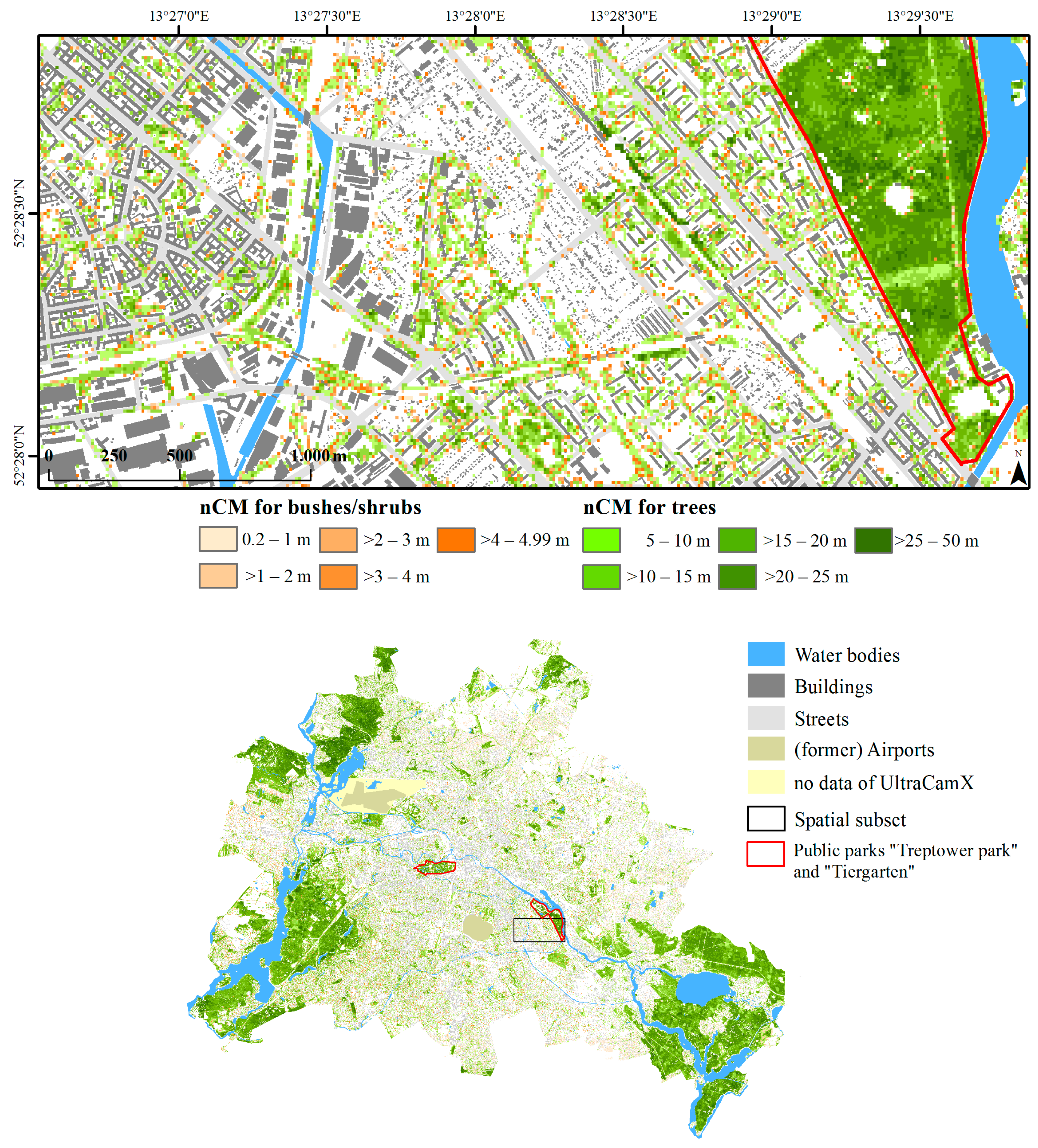
How are vegetation heights and vegetation height classes distributed across the city of Berlin and across the 12 different biotope classes?
(2)
What level of accuracy can be achieved for the vegetation height and biotope classes with the proposed approach?
This study presents a novel methodological workflow for the spatial analysis of large-area height models with three vegetation height classes (total vegetation, bushes and shrubs, trees). The results show different accuracies of CHMs for various urban vegetation settings derived by a TanDEM-X DEM in comparison to heights calculated by very high-resolution data. Moreover, this output informs about the interactions of the X-band with various urban vegetation structures. Besides methodological insights, the results also points out for the first time how vegetation heights are distributed across the city and across biotope type classes for the whole area of Berlin. Since this study aims to proof the capacities of the TanDEM-X DEM for urban vegetation height assessment on spatially explicit units, this study does not include the already existing very high resolution UltaCamX vegetation layer for assessment of vegetation heights on biotopes.

2. Materials and Methods

To address the outlined research questions, TanDEM-X intermediate DEM data were used along with the following additional datasets: a LiDAR digital terrain model (DTM), an UltraCamX vegetation height layer, and a biotope map (compare Table 1). Methods are described for two different vegetation height classes, bushes/shrubs and trees. A workflow based on techniques of data integration and raster algebra, including the following main steps, was applied: pre-processing of the TanDEM-X IDEM, processing of a mask for non-vegetated areas, CHM processing, CHM classification in two vegetation height classes (<4.99 m: bushes and shrubs; >5 m: trees), and derivation of vegetation heights for the 12 biotope classes of Berlin (compare Figure 1). Accuracy of the CHMs and biotope class heights are assessed using validation CHMs. An advanced method for non-vegetation masking was applied to improve vegetation area and height assessment. Unlike former approaches, the study does not aim to be particularly immanent of other data, but to include an additional LiDAR DTM to evaluate best possible height results for spatially explicit units. All steps were realized using the statistical software “R” (Version 3.2.0, packages “Raster, “rgdal”, “rgeos”, “kriging”; [40] and the GIS platform GQIS, Version 2.6.0, ”Brighton” [41]).

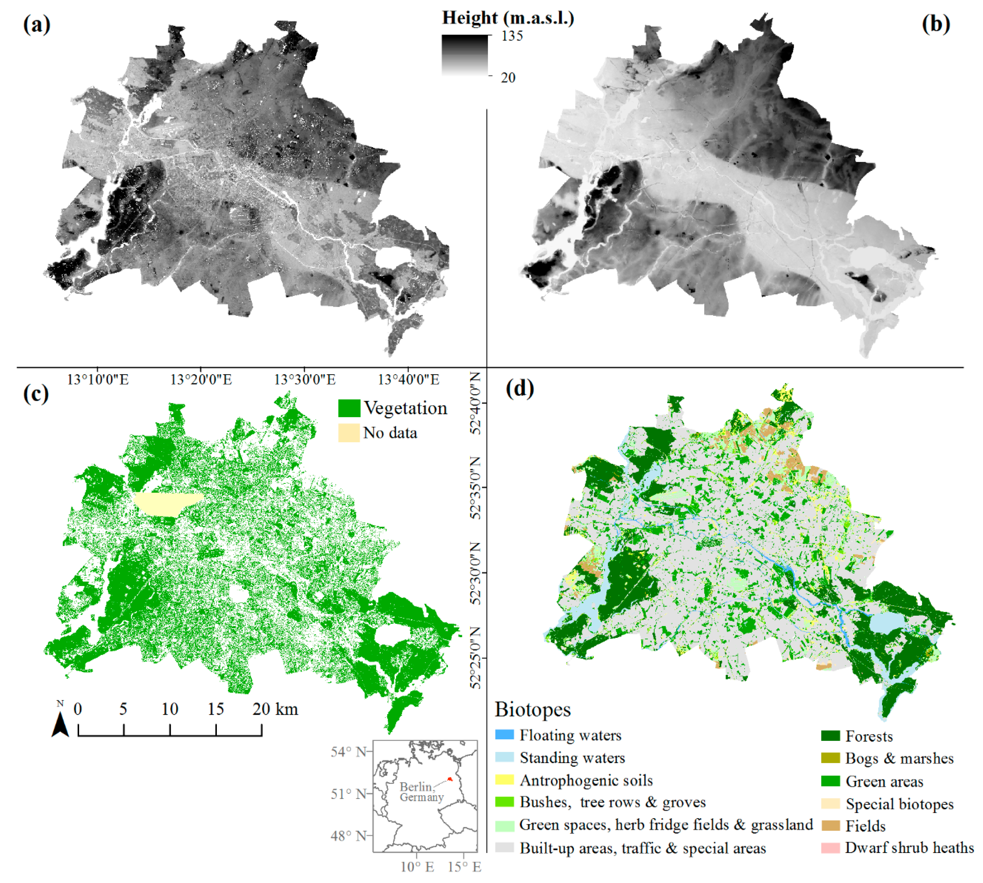
2.1. Study Area and Data

Situated in the northeast of Germany, and covering an area of ~892 km2, Berlin (λ 52°30′N, φ 13° 25′E; compare Figure 2) holds the largest amount of urban vegetation in absolute numbers (~356 km2) and highest number of urban dwellers (2012: ~3.5 M) within the country. Approximately 40% of the city area is covered by vegetation, which can be separated in stocks of typical forest-like (mainly commercial forests, public parks, and allotments) and typical urban-like conditions (mainly street trees, backyards, and green areas besides channels). The vegetation’s vertical structure is diverse as well, as a result of heterogeneous composition of types and species and stocks of different ages [44]. Additional information on the trees’ condition can be found in the Forest Conditions Report 2013 [45]. Due to the coverage of various vegetation types in different urban structures and, moreover, the provision of excellent validation height data, Berlin was chosen as a case study.
An intermediate DEM (IDEM) of the TanDEM-X mission (90.25% valid pixels, June 2012; leaf-on state of vegetation [46]) was available for this study. The IDEM is a product derived from acquisitions from the first coverage with one baseline configuration only and thus does not profit from dual-/multiple-baseline techniques and incidence angles. Especially, phase unwrapping errors may occur from missing additional acquisitions [47]. A DTM of the Official Topographical Cartographic Information System, derived from last-return pulses from airborne LiDAR data (August 2007), was combined with the IDEM for processing the height models (Table 1). A vegetation height layer from an airborne UltraCamX matrix camera was used for two purposes: the processing of a non-vegetation mask, and validating the CHMs. The vegetation layer is a photogrammetric product that was available as a shapefile from the Berlin Senate Department of Urban Development. It had been derived from very high resolution RGB and IR data by an UltraCamX matrix camera (Table 1). The IR data were used to identify the vegetated areas. The 12 biotope classes from the official biotope map of Berlin (Figure 2), which covers all of the Berlin area, were used for spatial analyses of the three produced CHMs for the entire vegetation, trees, and shrubs/bushes. The biotope classes of Berlin vary a lot in size, dominance of anthropogenic use, and vegetation types. The largest class is Built-up areas, traffic & special areas with the most sealed surface and street trees. In contrast, forests are (commercial) woodlands with a heterogeneous composition of vegetation species partially in near-naturally conditions. More detailed information on the biotopes’ definition and characteristics can be found in the environmental atlas of the senate administration of Berlin [22].

2.2. Pre-Processing

A pre-processed TanDEM-X IDEM was available for this study from a former approach [35] where the following steps had been applied: (a) conversion from ellipsoidal to orthometric heights to enable data integration, and (b) removal of random errors by water masking including the biotope map and a provided height error mask followed by local outlier detection using a method of Breunig and Kriegel [48]. For this study, the available LiDAR DTM (5 × 5 m) was resampled to the spatial resolution of the TanDEM-X data (12 × 12 m) by aggregating contiguous cells by bilinear interpolation. To gain a validation CHM, the UltraCamX vegetation layer was rasterized and attributed with the mean height. This raster was duplicated and thresholded in two single CHMs (bushes and shrubs: <4.99 m, trees: >5 m) to assess the height accuracy of the derived vegetation height classes from TanDEM-X. All data were available on the same grid size and in the same reference system.

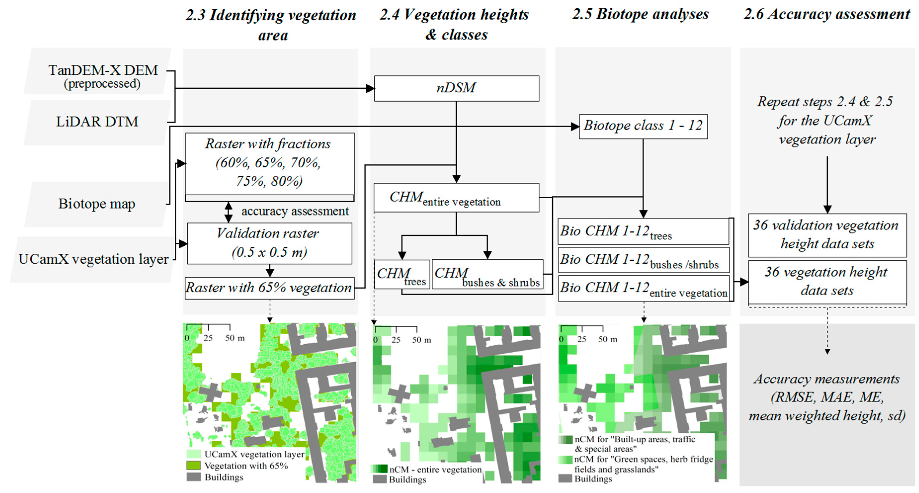
2.3. Identifying Vegetation Area

A non-vegetation mask was calculated to limit the following steps to those areas that were covered by vegetation. Because the pixel size of 12 × 12 m covers heights of vegetation and adjacent artificial objects, the vegetation had to be identified carefully. For this step the study relied on the UltraCamX vegetation layer that provides detailed vegetation information for the entire city of Berlin. The vegetation fraction of the vegetation layer (0–100%) was calculated for each 12 × 12 m grid cell of the TanDEM-X data using bilinear interpolation. Ten different vegetation rasters with fractions of 10%, 20%, …, 100% were computed. The resulting vegetation layers were then visually checked for overlapping with artificial objects using Open Street Map data of Berlin [49]. The Open Street Map data were chosen for an initial assessment in this study because they comprise detailed information on all urban objects, even though the data rely on several acquisition dates. Rasters with vegetation fractions of >80% lead to an inclusion of non-vegetation objects (errors of commission) and those with vegetation fractions of <60% to an exclusion of single vegetation components and small stocks (errors of omission). To identify the best suitable fraction, five rasters in the range of 60–80% with different vegetation fractions (60%, 65%, 70%, 75%, and 80%) were then calculated. The five rasters and a rasterized UltraCamX layer were disaggregated to a fine resolution of 0.5 × 0.5 m and converted to binary images (0: non-vegetation; 1: vegetation). Finally, the Overall Accuracy (OVA) and Cohen’s kappa coefficient were calculated for each vegetation raster and the disaggregated vegetation raster using confusion matrices [50]. Results demonstrated the best accuracy for a vegetation fraction of 65% (kappa: 0.69, OVA: 0.79). Accordingly, this raster was used as non-vegetation mask in the following step.

2.4. Vegetation Heights and Vegetation Height Classes

The height of an object on the earth’s surface can be estimated by subtraction of a digital terrain model (DTM) from a digital elevation model (DEM). The mathematical procedure of subtraction of two digital height models within the same geographical reference system is called normalization:
nDSM = DEM – DTM.
The result is a normalized digital height model (nDSM) in which the terrain is set to the standard of zero everywhere [51]. Then, it is possible to derive a canopy height model (CHM) by masking non-vegetation areas from the nDSM.
The derivation of rural and urban vegetation heights by the process of normalization is a well-established technique that has been often applied to LiDAR data [52,53,54]. Vegetation height classes, e.g., trees, bushes, and shrubs can be classified from the CHM by height ranges [13,14].
In this study, the LiDAR DTM was subtracted from the pre-processed TanDEM-X IDEM and all artificial and other natural urban objects were excluded using the non-vegetation mask. Even though the temporal difference of the LiDAR DTM and TanDEM-X DEM is about five years, the method was applied since a terrain model is less prone to changes than a height model covering urban objects. Next, the CHM was separated into vegetation height classes bushes and shrubs (<5 m) and trees (≥5 m). The thresholds are based on the height assumptions of Kang, Minor, Park and Lee [14], who derived urban vegetation height classes in the following manner: 1 to 5 m = shrubs; >5 m = trees. Since bush species also cover a height range up to 5 m [55], the classes bushes and shrubs were combined and the lower bound was set to 0.20 m in this study. An additional height class <0.20 m including lawns was not thresholded because the accuracy of the CHM for the total vegetation only allows for a very scattered assessment of this vegetation with low heights. This is known to be mainly caused by reflection of the X-band on the surface of less dense small objects, such as wheat fields and lawns [56].
The vertical division in both vegetation height classes can be based on different classifications, for example, combining the classes tree and shrub [57] or changing thresholds, as did Pellissier, Cohen, Boulay and Clergeau [13], who consider the lower class bound for trees at 10 m.

2.5. Vegetation Heights for Biotope Classes

Layers of the biotope classes intersected with each one of the three CHMs, namely, for the total vegetation, bushes and shrubs, and trees, to extract 36 single layers containing the respective vegetation heights for all 12 biotope classes. The separation into single files was necessary due to processing capacities. Because multiple polygons of the 12 biotope class layers jointly cover single grid cells of the CHMs, the fraction for the coverage of each CHM pixel was calculated as well. Overall, ~30% of all pixels were not fully occupied by the layer including the biotope classes. To take this into account, the calculated fractions were used as weights for the height and area calculation of vegetation for each biotope class. Consequently, the weighted mean vegetation heights for every vegetation height class and biotope class (m) as well as the weighted area size (m2) were calculated.

2.6. Accuracy Assessment

To assess the accuracy of all CHMs and the heights for 12 biotope classes, the respective validation datasets for accuracy assessment were calculated using the rasterized UltraCamX data (=the validation CHM) repeating the same steps of vegetation height assessment as for the TanDEM-X data. Overall, three validation CHMs for the vegetation height classes and 36 validation sheets (12 for every biotope class) containing the heights of every extracted CHM raster pixel were set against the corresponding outcome. This procedure did not include LiDAR data because the available LiDAR DEM did not cover the complete study area (~78%, compare [4]) and had a difference in time of data acquisition of >5 years compared to the TanDEM-X DEM.
Vertical offsets were assessed by the root-mean-square error (RMSE), the mean absolute error (MAE) and the mean error (ME), which are common measurements in accuracy assessment of height models [33,58]. The RMSE is the square root of the variance between the pre-processed and the validation DEM, and provides information about the occurrence of large deviations, such as statistical outliers. In contrast, the MAE is the arithmetic mean of all absolute height differences and does not emphasize large offsets. The ME is a mean value representing the actual positive or negative offset [59]. The mean heights, quantiles and standard deviations (σ) were calculated for the three vegetation height classes, and the corresponding validation models, to compare the height distribution.

3. Results

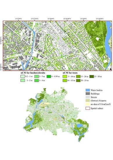
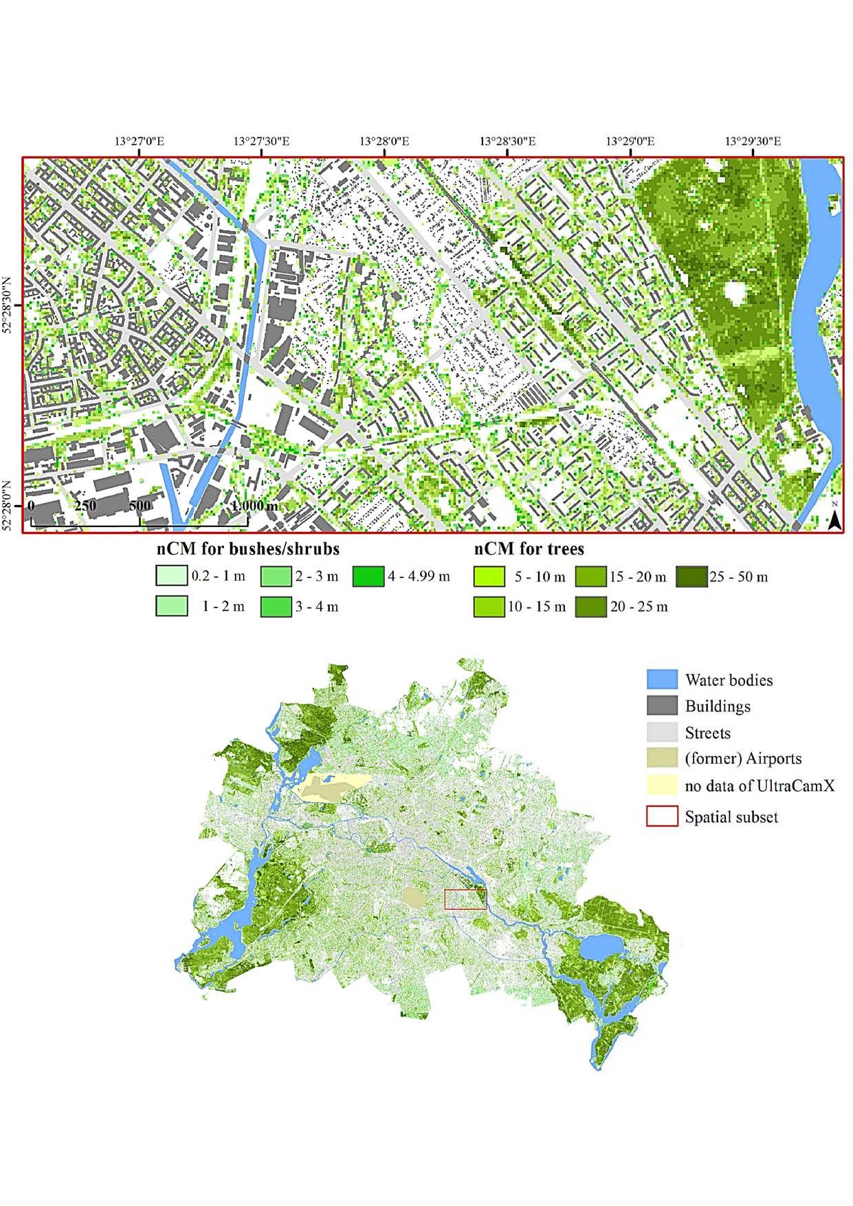
3.1. Vegetation Heights

Area-wide CHM and CHMs for two vegetation height classes (shrubs/bushes and trees) were obtained. Both CHMs are displayed with a building layer made using the UltraCamX data in Figure 3, which shows the spatial distribution of both vegetation height classes throughout Berlin. The urban-rural gradient of both, vegetation areas and vegetation heights, are clearly depicted. The densely built-up city center is mostly occupied by small stocks and individuals of both vegetation height classes; and partly interrupted by public parks and cemeteries with old and high tree stock (e.g., the public parks Tiergarten and Treptower Park, Figure 3). Large densely forested areas with high stock >20 m are located in the surrounding of lakes and inflows in the eastern and western part of the city.
The subset in Figure 3 shows a heterogeneous area with mixed residential, industrial and traffic use. It has different arrangements of both vegetation height classes on public and private space. As a result of the masking of non-vegetated areas, both CHMs do not cover neighboring buildings with few exceptions. Bushes and shrubs display an increased occurrence at the border of areas covered with linear arrangements of trees, such as channels.

3.2. Accuracy Assessment of Vegetation Heights

The assessed accuracies of the vegetation heights are summarized in Table 2, which shows the mean heights, quantiles, standard deviations, and height model deviations (RMSE, MAE, ME) for the CHMs of all vegetation height classes processed by the TanDEM-X and LiDAR data and the corresponding validation data derived by the UltraCamX vegetation layer. The comparison reveals an underestimation of mean heights for the total vegetation, and for trees as well (TanDEM-X CHM: 10.46 m; validation CHM: 12.02 m; TanDEM-X CHM for trees: 13.17 m; validation CHM for trees: 15.40 m). In comparison to an earlier study on urban vegetation height assessment [35], the results could be significantly improved (for the earlier study: mean height of 6.66 m for total vegetation in a subset of ~70 km2). Contrarily, the mean height for bushes/shrubs from the TanDEM-X CHM is larger than the validation height with 2.90 compared to 2.29 m.
The distribution of the quantiles for CHMs for the total vegetation and trees indicates a constant offset to the validation heights, with similar deviations of the 50% and 75% quantiles (~2.25 m). The RMSE, MAE, and ME for the CHMs for total vegetation and trees are higher than for bushes/shrubs, indicating a large range of values. Equivalently, the greatest standard deviations are measured in the CHM for all vegetation, followed by the one for trees and for bushes and shrubs (Table 2). For all validation models of the UltraCamX, the standard deviations were calculated to be higher than the TanDEM-X CHMs.

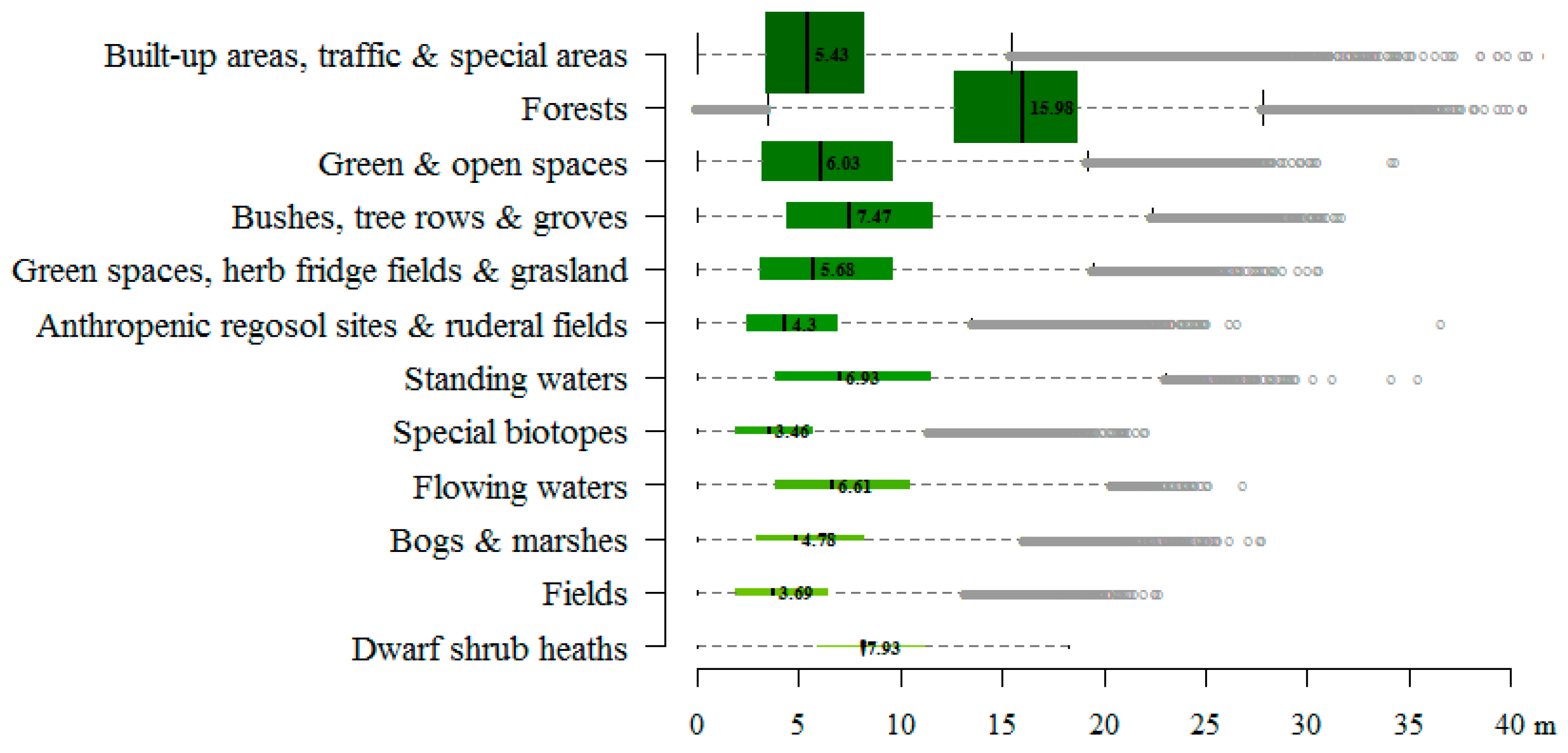
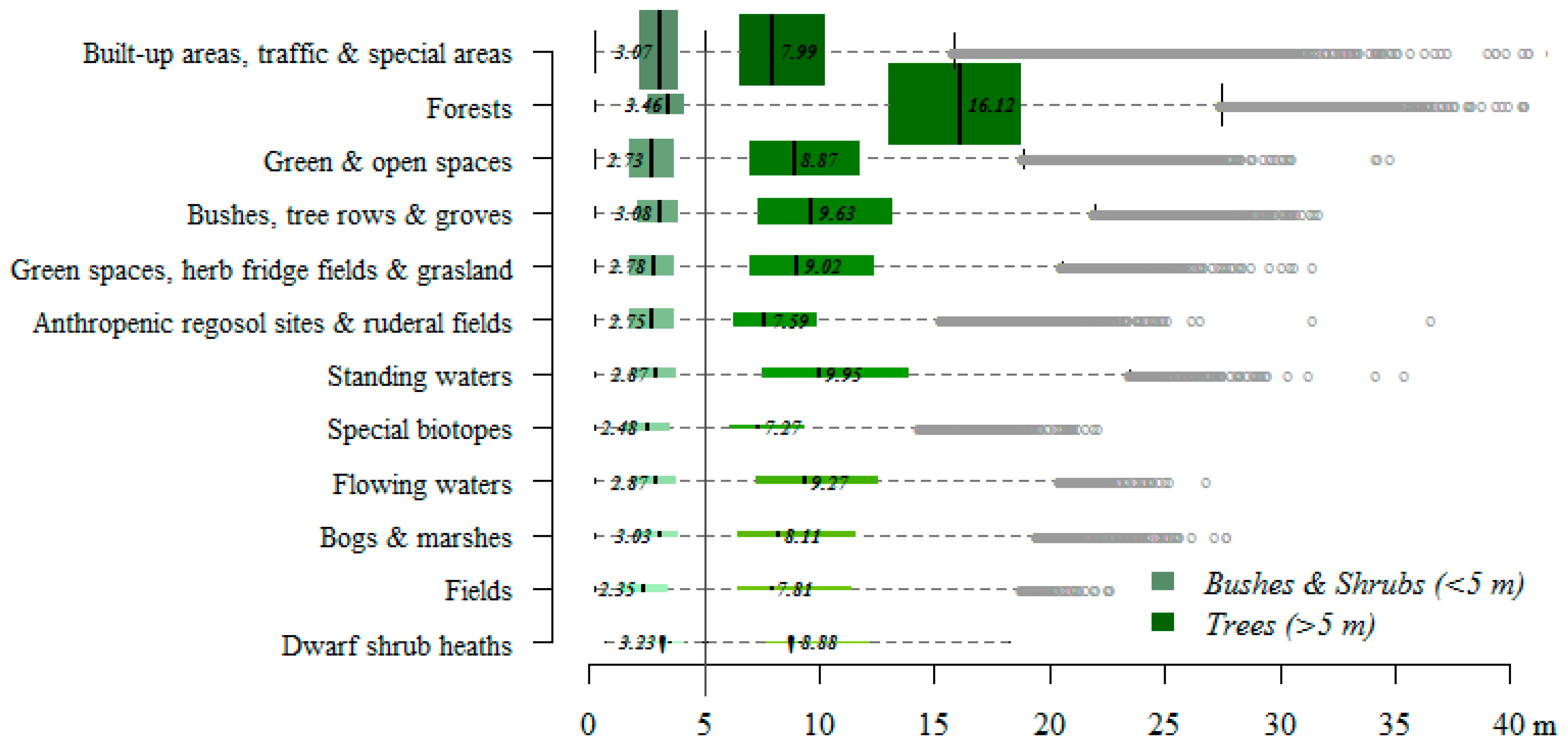
3.3. Vegetation Heights and Areas across Biotope Classes

Figure 4 and Figure 5 show boxplots of vegetation heights on the 12 biotope classes for the total vegetation, trees, and bushes/shrubs. Table 3, Table 4 and Table 5 (Section 3.4) include the absolute coverage and fraction of the total vegetation, trees, and bushes/shrubs on each biotope class. In the following, results for vegetation height and area are presented jointly, first for the total vegetation and then for trees and bushes/shrubs.
The median height of the total vegetation for all biotope classes appear to differ greatly, ranging from ~3.50 m up to ~16.00 m (Figure 4 and Figure 5). Summed up, 447.45 km2 (~42%) of all biotope classes are covered with vegetation (excluding lawns) with large differences within each biotope class for the total vegetated area (0.04–197.26 km2) and the vegetation fraction (4.44%–96.53%) (Table 3, Table 4 and Table 5, Section 3.4).
The biotope-related results show that the city’s vegetation is dominated by the vegetation height class “trees.” As expected, the two biotope classes Forests and Bushes, tree rows, and groves holds the largest weighted mean vegetation heights (in the following, the weighted mean vegetation height is also referred to as “μ”), and are covered by vegetation the most (>90%). The biotope class Forests is the only one with a weighted mean height >10 m and clearly holds the tallest vegetation (median: 15.98 m; μ: 15.78 m). Of particular note are Built-up areas, traffic, and special areas that hold the largest amount of vegetated area (197.26 m2, ~42% vegetation of biotope class), but small median (5.43 m) and weighted mean (6.07 m) heights, as well as a less distributed range of values. Surprisingly, the water-dominated biotope classes Standing waters (μ: 8.29 m) and Flowing waters (μ: 8.03 m) comprise tall vegetation; however, their fractions of vegetated area are listed among the lowest. The biotope class with the lowest weighted mean height is Special biotopes (μ: 3.97 m).
Overall, 322.03 km2 (~36%) are covered with trees and 137.87 km2 (~15.5%) with bushes and shrubs. All biotope classes hold a larger total amount of trees than bushes and shrubs, with few exceptions (e.g., Anthropogenic regosol sites and ruderal fields). The tree heights are similarly distributed on biotope classes like the total vegetation, while heights of bushes and shrubs follow a different pattern (Table 4 and Table 5). Concerning bushes and shrubs, the biggest total area (88.46 km2) and second tallest weighted mean height (μ: 2.97 m) appear to be in class Built-up areas, traffic & special areas, whereas Bogs & marshes (39.42%) is the class with the highest fraction.

3.4. Accuracy Assessment of Biotope Classes

For accuracy assessment of vegetation heights on biotope classes, the statistical height deviations to the validation data (RMSE, MAE, and ME) and the weighted mean heights of results and validation data (in the following also referred as “μVal”) were compared for the total CHM (Table 3) and both additional vegetation height classes (Table 4 and Table 5).
For the total vegetation, the accuracy revealed a positive to a negative offset to the validation CHMs with increasing vegetation heights (μ-μVal: −1.78 m to 4.23 m, Table 3). Biotope classes Forests and Bushes, tree rows, and groves hold taller vegetation than the corresponding validation unit (expressed as a negative value), which are also the ones occupied by more than 90% by vegetation. For the other biotope classes the heights appear to differ between ~1.00 m (Bogs and marshes) and >4.00 m (fields; dwarfs shrub heaths; green space; herb fridge fields and grassland; standing water). Most of the positive offsets larger than 4 m exist in biotope classes with vegetation fractions lower or similar to 25%.
For the trees and bushes/shrubs, all validation weighted mean heights are higher for trees (μ-μ Val: −2.01, compare Table 4) and all are lower for bushes and shrubs (μ-μVal: 0.51, compare Table 5). These relationships are the same as for the three CHMs that are not separated into biotope classes (Section 3.2).

4. Discussion

The vegetation height classes are distributed across the study area according to site-specific knowledge about the characteristics of Berlin’s street trees [44] and forested areas [45]. However, the thresholding procedure of delineating bushes/shrubs and trees likely causes a mixture of both classes in the height range close to the threshold value of 5.00 m. False classifications may arise in areas of large tree crowns ranging beyond 5.00 m, which is probably the reason for the presence of bushes and shrubs along linearly arranged tree stocks in Section 3.1. The CHM for bushes and shrubs is highly underrepresented in the sub-canopy layer of dense tree stocks, because the TanDEM-X DEM represents heights of the above-canopy layer only and does not reveal information about the layer underneath. Reliable sub-canopy information could additionally be derived by airborne LiDAR with a high point-cloud density [62], ground-based LiDAR data [63,64], or InSAR measurements using the L-Band [65], which was not available for this study.
For the results on height and biotope classes, the exclusion of non-vegetation objects was crucial for the metrics on vegetation area and height. Overall, the identified vegetation areas are “conservative” estimates of the actual distributions, because the procedure aimed to constantly reduce errors of commissions (overestimation of vegetated area) by taking into account a higher rate for errors of omission (underestimations of vegetated area). As a consequence, the resulting vegetation raster of the UltraCamX data excluded all vegetated area within the nDSM, where the vegetation coverage of each pixel was less than 35%. Single components with a small crown were removed, for example smaller species in allotment gardens and ornamental trees as wells as larger vegetation-covered areas that spanned across several pixels but had a small fraction (<35%) within each cell. Nevertheless, remaining vegetation heights in the respective CHMs can be considered to be correct. The errors of omission are likely to be high in densely vegetated biotope classes with many trees such as Forests, while they are lower in classes occupied by single or less dense vegetation components, such as Built-up areas & traffic and special areas or Bogs and marshes.
In comparison to studies using other remote sensing height data for vegetation height assessment, the accuracies in terms of the RMSE are very promising (Total Vegetation: 5.02 m, bushes/shrubs: 1.73 m, trees: 4.62 m). Liu, et al. [66] used SRTM data (30 × 30 m) for vegetation height extraction in rural forest areas, and identified a mean RMSE of ~19.00 m for two test sites. Imai, Setojima and Yamagishi [28] compared airborne LiDAR data with 1 m and 2 m resolutions for tree height assessment and gained RMSEs ranging from 2.72 m to 8.58 m.
However, the observed offset to the validation data for the single vegetation height classes (TanDEM-X total CHM/total val CHM: 10.46/12.02 m; TanDEM-X CHM for trees/val CHM for trees: 13.17/15.40 m, TanDEM-X CHM for bushes and shrubs/val CHM for bushes and shrubs: 2.90/2.29 m), has several potential reasons. As mentioned in the beginning, the height results have to be interpreted against the background of the interaction of X-bands and canopies in forest structures. Recent studies identified varying accuracies depending on stock density, height, and species composition: Balzter, et al. [67] compared TanDEM-X IDEM heights with heights by resampled airborne LiDAR for a very dense forest and found that both sensors’ scattering phases center in the canopy but for the TanDEM-X data at a lower position than for the LiDAR data. Izzawati Izzawati, Wallington and Woodhouse [36] proved a wave penetration up to several meters, which alters with varying degrees of plantation density and tree height. Perko, Raggam, Deutscher and al. [37] compared TerraSAR-X and COSMO-SkyMed and measured for both sensors a systematic height underestimation of a dense forest mainly dominated by deciduous trees (TerraSAR-X: 20–25%, COSMO-SkyMed: 20%). Solberg, Astrup, Bollandsas and al. [38] normalized a SRTM DEM by an airborne LiDAR DTM for forest structures and stated a vast underestimation as well, especially for trees <4 m in less dense forest stocks. Such a general underestimation of tree heights with X-band sensors is found in this study in the underestimation of the height class “tree” of about 2.23 m and a deviation of mean heights of about 1.56 m of the total vegetation compared to the validation data.
For the CHM of height class “bushes and shrubs”, mean heights are 0.61 m above the ones for the validation CHM. Since the mentioned studies on X-band–canopy interaction prove decreasing negative deviations with decreasing vegetation heights, other reasons have to be taken into account. A potential cause for the offset is the intermediate status of the TanDEM-X DEM, in which values are calculated from the first sensor coverage with one baseline configuration only, and false depictions of the actual heights are highly probable [46,68]. The quality of height values will be improved in the upcoming final DEM product due to multiple acquisitions and improved processing techniques [69], which will likely ameliorate height values in the CHM product as well. Another source of false CHM values may be routed in the fusion of multi-temporal data products, which leads to a potentially false identification of vegetation objects using the UltraCamX layer and the normalized IDEM. However, the temporal differences are reduced to the years 2010 (UltraCamX vegetation layer), 2012 (Biotope map & TanDEM-X IDEM and related height error mask) and 2014 (LiDAR DTM). All products were carefully compared concerning their spatial position and orthorectified to the TanDEM-X DEM.
Since the workflow is sequential, the results of the biotope-related analyses are affected by the previously derived CHMs, and the discussed problems have to be taken into account. For all biotope classes, height accuracies seem to depend on the vegetation’s mean height and on the fraction of vegetated area. For the height models with total vegetation and trees, biotope classes with widespread and tall vegetation have a constant offset about −2 m to the validation heights; the offset of biotopes with smaller vegetation height and area ranges between 0.26 and 0.83 m. In relatively small and generally treeless biotope classes, such as dwarf shrub heaths or fields, the heights deviate up to 4 m from the corresponding validation heights. These conditions point to the abovementioned relations of variances in different vegetation structures in X-band based height assessments. However, results for biotopes with a small vegetation fraction for Berlin have to be examined critically, because the low number of investigated vegetated pixels in these classes represents a small basis for statistical metrics.
The whole approach can be applied with less effort to other urban areas if terrain models and vegetation data are available. For several countries and urban areas LiDAR DTMs exist or are currently conducted, for example for Sweden with 1 m resolution on the national level [70]. The fractionated non-vegetation mask can be replaced using multispectral RapidEye (5.00; BlackBridgeAG [71]), Quickbird data (0.65 m; DigitalGlobe [72]) or the free and globally available multispectral images of the Sentinel-2 mission (10 m; (Gatti and Bertolini [73]). Even more, the use of additional vegetation information for non-vegetation masking can be avoided by classification of the TanDEM-X InSAR data, e.g., by using the coherence loss caused by volume scattering that is mainly caused by the presence of vegetation [39]. Moreover, more future efforts on the accurate deviation on DTMs by the TanDEM-X DEM would strengthen the data immanence and transferability of the approach.
In order to extract single trees of a 12 × 12 M CHM, their number could be approached by allometric assumptions. For instance, Pretzsch, et al. [74] investigated several species of ~39,000 urban trees from nine worldwide metropolitan areas and averaged the crown area for three tree height classes. Using this background, the number of single trees within a CHM for trees could be approximated by relating the height specific crown area and the pixel size

5. Conclusions

This study tested a globally available TanDEM-X DEM to assess spatially explicit urban vegetation heights for the entire city of Berlin, Germany. Applied methods comprised techniques of raster algebra and data integration, which sought to ameliorate results of former approaches for vegetation heights, and a clear delineation of urban vegetation and artificial objects. Similar to other studies dealing with height measurements of forest structures with X-band InSAR, the accuracy assessment revealed an underestimation of mean heights for total vegetation and trees; contrarily, the height for bushes was found to be above the validation height. The same relationships were identified for the three vegetation height classes on the 12 biotope classes. The vegetation height accuracies on biotope classes provide crucial information about height accessibility for different urban land use classes using a TanDEM-X driven approach.
The use of TanDEM-X data for vegetation assessment can be recommended for other urban areas, since they have great accuracies that complement high-resolution data. For integrating TanDEM-X CHMs, future studies have to invest in realizing the value of ecosystem services and cost assessment as single height values or metrics on a composite of heights. In this manner, standard deviations could be used as a parameter for measuring the heterogeneity of specific areas and height classes. The number of single trees could be approached by allometric assumptions. The results would open up a wide range of applications of vegetation height and area information for ecosystem service studies on different height classes, spatial units (e.g., biotope classes or other land use classes) and spatial scales (e.g., urban subsets, entire cities, or metropolitan areas), solely or in addition to species and age information on vegetation. Potential contributions could be made on nearly all large-area approaches of vegetation-related services that currently use area information only, for example for city-wide biomass and carbon assessments [20,75] or climate mitigation studies [76]. Overall, the final TanDEM-X DEM could contribute greatly to vegetation-related ecosystem studies, taking into account the reliability of single vegetation height classes and their heights on biotope classes.

Acknowledgments

This study is supported by the German Research Foundation (DFG) as part of graduate program 1324 “Model-Based Development of Technologies for Self-Organizing Decentralized Information Systems in Disaster Management” (METRIK). Costs to publish in open access were covered by the GIScience lab of Humboldt-Universität. We would like to thank the German Aerospace Center (DLR) for the provision of intermediate TanDEM-X data, and the Senate Administration of Berlin for providing the additional data products. Moreover, we would like to thank Florian Gollnow and Leticia Hissa for contributions to an earlier version of the manuscript.

Author Contributions

Johannes Schreyer developed the methodology, collected, processed, and analyzed the data, and wrote the paper. Tobia Lakes supervised the entire process and intensely contributed to manuscript constructing and writing.

Conflicts of Interest

The authors declare no conflict of interest.

References

  1. Escobedo, F.J.; Kroeger, T.; Wagner, J.E. Urban forests and pollution mitigation: Analyzing ecosystem services and disservices. Environ. Pollut. 2011, 159, 2078–2087. [Google Scholar] [CrossRef] [PubMed]
  2. Sandstrom, U.G.; Angelstam, P.; Mikusinski, G. Ecological diversity of birds in relation to the structure of urban green space. Landsc. Urban Plan. 2006, 77, 39–53. [Google Scholar] [CrossRef]
  3. Croci, S.; Butet, A.; Georges, A.; Aguejdad, R.; Clergeau, P. Small urban woodlands as biodiversity conservation hot-spot: A multi-taxon approach. Landsc. Ecol. 2008, 23, 1171–1186. [Google Scholar] [CrossRef]
  4. Tigges, J.; Lakes, T.; Hostert, P. Urban vegetation classification: Benefits of multitemporal RapidEye satellite data. Remote Sens. Environ. 2013, 136, 66–75. [Google Scholar] [CrossRef]
  5. Bergen, K.M.; Goetz, S.J.; Dubayah, R.O.; Henebry, G.M.; Hunsaker, C.T.; Imhoff, M.L.; Nelson, R.F.; Parker, G.G.; Radeloff, V.C. Remote sensing of vegetation 3-D structure for biodiversity and habitat: Review and implications for LiDAR and Radar spaceborne missions. J. Geophys. Res. Biogeosci. 2009, 114, G00E06. [Google Scholar] [CrossRef]
  6. Lehmann, I.; Mathey, J.; Rößler, S.; Bräuer, A.; Goldberg, V. Urban vegetation structure types as a methodological approach for identifying ecosystem services—Application to the analysis of micro-climatic effects. Ecol. Indic. 2014, 42, 58–72. [Google Scholar] [CrossRef]
  7. Roy, S.; Byrne, J.; Pickering, C. A systematic quantitative review of urban tree benefits, costs, and assessment methods across cities in different climatic zones. Urban For. Urban Green. 2012, 11, 351–363. [Google Scholar] [CrossRef]
  8. Schreyer, J.; Tigges, J.; Lakes, T.; Churkina, G. Using Airborne LiDAR and QuickBird Data for Modelling Urban Tree Carbon Storage and Its Distribution—A Case Study of Berlin. Remote Sens. 2014, 6, 10636–10655. [Google Scholar] [CrossRef]
  9. Johnson, A.D.; Gerhold, H.D. Carbon storage by urban tree cultivars, in roots and above-ground. Urban For. Urban Green. 2003, 2, 65–72. [Google Scholar] [CrossRef]
  10. Lindberg, F.; Grimmond, C.S.B. The influence of vegetation and building morphology on shadow patterns and mean radiant temperatures in urban areas: Model development and evaluation. Theor. Appl. Climatol. 2011, 105, 311–323. [Google Scholar] [CrossRef]
  11. Ko, Y.K.; Lee, J.H.; McPherson, E.G.; Roman, L.A. Long-term monitoring of Sacramento Shade program trees: Tree survival, growth and energy-saving performance. Landsc. Urban Plan. 2015, 143, 183–191. [Google Scholar] [CrossRef]
  12. Jang, H.S.; Lee, S.C.; Jeon, J.Y.; Kang, J. Evaluation of road traffic noise abatement by vegetation treatment in a 1:10 urban scale model. J. Acoust. Soc. Am. 2015, 138, 3884–3895. [Google Scholar] [CrossRef] [PubMed]
  13. Pellissier, V.; Cohen, M.; Boulay, A.; Clergeau, P. Birds are also sensitive to landscape composition and configuration within the city centre. Landsc. Urban Plan. 2012, 104, 181–188. [Google Scholar] [CrossRef]
  14. Kang, W.; Minor, E.S.; Park, C.R.; Lee, D. Effects of habitat structure, human disturbance, and habitat connectivity on urban forest bird communities. Urban Ecosyst. 2015, 18, 857–870. [Google Scholar] [CrossRef]
  15. Bertram, C.; Rehdanz, K. The Role of Urban Green Space for Human Well-Being; Kiel Institute for the World Economy: Kiel, Germany, 2014. [Google Scholar]
  16. Stagoll, K.; Lindenmayer, D.B.; Knight, E.; Fischer, J.; Manning, A.D. Large trees are keystone structures in urban parks. Conserv. Lett. 2012, 5, 115–122. [Google Scholar] [CrossRef]
  17. Donovan, G.H.; Prestemon, J.P. The Effect of Trees on Crime in Portland, Oregon. Environ. Behav. 2012, 44, 3–30. [Google Scholar] [CrossRef]
  18. Heisler, G.M. Effects of individual trees on the solar radiation climate of small buildings. Urban Ecol. 1986, 9, 337–359. [Google Scholar] [CrossRef]
  19. Cariñanos, P.; Casares-Porcel, M.; Quesada-Rubio, J.-M. Estimating the allergenic potential of urban green spaces: A case-study in Granada, Spain. Landsc. Urban Plan. 2014, 123, 134–144. [Google Scholar] [CrossRef]
  20. Strohbach, M.W.; Haase, D. Above-ground carbon storage by urban trees in Leipzig, Germany: Analysis of patterns in a European city. Landsc. Urban Plan. 2012, 104, 95–104. [Google Scholar] [CrossRef]
  21. Weber, N.; Haase, D.; Franck, U. Zooming into temperature conditions in the city of Leipzig: How do urban built and green structures influence earth surface temperatures in the city? Sci. Total Environ. 2014, 496, 289–298. [Google Scholar] [CrossRef] [PubMed]
  22. SenStadt. Environmental Atlas of Berlin—05, Biotope; Senate Administration of Berlin: Berlin, Germany, 2012.
  23. Büttner, G.; Kosztra, B.; Maucha, G.; Pataki, R. Implementation and Achievements of CLC2006; Institute of Geodesy, Cartography and Remote Sensing, Universitat Autònoma de Barcelona: Barcelona, Spain, 2012; pp. 1–65. [Google Scholar]
  24. Stewart, G.H.; Meurk, C.D.; Ignatieva, M.E.; Buckley, H.L.; Magueur, A.; Case, B.S.; Hudson, M.; Parker, M. Urban Biotopes of Aotearoa New Zealand (URBANZ) II: Floristics, biodiversity and conservation values of urban residential and public woodlands, Christchurch. Urban For. Urban Green. 2009, 8, 149–162. [Google Scholar] [CrossRef]
  25. Löfvenhaft, K.; Runborg, S.; Sjögren-Gulve, P. Biotope patterns and amphibian distribution as assessment tools in urban landscape planning. Landsc. Urban Plan. 2004, 68, 403–427. [Google Scholar] [CrossRef]
  26. Chisholm, R.A.; Cui, J.; Lum, S.K.Y.; Chen, C. UAV LiDAR for below-canopy forest surveys. J. Unmanned Veh. Syst. 2014, 1, 61–68. [Google Scholar] [CrossRef]
  27. Hecht, R. Development of a Method for Estimation of Urban Green Volume Based on Laserscanning Data in Leafy State [Entwicklung Einer Methode zur Erfassung des Städtischen Grünvolumens auf Basis von Laserscannerdaten Laubfreier Befliegungszeitpunkte]. Diploma Thesis, Technical University of Dresden, Dresden, Germany, 2006. [Google Scholar]
  28. Imai, Y.; Setojima, M.; Yamagishi, M. Tree-height measuring characteristics of urban forests by LiDAR data different in resolution. In Proceedings of the XXth ISPRS Congress, Istanbul, Turkey, 12–23 July 2004; pp. 513–516.
  29. Luederitz, C.; Brink, E.; Gralla, F.; Hermelingmeier, V.; Meyer, M.; Niven, L.; Panzer, L.; Partelow, S.; Rau, A.-L.; Sasaki, R.; et al. A review of urban ecosystem services: Six key challenges for future research. Ecosyst. Serv. 2015, 14, 98–112. [Google Scholar] [CrossRef]
  30. Krieger, G.; Moreira, A.; Fiedler, H.; Hajnsek, I.; Werner, M.; Younis, M.; Zink, M. TanDEM-X: A satellite formation for high-resolution SAR interferometry. IEEE Trans. Geosci. Remote Sens. 2007, 45, 3317–3341. [Google Scholar] [CrossRef]
  31. Huber, M.; Gruber, A.; Wendleder, A.; Wessel, B.; Roth, A.; Schmitt, A. The global TanDEM-X DEM: Production status and first validation results. In Proceedings of the XXII Isprs Congress, Technical Commission VII, Melbourne, Australia, 25 August–1 September 2012; pp. 45–50.
  32. Mäkelä, H.; Pekkarinen, A. Estimation of forest stand volumes by Landsat TM imagery and stand-level field-inventory data. For. Ecol. Manag. 2004, 196, 245–255. [Google Scholar] [CrossRef]
  33. Geiß, C.; Wurm, M.; Breunig, M.; Felbier, A.; Taubenböck, H. Normalization of TanDEM-X DSM Data in Urban Environments with Morphological Filters. IEEE Trans. Geosci. Remote Sens. 2015, 53, 4348–4362. [Google Scholar] [CrossRef]
  34. Marconcini, M.; Marmanis, D.; Esch, T.; Felbier, A. A novel method for building height estimation using TanDEM-X data. In Proceedings of the 2014 IEEE International Geoscience and Remote Sensing Symposium (Igarss), Quebec City, QC, Canada, 13–18 July 2014; pp. 4804–4807.
  35. Schreyer, J.; Geiß, C.; Lakes, T. TanDEM-X for Large-Area Modeling of Urban Vegetation Height: Evidence from Berlin, Germany. IEEE J. Sel. Top. Appl. Earth Observ. Remote Sens. 2016, 9, 1–12. [Google Scholar] [CrossRef]
  36. Izzawati; Wallington, E.D.; Woodhouse, I.H. Forest height retrieval from commercial X-band SAR products. IEEE Trans. Geosci. Remote Sens. 2006, 44, 863–870. [Google Scholar] [CrossRef]
  37. Perko, R.; Raggam, H.; Deutscher, J.; Gutjahr, K.; Schardt, M. Forest Assessment Using High Resolution SAR Data in X-Band. Remote Sens. 2011, 3, 792–815. [Google Scholar] [CrossRef]
  38. Solberg, S.; Astrup, R.; Bollandsas, O.M.; Næsset, E.; Weydahl, D.J. Deriving forest monitoring variables from X-band InSAR SRTM height. Can. J. Remote Sens. 2010, 36, 68–79. [Google Scholar] [CrossRef]
  39. Martone, M.; Rizzoli, P.; Bräutigam, B.; Krieger, G. Forest Classification from TanDEM-X Interferometric Data by means of Multiple Fuzzy Clustering. In Proceedings of the 11th European Conference on Synthetic Aperture Radar (EUSAR), Hamburg, Germany, 6–9 June 2016; p. 6.
  40. RCoreTeam. R: A Language and Environment for Statistical Computing; R Foundation for Statistical Computing: Vienna, Austria, 2015. [Google Scholar]
  41. QGIS DevelopmentTeam. Quantum GIS Geographic Information System—Open Source Geospatial Foundation Project. 2015. Available online: http://planet.qgis.org/planet/tag/opensource/ (accessed on 10 November 2016).
  42. Optech. Gemini ALTM production sheet. Optech: Vaughan, Canada. 2008. Available online: http://airsensing.com/wp-content/uploads/2014/11/Airborne_Gemini.pdf (accessed on 10 November 2016).
  43. Vexcel. UltraCamX—Technical Specifications; Vexcel Imaging GmbH: Graz, Austria, 2009; p. 2. Available online: https://www.kasurveys.com/documents/ULTRACAM-Specs-UCX.pdf (accessed on 10 November 2016).
  44. Fietz, M.; Burger, H. Street Trees Status Report Berlin [Strassenbaum-Zustandsbericht Berliner Innenstadt 2010]; Senate Department for Urban Development of Berlin: Berlin, Germany, 2011.
  45. SenStadt. Forest Conditions Report of Berlin [Waldzustandsbericht Berlin]; Senate administration of Berlin, Senate Department for Urban Development and the Environment: Berlin, Germany, 2014.
  46. German Aerospace Center. TanDEM-X Ground Segment—DEM Products Specification Document; German Aerospace Center: Oberpfaffenhofen, Germany, 2013. [Google Scholar]
  47. Rizzoli, P.; Bräutigam, B.; Kraus, T.; Martone, M.; Krieger, G. Relative height error analysis of TanDEM-X elevation data. ISPRS J. Photogram. Remote Sens. 2012, 73, 30–38. [Google Scholar] [CrossRef]
  48. Breunig, M.M.; Kriegel, H.-P. LOF: Identifying density-based local outliers. SIGMOD Rec. 2000, 29, 93–104. [Google Scholar] [CrossRef]
  49. OpenStreetMap. Available online: www.openstreetmap.de (accessed on 1 February 2016).
  50. Lillesand, T.M.; Kiefer, R.W. Remote Sensing and Image Interpretation, 5th ed.; John Wiley & Sons: Hoboken, NJ, USA, 2004. [Google Scholar]
  51. Serra, J. Image Analysis and Mathematical Morphology; Academic Press: Orlando, FL, USA, 1984; p. 610. [Google Scholar]
  52. Huang, Y.; Yu, B.L.; Zhou, J.H.; Hu, C.L.; Tan, W.Q.; Hu, Z.M.; Wu, J.P. Toward automatic estimation of urban green volume using airborne LiDAR data and high resolution Remote Sensing images. Front. Earth Sci. 2013, 7, 43–54. [Google Scholar] [CrossRef]
  53. Hecht, R.; Meinel, G.; Buchroither, M. Estimation of urban green volume based on last pulse LiDAR data at leaf-off aerial flight times. In Proceedings of the 1st EARSeL Workshop of the SIG Urban Remote Sensing, Berlin, Germany, 2–3 March 2006; pp. 1–8.
  54. Hyyppä, J.; Hyyppä, H.; Litkey, P.; Yu, X.; Haggren, H.; Rönnholm, P.; Pyysalo, U.; Pitkänen, J.; Maltamo, M. Algorithms and methods of airborne laserscanning for forset measurements. Int. Arch. Photgramm. Remote Sens. Spat. Inf. Sci. 2004, 36, 82–89. [Google Scholar]
  55. Davies, Z.G.; Edmondson, J.L.; Heinemeyer, A.; Eake, J.R.; Gaston, K.J. Mapping an urban ecosystem service: Quantifying above-ground carbon storage at a city-wide scale. J. Appl. Ecol. 2011, 48, 1125–1134. [Google Scholar] [CrossRef]
  56. Baghdadi, N.; Holah, N.; Dubois, F.P.; Prévot, L.; Hosford, S.; Chanzy, A.; Dupuis, X.; Zribi, M. Analysis of X-Band Polarimetric Sar Data for The Derivation of The Surface Roughness Over Bare Agricultural Fields. In Proceedings of XXth ISPRS Congress—Technical Commission I, Stanbul, Turkey, 12–23 July 2004.
  57. Nowak, D.J.; Escobedo, F.J. Spatial heterogeneity and air pollution removal by an urban forest. Landsc. Urban Plan. 2009, 90, 102–110. [Google Scholar]
  58. Liu, X.Y. Airborne LiDAR for DEM generation: Some critical issues. Prog. Phys. Geogr. 2008, 32, 31–49. [Google Scholar]
  59. Wasklewicz, T.; Staley, D.M.; Reavis, K.; Oguchi, T. Digital Terrain Modeling. In Treatise on Geomorphology; Elsevier Inc.: Cambridge, MA, USA, 2013; pp. 130–161. [Google Scholar]
  60. Poznanska, A.M. Determination of Building and Vegetation Heights in the City of Berlin [Bestimmung von Gebäude- und Vegetationshöhen im Berliner Stadtgebiet]; Deutsches Zentrum für Luft- und Raumfahrt (DLR e. V.) Abteilung Sensorkonzepte und Anwendungen am Institut für Optische Sensorsysteme: Berlin, Germany, 2013; p. 79. [Google Scholar]
  61. Poznanska, A.M. Data Base: Urban and Environmental Information System (UEIS)-06.10 Building and Vegetation Heights (Edition 2014); Senate Department for Urban Development and the Environment: Berlin, Germany, 2014.
  62. Shreshta, R.; Wynne, R.H. Estimating Biophysical Parameters of Individual Trees in an Urban Environment Using Small Footprint Discrete-Return Imaging LiDAR. Remote Sens. 2012, 4, 484–508. [Google Scholar] [CrossRef]
  63. Edson, C.; Wing, M.G. Airborne Light Detection and Ranging (LiDAR) for Individual Tree Stem Location, Height, and Biomass Measurements. Remote Sens. 2011, 3, 2494–2528. [Google Scholar] [CrossRef] [Green Version]
  64. Wu, B.; Yu, B.L.; Yue, W.H.; Shu, S.; Tan, W.Q.; Hu, C.L.; Huang, Y.; Wu, J.P.; Liu, H.X. A Voxel-Based Method for Automated Identification and Morphological Parameters Estimation of Individual Street Trees from Mobile Laser Scanning Data. Remote Sens. 2013, 5, 584–611. [Google Scholar] [CrossRef]
  65. Hajnsek, I.; Kugler, F.; Lee, S.K.; Papathanassiou, K.P. Tropical-Forest-Parameter Estimation by Means of Pol-InSAR: The INDREX-II Campaign. IEEE Trans. Geosci. Remote Sens. 2009, 47, 481–493. [Google Scholar] [CrossRef]
  66. Liu, J.K.; Liu, D.S.; Alsdorf, D. Extracting Ground-Level DEM From SRTM DEM in Forest Environments Based on Mathematical Morphology. IEEE Trans. Geosci. Remote Sens. 2014, 52, 6333–6340. [Google Scholar]
  67. Balzter, H.; Baade, J.; Rogers, K. Validation of the TanDEM-X Intermediate Digital Elevation Model With Airborne LiDAR and Differential GNSS in Kruger National Park. IEEE Geosci. Remote Sens. Lett. 2016, 13, 277–281. [Google Scholar] [CrossRef]
  68. GermanAerospaceCenter. TanDEM-X—Application and Use [Tandem-X—Anwendung und Nutzung]; German Aerospace Center: Munich, Germany, 2014. [Google Scholar]
  69. Martone, M.; Bräutigam, B.; Rizzoli, P.; Gonzalez, C.; Bachmann, M.; Krieger, G. Coherence evaluation of TanDEM-X interferometric data. ISPRS J. Photogram. Remote Sens. 2012, 73, 21–29. [Google Scholar] [CrossRef]
  70. Lundgren, J.; Juni, O. Accuracy Control of Laser Data for the new National Elevation Model [Noggrannhetskontroll av Laserdata för ny Nationell Höjdmodell]. Master’s Thesis, University of Gävle, Department for Technology and Environment, Gävle, Sweden, 2010. [Google Scholar]
  71. BlackBridgeAG. RapidEye—Satellite Imagery Product Specifications; BlackBridge AG: Berlin, Germany, 2015; pp. 1–48. [Google Scholar]
  72. DigitalGlobe. Quickbird Data Sheet; DigitalGlobe: Westminster, CO, USA, 2014. [Google Scholar]
  73. Gatti, A.; Bertolini, A. Sentinel-2 Products Specification Document (PSD); Thales Alenia Space: Cannes, France, 2015; p. 496. [Google Scholar]
  74. Pretzsch, H.; Biber, P.; Uhl, E.; Dahlhausen, J.; Rötzer, T.; Caldentey, J.; Koike, T.; van Con, T.; Chavanne, A.; Seifert, T.; et al. Crown size and growing space requirement of common tree species in urban centres, parks, and forests. Urban For. Urban Green. 2015, 14, 466–479. [Google Scholar] [CrossRef]
  75. Churkina, G. Modeling the carbon cycle of urban systems. Ecol. Model. 2008, 216, 107–113. [Google Scholar] [CrossRef]
  76. Alavipanah, S.; Wegmann, M.; Qureshi, S.; Weng, Q.; Koellner, T. The Role of Vegetation in Mitigating Urban Land Surface Temperatures: A Case Study of Munich, Germany during the Warm Season. Sustainability 2015, 7, 4689–4706. [Google Scholar] [CrossRef]
Figure 1. Workflow for vegetation identification, height classification, biotope analyses, and accuracy assessment of results. Columns 2.3–2.6 refer to sub-headings in Section 2. The column ends of Section 2.3, Section 2.4 and Section 2.5 depict a spatial subset of the outcome for the respective steps. The spatial subset of Column 2.5 gives an example of two biotope classes. nDSM = normalized difference surface model; CHMtotal vegetation = canopy height model for the total vegetation , CHMtrees = canopy height model for trees, CHMbushes & shrubs = canopy height model for bushes and shrubs; Bio CHM and inferior characters: these acronyms address the CHM for the three studied vegetation height classes with the 12 biotope layers.
Remotesensing 08 00940 g001
Figure 2. (a) TanDEM-X intermediate DEM; (b) LiDAR DTM; (c) UltraCamX vegetation layer; (d) 12 biotope classes. Technical specifications are listed in Table 1.
Remotesensing 08 00940 g002
Figure 3. Classified CHMs for bushes and shrubs (light green) and trees (dark green) for all of Berlin, and a subset in the district Treptow-Köpenick. The included water bodies are derived from the biotope map; the buildings are extracted from an officially available building layer derived from the UltraCamX matrix camera during the same flight campaign as the vegetation assessment [60,61].
Remotesensing 08 00940 g003
Figure 4. Boxplots of vegetation height distribution for the total vegetation. The biotope classes are ordered by the weighted area size. The widths of the boxes are drawn proportionally to the square roots of the number of observations (pixels with vegetation) in each biotope class. The outliers for the height class “trees” are indicated by gray circles. The median values are drawn adjacent to the median line.
Remotesensing 08 00940 g004
Figure 5. Boxplots of vegetation height distribution for vegetation height classes “Bushes/Shrubs” and “Trees” on 12 biotope classes. The biotope classes are ordered by the weighted area size. The widths of the boxes are drawn proportional to the square-roots of the number of observations (pixels with vegetation) in each biotope class. The outliers for the height class “trees” are indicated by gray circles. The median values are drawn adjacent to the median line.
Remotesensing 08 00940 g005
Table 1. Data & specifications.
Imagery/Vector DataSpecifications
TanDEM-X products
Intermediate Digital Elevation Model (IDEM)
Height Error Mask
Sensorsingle-pass SAR interferometer
AcquiredJune 2012 (leaf-on)
Spatial resolution12 × 12 m (0.4 arcsec at equator)
Absolute horizontal accuracy (CE90) & vertical accuracy (LE90)<10.00 m
Relative vertical accuracy (90% linear point-to-point error)Not specified
Incidence angleNot specified for study region, typically an angle of 39°
Height of ambiguityNot specified
Height referenceWGS84-G1150 ellipsoid
Airborne LiDAR product [42]SensorALTM Gemini
Acquired2007/08 (updated June 2014)
Point density1 point/m2
Spatial resolution5 × 5 m
Absolute horizontal & vertical accuracy0.05–0.10 m
Wavelength1064 mm
Height referenceGerman Leveling Network 1992 (DHHN92)
UltraCamX product [43]
vegetation height layer
building height layer
SensorMatrix camera for panchromatic RGB, IR (9420 × 14430 pixel)
AcquiredAugust 2010 (leaf-on)
Absolute horizontal & vertical accuracy
Height reference
0.10 m
European Terrestrial Reference System (ETRS89)
Biotope mapSensor/data basisVarious RS data (e.g., digital Orthophotos, analogue CIR aerial image slides) & existing vector data
Acquired2001–2012
Table 2. Comparative statistics for all produced CHM and Validation CHM (Val CHM), measured in meters.
Height ModelMean HeightQuantilesσRMSEMEMAE
0%25%50%75%100%
Total Vegetation
CHM10.460.004.789.6715.8663.00 *6.445.02−1.583.75
Val CHM12.020.004.8912.3018.6054.69 *7.72
Bushes/Shrubs
CHM2.890.211.902.963.964.981.261.730.541.38
Val CHM2.290.211.112.053.454.981.37
Trees
CHM13.175.018.4613.0517.2849.94 *5.274.62−2.473.53
Val CHM15.405.0110.5515.8319.9349.90 *5.83
* Wrong height values for pixel, caused by incorrect masking of non-vegetation.
Table 3. Vegetated area (km2Veg, Veg %), Weighted mean vegetation heights (μ) and validation heights (μval) and height deviations to validation heights (RMSE, MAE, and ME in meters) for the total vegetation on 12 biotope classes.
Biotope ClassVegetated AreaMean Heights *Height Deviations
km2km2%μμValμ-μValRMSEMAEME
Forests168.44162.5996.5315.7817.56−1.786.094.69−1.62
Bushes, tree rows, & groves18.8817.0190.129.0210.38−1.376.104.69−1.19
Bogs & marshes1.371.0576.535.574.580.995.734.080.24
Green & open spaces87.4145.9052.516.924.722.205.714.340.30
Built-up areas, traffic, & special areas473.59197.2641.656.074.141.925.644.411.34
Special biotopes3.661.4639.913.972.341.634.433.290.63
Anthropogenic regosol sites & ruderal fields21.477.3434.194.832.302.534.833.681.34
Green spaces, herb fridge fields, & grassland41.2410.4825.416.542.204.346.545.092.09
Dwarf shrub heaths0.180.0422.737.943.604.334.823.631.93
Flowing waters9.531.3514.168.035.302.746.204.840.46
Standing waters45.382.054.528.294.134.166.805.251.81
Fields20.720.924.444.570.354.235.113.882.74
μ41.892.16
* The mean heights are weighted with the fractions of each biotope class layer on the pixels of the respective CHMs.
Table 4. Area with trees (km2Veg, trees %), Weighted mean vegetation heights (μ) and validation heights (μVAL) and height deviations to validation heights (RMSE, MAE, and ME in meters) for trees in 12 biotope classes.
Biotope ClassArea with TreesMean Heights *Height Deviations
km2km2%μμValμ-μValRMSEMAEME
Forests168.44159.4894.6816.0618.33−2.273.822.92−2.23
Bushes, tree rows, & groves18.8813.2970.3911.0113.59−2.584.743.65−3.01
Bogs & marshes1.370.5137.238.9810.09−1.114.223.07−2.10
Green & open spaces87.4128.0032.039.9512.72−2.775.073.99−3.22
Built-up areas, traffic, & special areas473.59108.8022.978.7811.17−2.394.773.79−2.87
Dwarf shrub heaths0.180.0316.679.5610.64−1.083.322.43−1.15
Anthropogenic regosol sites & ruderal fields21.473.0614.258.409.86−1.463.952.96−2.06
Green spaces, herb fridge fields, & grassland41.245.8514.199.9212.03−2.114.583.56−2.62
Special biotopes3.660.4612.577.9910.07−2.094.393.44−3.06
Flowing waters9.530.909.4410.5612.58−2.014.973.92−2.76
Standing waters45.381.342.9511.2712.99−1.735.174.05−2.47
Fields20.720.311.509.1011.59−2.494.963.91−3.29
μ27.40−2.01
* The mean heights are weighted with the fractions of each biotope class layer on the pixels of the respective CHMs.
Table 5. Area with bushes/shrubs (km2, %), Weighted mean vegetation heights (μ) and validation heights (μVAL) and height deviations to validation heights (RMSE, MAE, and ME in meters) for bushes/shrubs in 12 biotope classes.
Biotope ClassArea with Bushes/ShrubsMean Heights *Height Deviations
km2km2%μμValμ-μValRMSEMAEME
Bogs & marshes1.370.5439.422.952.690.261.220.960.26
Special biotopes3.661.0027.322.452.020.431.321.030.26
Green & open spaces87.4117.920.482.612.140.471.461.140.39
Anthropogenic regosol sites & ruderal fields21.474.2819.932.652.150.501.531.210.45
Bushes, tree rows, & groves18.883.7219.703.032.630.401.541.230.39
Built-up areas, traffic, & special areas473.5988.4618.682.972.290.681.611.300.64
Green spaces, herb fridge fields, & grassland41.244.6311.232.672.160.511.501.190.42
Dwarf shrub heaths0.180.015.563.242.410.832.021.751.22
Flowing waters9.530.454.722.882.410.471.661.340.54
Fields20.720.612.942.352.060.291.361.070.11
Forests168.443.111.853.332.570.761.691.370.79
Standing waters45.380.711.562.782.250.531.551.240.41
μ14.450.51
* The mean heights are weighted with the fractions of each biotope class layer on the pixels of the respective CHMs.

